Ultracold atoms confined in an optical lattice plus parabolic potential: a closed-form approach

Abstract

We discuss interacting and non-interacting one dimensional atomic systems trapped in an optical lattice plus a parabolic potential. We show that, in the tight-binding approximation, the non-interacting problem is exactly solvable in terms of Mathieu functions. We use the analytic solutions to study the collective oscillations of ideal bosonic and fermionic ensembles induced by small displacements of the parabolic potential. We treat the interacting boson problem by numerical diagonalization of the Bose-Hubbard Hamiltonian. From analysis of the dependence upon lattice depth of the low-energy excitation spectrum of the interacting system, we consider the problems of ”fermionization” of a Bose gas, and the superfluid-Mott insulator transition. The spectrum of the noninteracting system turns out to provide a useful guide to understanding the collective oscillations of the interacting system, throughout a large and experimentally relevant parameter regime.

I Introduction

In recent experiments Tolra ; Moritz ; Soferle ; Paredes ; Weiss , quasi-one dimensional systems have been realized by tight confinement of gases in two dimensions. Due to the enhanced importance of quantum correlations as dimensionality is reduced, such systems exhibit physical phenomena not present in higher dimensions, such as ”fermionization” of a Bose-Einstein gas.

The degree of correlation is measured by the ratio of the interaction energy to the kinetic energy, $\gamma$. For $\gamma\ll 1$ the system is weakly interacting, and at zero temperature most atoms are Bose-condensed. In this limit quantum correlations are negligible and the dynamics is governed by the mean-field Gross-Pitaevski equation. For $\gamma\gg 1$, the system is highly correlated and becomes fermionized, in that repulsive interactions mimic the effects of the Pauli exclusion principle. In this ”Tonks-Girardeau” regime, Girardeau ; Lieb , the low energy excitation spectrum of a bosonic gas resembles that of a gas of non-interacting fermions.

To date, one dimensional systems have been obtained by loading a Bose-Einstein condensate into a two-dimensional optical lattice which is deep enough to restrict the dynamics to one dimension. This procedure creates an array of independent 1D tubes. In most experiments, a weak quadratic potential is superimposed upon the lattice, in order to confine the atoms during the loading proccess. The combined presence of the periodic and quadratic potentials substantially modifies the dynamics of the trapped atoms compared to the cases when only one of the two potentials is present, as shown both experimentally and theoretically Pezze ; Ott ; Ruuska ; polkovnikov0 ; Hooley ; Rigol .

In this paper we study both ideal and interacting bosonic systems in such potentials. In contrast to previous studies of ideal systems, which used numericalRuuska or approximate solutions Pezze ; polkovnikov0 ; Hooley ; Rigol , here we show that the single-particle problem is exactly solvable in terms of Mathieu functionsAS64 ; Meixner ; math . We use analytic solutions to fully characterize the energy spectrum and eigenfunctions in the various regimes of the trapping potentials and to provide analytic expressions for the oscillations of the center of mass of both ideal bosons and fermions that are induced by small displacements of the parabolic trap. These expressions for the dipolar motion may be tested in experiments.

We further analyze the low-energy spectrum of interacting bosons by means of exact diagonalizations of the Bose-Hubbard Hamiltonian, and identify the conditions required for fermionization to occur. Moreover, we show that specific changes in the spectrum of the fermionized system can be used to describe the characteristics of a Mott insulator state with unit filling at the trap center.

Center-of-mass oscillations are also studied in the weakly interacting and fermionized regimes by comparing exact numerical solutions for the interacting system to solutions for ideal bosons and fermions, respectively. Because fermionization occurs over a large range of trap parameters, knowledge of the properties of the single-particle solutions turns out to provide useful insights in the understanding of the complex many-body dynamics. In addition, we numerically analyze the distribution of frequencies pertaining the modes excited during the collective dynamics, for different values of $\gamma$. This helps us gain qualitative insight in the dynamics even in the intermediate regime where interaction and kinetic energies are comparable and no mapping to ideal gases is possible.

The presentation of the results is organized as follows: In Sec.II we discuss the analytic solutions that describe the single-particle physics. These show the existence of two types of behavior, according to whether the energy is dominated by site hopping or parabolic contributions. Different asymptotic expansions of the eigenfunctions and eigenvalues apply to these two regimes, and can be effectively combined to describe the full spectrum.

In Sec. III, we then apply the analytic solutions and asymptotic expansions to the description of the collective dynamics of non-interacting ensembles of bosons and fermions subject to a sudden displacement of the parabolic trap. In contrast to the well-known case of the displaced harmonic oscillator, a non-trivial modulation of the center of mass motion occurs due to the presence of the lattice potential. We derive explicit expressions for the initial decay of the amplitude of the oscillation, to which we refer as effective damping.

In Sec.IV A, the low-energy spectrum of interacting bosons is studied as a function of the lattice depth. In particular, we follow the evolution of the spectrum from ideal bosonic to ideal fermionic as the lattice deepens, by means of numerical diagonalization of the Hamiltonian for a moderate number of atoms and wells. We specify the necessary conditions for the formation of a Mott state at the center of the trap, and use the Fermi-Bose mapping to link its appearance and the reduction of number fluctuations to the population of high-energy localized states at the Fermi level.

Section IV B is dedicated to the study of the collective dipole dynamics of an interacting bosonic gas by numerical calculations of the exact quantal dynamics. The dynamics is studied for two different scenarios that are experimentally realizable. The first corresponds to experiments in which the trapping potentials are kept fixed and the interatomic scattering length is varied (e.g. by use of a Feshbach resonance), Sec.IV B1. Here, parameters have been chosen such that no Mott insulator at the center of the trap is formed in the large $\gamma$ limit. The second scenario corresponds to experiments in which the lattice depth is increased while the frequency of the parabolic potential is kept fixed, Sec.IV B2. In this case a unit filled Mott insulator is formed at the trap center and the inhibition of the transport properties of the system is observed as the lattice deepens.

II Single particle problem

II.1 Tight binding solution

The dynamics of a single atom in a one dimensional optical lattice plus a parabolic potential is described by the Schrödinger equation

$$i\hbar\frac{\partial\Phi}{\partial t}=-\frac{\hbar^{2}}{2m}\frac{\partial^{2}\Phi}{\partial x^{2}}+V_{o}\sin^{2}\left(\frac{\pi}{a}x\right)\Phi+\frac{m\omega_{T}^{2}}{2}x^{2}\Phi,$$ (1)

where $\Phi(x)$ is the atomic wave function, $\omega_{T}$ is the trapping frequency of the external quadratic potential, $V_{o}$ is the optical lattice depth which is determined by the intensity of the laser beams, $a=\lambda/2$ is the lattice spacing, $\lambda$ is the wavelength of the lasers and $m$ is the atomic mass.

If the atom is loaded into the lowest vibrational state of each lattice well and the dynamics induced by external perturbations does not generate interband transitions, the wave function $\Phi(x)$ can be expanded in terms of first-band Wannier functions only mermin1976 ; Ziman1964

$$\Phi(x,t)=\sum_{j}z_{j}(t)w_{0}(x-ja),$$ (2)

where $w_{0}(x-ja)$ is the first-band Wannier function centered at lattice site $j$, $t$ is time, and $\{z_{j}(t)\}$ are complex amplitudes. For a deep enough lattice, tunneling to second nearest neighbors can be ignored. This approximation known as the tight binding approximation yields the following equations of motion for the amplitudes $\{z_{j}(t)\}$:

$$i\hbar\frac{\partial z_{j}}{\partial t}=-J\left(z_{j+1}+z_{j-1}\right)+\Omega j^{2}z_{j},$$ (3)

with

$$\Omega = \frac{1}{2}ma^{2}\omega_{T}^{2},$$ (4)

$$J = -\int dxw_{0}^{\ast}(x)H_{o}w_{0}(x-a)dx,$$ (5)

$$H_{o} = -\frac{\hbar^{2}}{2m}\frac{\partial^{2}}{\partial x^{2}}+V_{o}\sin^{2}\left(\frac{\pi}{a}x\right)$$ (6)

where $J$ is the tunneling matrix element between nearest neighboring lattice sites. In Eq.(3) the overall energy shift $\varepsilon_{o}$ given by

$$\varepsilon_{o} = \int dxw_{0}^{\ast}(x)H_{o}w_{0}(x)dx,$$ (7)

has been set to zero.

II.2 Stationary solutions

The stationary solutions of Eq.(3) are of the form $z_{j}^{(n)}(t)=f_{j}^{(n)}e^{-iE_{n}t/\hbar}$, with $E_{n}$ and $f_{j}^{(n)}$ the $n^{th}$ eigenenergy and eigenstate, respectively. Substitution into Eq.(3) yields

$$E_{n}f_{j}^{(n)}=-J\left(f_{j+1}^{(n)}+f_{j-1}^{(n)}\right)+\Omega j^{2}f_{j}^{(n)}$$ (8)

Equation (8) is formally equivalent to the recursion relation satisfied by the Fourier coefficients of the periodic Mathieu functions with period $\pi$. Therefore the eigenvalue problem can be exactly solved by identifying the amplitudes $f_{j}^{(n)}$ and eigenenergies $E_{n}$ with the Fourier coefficients and characteristic values of such functions , respectively AS64 . In terms of Mathieu parameters the symmetric and antisymmetric solutions are

$$f_{j}^{(n=2r)} = \frac{1}{\pi}\int_{0}^{2\pi}ce_{2r}\left(x,-q\right)\cos(2jx)dx,\quad$$ (9)

$$f_{j}^{(n=2r+1)} = \frac{1}{\pi}\int_{0}^{2\pi}se_{2r}\left(x,-q\right)\sin(2jx)dx,$$ (10)

$$E_{n=2r} = \frac{\Omega}{4}a_{2r}\left(q\right)\quad\ E_{n=2r+1}=\frac{\Omega}{4}b_{2r}\left(q\right),$$ (11)

with $r=0,1,2...$ and $ce_{2r}(x,q)$ and $se_{2r}(x,q)$ the even and odd period $\pi$ solutions of the Mathieu equation with parameter $q=\frac{4J}{\Omega}$ and characteristic parameter $a_{2r}(q)$ and $b_{2r}(q)$ respectively: $\frac{d^{2}ce_{2r}}{dx^{2}}+(a_{2r}(q)-2q\cos(2x))ce_{2r}=0$ and $\frac{d^{2}se_{2r}}{dx^{2}}+(b_{2r}(q)-2q\cos(2x))se_{2r}=0$.

Solutions of the single particle problem are entirely determined by the parameter $q=\frac{4J}{\Omega}$, which is proportional to the ratio of the nearest-neighbor hopping energy $J$ to the energy cost $\Omega$ for moving a particle from the central site to its nearest-neighbor. The eigenvalues and eigenstates of the system are in general complicated functions of $q$. However, asymptotic expansions exist in literature which can help unveil the underlying physics for different values of $q$. Most of the asymptotic expansions have been available for almost 50 years due to the work of Meixner and Schäfke Meixner . In the remainder of this section we introduce such asymptotic expansions and use them to describe the physics of the system in the tunneling dominated regime where $q>1$, which we call high $q$ regime, and the $q<1$, or low $q$ regime.

II.2.1 High $q$ regime ($4J\gtrsim\Omega$)

Most experiments have been developed in the parameter regime where $q\gg 1$. For example for ⁸⁷Rb atoms trapped in a lattice with $\lambda=810$ nm, a value of $q\geq 10$ is obtained for a lattice depth of 2 $E_{R}$ if $\omega_{T}<2\pi\times 538$ Hz and for a lattice of 50 E_R if $\omega_{T}<2\pi\times 7.5$ Hz. Here $E_{R}$ is the photon recoil energy $E_{R}=h^{2}/(2m\lambda^{2})$, corresponding to a frequency $E_{R}/h=3.47$ kHz. Throughout this paper, in our examples we use atoms with the mass of ⁸⁷Rb.

In the high $q$ limit the periodic plus harmonic potential possesses two different classes of eigenstates depending on their energy. In fact, as we will show, eigenmodes can be classified as low or high-energy depending on the quantum number $n$ being smaller or larger than $2\|\sqrt{q/2}\|$, respectively, where $\|x\|$ denotes the closest integer to $x$. Physically, this classification depends on which one of the two energy scales in the system, the tunneling or the trapping energy, is dominant. To the energy classification corresponds a classification based on localization of the modes in the potentials. In particular, the low-energy (LE) modes are extended around the trap center and high-energy (HE) modes are localized on the sides of the potential. The existence of localized and extended states has been tested experimentally Pezze ; Ott and studied theoretically Ruuska ; polkovnikov0 ; Hooley ; Rigol . Here we show how the asymptotic expansions of the Mathieu solutions can be used to characterize them quantitatively.

Low-energy modes ($n\ll\sqrt{q}$) in the high $q$ regime

In the LE regime the average hopping energy $J$ is larger than $\Omega$. In this regime the eigenmodes have been shown to be approximately harmonic oscillator eigenstates Ruuska ; polkovnikov0 ; Hooley ; Rigol . Asymptotic expansions valid to describe LE eigenmodes in the high $q$ limit have been studied in detail in Ref. math , where the eigenstates are described in terms of generalized Hermite polynomials. Here we simply outline the basic results and refer the interested reader to math and references therein for further details.

The asymptotic expansions for the eigenmodes can be written as

$$f^{(n=2r)}_{j}\approx A_{n}\exp{\left(-\xi^{2}\left(\frac{1}{2}+\frac{(3+2n)}{16\sqrt{q}}\right)+\frac{\xi^{4}}{48\sqrt{q}}\right)}$$

$$\cdot\sum_{k=0}^{r}h_{k}^{(r)}\xi^{2k}\left(1+\frac{(3k-k^{2}+10kr)}{24\sqrt{q}}\right)$$ (12)

$$f^{(n=2r+1)}_{j}\approx A_{n}\exp{\left(-\xi^{2}\left(\frac{1}{2}+\frac{(3+2n)}{16\sqrt{q}}\right)+\frac{\xi^{4}}{48\sqrt{q}}\right)}$$

$$\cdot\sum_{k=0}^{r}\tilde{h}_{k}^{(r)}\xi^{2k+1}\left(1+\frac{(7k-k^{2}+10kr)}{24\sqrt{q}}\right)$$ (13)

with $\xi=j\sqrt[4]{\frac{4}{q}}$, $h_{k}^{(r)}=\frac{(-1)^{r+k}2^{2k}2r!}{(2k)!(r-k)!}$, $\tilde{h}_{k}^{(r)}=\frac{(-1)^{r+k}2^{2k+1}(2r+1)!}{(2k+1)!(r-k)!}$ and $A_{n}$ a normalization constant. Notice that the coefficients $h_{k}^{(r)}$ and $\tilde{h}_{k}^{(r)}$ are related to the Hermite polynomial $H_{n}(x)$ by the relations $H_{2r}(x)=\sum_{k=0}^{r}h_{k}^{(r)}x^{2k}$ and $H_{2r+1}(x)=\sum_{k=0}^{r}\tilde{h}_{k}^{(r)}x^{2k+1}$.

The eigenenergies are approximately given by

$$E^{low}_{n}\approx\frac{\Omega}{4}\left\{-2q+4\sqrt{q}(n+\frac{1}{2})-\frac{(2n+1)^{2}+1}{8}-\frac{((2n+1)^{3}+3(2n+1))}{2^{7}\sqrt{q}}+O\left(\frac{1}{q}\right)\right\}$$ (14)

If one neglects corrections of order $1/\sqrt{q}$ and higher in Eqs. (12) and (13) and keeps only the first two terms in Eq. (14), the expressions for the eigenmodes and eigenenergies reduce to

$$E_{n}=-\Omega q/2+\Omega\sqrt{q}(n+\frac{1}{2})$$ (15)

$$f^{(n)}_{j}\approx\sqrt{\frac{\sqrt{2}}{2^{n}n!\sqrt[4]{q\pi^{2}}}}\exp\left(-\frac{\xi^{2}}{2}\right)H_{n}\left(\xi\right).$$ (16)

The above expressions correspond to the eigenvalues and eigenenergies (shifted by $-\Omega q/2$) of a harmonic oscillator with an effective trapping frequency $\omega^{\ast}$ and an effective mass $m^{\ast}$. The effective frequency and mass are given by

$$\hbar\omega^{\ast} = \Omega\sqrt{q}=\hbar\omega_{T}\sqrt{\frac{m}{m^{\ast}}},$$ (17)

$$m^{\ast} = \frac{\hbar^{2}}{2Ja^{2}},$$ (18)

The harmonic oscillator character of the lowest energy modes in the combined lattice plus harmonic potential is consistent with the fact that near the bottom of the Bloch band the dispersion relation has the usual free particle form with $m$ replaced by $m^{*}$. It is important to emphasize that the expressions for the effective mass and frequency Eqs. (17) and (18) are only valid in the tight-binding approximation.

Higher order terms introduce corrections to these harmonic oscillator expressions, that become more and more important as the quantum number $n$ increases. These corrections come from the discrete character of the tight-binding equation. They can be calculated by replacing $f_{j}^{(n)}$ with $f^{(n)}(\xi)$ and taking the continuous limit of the hopping term proportional to $J$ in Eq.(8). This procedure yields:

$$\left(-\frac{1}{2}\frac{\partial^{2}}{\partial\xi^{2}}-\frac{1}{12{a_{ho}}^{2}}\frac{\partial^{4}}{\partial\xi^{4}}+\dots+\frac{1}{2}\xi^{2}\right)f^{(n)}=\widetilde{E}_{n}f^{(n)}$$ (19)

where $\xi=j\sqrt[4]{\frac{4}{q}}\equiv\frac{j}{a_{ho}}$ , $a_{ho}=\sqrt{\frac{\hbar}{m^{\ast}\omega^{\ast}}}=\left(q/4\right)^{1/4}$ is a characteristic length of the system in lattice units, which can be understood as an effective harmonic oscillator length, and $\widetilde{E}_{n}=(E_{n}+2J)/(\hbar\omega^{*})$. To zeroth order in $1/\sqrt{q}$, ($a_{ho}~{}\to~{}\infty$), the differential equation (19) reduces to the harmonic oscillator Schrödinger equation. Higher order corrections given in Eqs.(12), (13) and (14), can be calculated by treating the higher order derivatives in Eq.(19) as a perturbation.

High-energy modes ($n\gg\sqrt{q}$) in the high $q$ regime

High energy modes are close to position eigenstates since for these states the kinetic energy required for an atom to hop from one site to the next becomes insufficient to overcome the potential energy cost Ruuska ; polkovnikov0 ; Hooley ; Rigol . By using asymptotic expansions of the characteristic Mathieu values and functions, we obtain the following expressions for the spectrum and eigenmodes

$$E^{high}_{n=2r}\approx E^{high}_{n=2r-1}\approx\frac{\Omega}{4}\left((2r)^{2}+\frac{q^{2}}{2((2r)^{2}-1)}+\frac{q^{4}\,\left(7+5\,(2r)^{2}\right)}{32\,{\left((2r)^{2}-1\right)}^{3}\left((2r)^{2}-4\right)}+\dots\right)$$ (20)

$${f_{j}^{(high)}}^{n=2r} \approx{f_{j}^{(high)}}^{n=2r-1}\approx A_{n}\left\{\delta_{j,r}-\frac{q}{4}\left(\frac{\delta_{j,r-1}}{2r-1}-\frac{\delta_{j,1+r}}{1+2r}\right)+\right.$$ (21)

$$\left.\frac{q^{2}}{32}\left(\frac{\delta_{j,r-2}}{(2r-2)(2r-1)}-\frac{2(1+4r^{2})\delta_{j,r}}{{(2r-1)}^{2}{(1+2r)}^{2}}+\frac{\delta_{j,2+r}}{(1+2r)(2+2r)}\right)\right\}\pm\big{\{}j\rightarrow-j\big{\}}$$

with $A_{n}$ normalization constants. We note that the asymptotic expansions Eqs.(20) and (21) for the HE-modes in the high $q$ regime are identical to the asymptotic expansions for the modes in the low $q$ regime reported below. While the latter are well known in literature, to our knowledge they have never been used to describe the high $q$ regime. We actually found that as long as $n\gg\sqrt{q}$ these asymptotic expansions reproduce reasonably well the exact results, even for very large $q$. An example of this is given in Figs. 1 and 2, which are discussed at the end of this section.

The high energy eigenstates are almost two-fold degenerate with energy spacing mostly determined by $\Omega$. In Ref. Hooley the authors show that the localization of these modes can be understood by means of a simple semiclassical analysis. By utilizing a WKB approximation, the localization of the modes can be linked to the appearance of new turning points in addition to the classical harmonic oscillator ones for energies greater than $2J$. While classical harmonic oscillator turning points are reached at zero quasimomentum, the new turning points appear when the quasimomentum reaches the end of the Brillouin zone and can therefore be associated with Bragg scattering induced by the lattice.

Intermediate states ($n\sim\sqrt{q}$) in the high $q$ regime

In order to reproduce accurately the energy spectrum in the intermediate regime one may expect that many terms in the asymptotic expansions have to be kept. To estimate the energy range where the spectrum changes character from low to high, we solve for the smallest quantum number $n_{c}$ whose energy calculated by using the low energy asymptotic expansion is higher than the one evaluated by using the high energy expansion. That is

$$E^{low}_{n_{c}-1}\geq E^{high}_{n_{c}},$$ (22)

where $n_{c}$ is required to be even.

Solution of Eq. (22) gives

$$n_{c}\approx 2\|\sqrt{q/2}\|,$$ (23)

where $\|x\|$ denotes the closest integer to $x$.

By comparison with the numerically obtained eigenvalues, we actually find that using Eq. (14) for $n<n_{c}-1$ and Eq. (20) for $n\geq n_{c}-1$ is enough to reproduce the entire spectrum quite accurately. Moreover, since at $n_{c}$ the energy is approximately given by $E_{n_{c}}\approx 2J$, our analytical findings for the transition between harmonic oscillator-like and localized eigenstates are in agreement with the approximate solutions found in polkovnikov0 ; Hooley by using a WKB analysis.

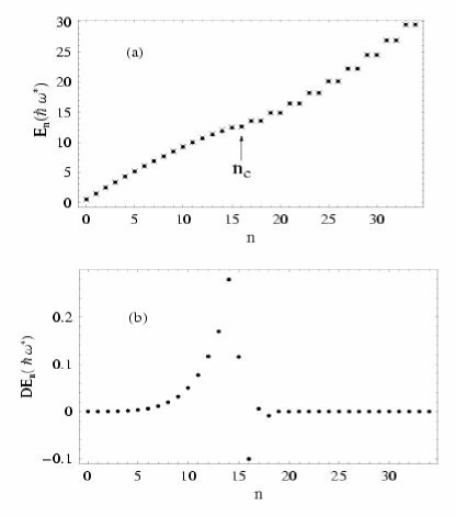
Figure 1: Upper panel (a): Spectrum of a particle in combined quadratic and periodic potentials as a function of the quantum number $n$. The quadratic trap frequency and the depth of the periodic potential are $\omega_{T}=2\pi\times 60$ Hz and $V_{o}=7.4E_{R}$, respectively. Points are numerically obtained values, while crosses are asymptotic expansions of the Mathieu characteristic parameters. The arrow indicates the critical value $n_{c}\approx 2\|\sqrt{q/2}\|$. Lower panel (b): Energy difference $DE_{n}$ between the numerically obtained eigenvalues and the asymptotic expansions.

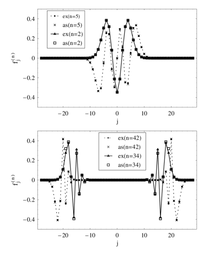
Figure 2: Eigenmodes of a particle in a combined quadratic and periodic potentials as a function of the lattice site $j$. The quadratic trap frequency and the depth of the periodic potential are $\omega_{T}=2\pi\times 60$ Hz and $V_{o}=7.4E_{R}$, respectively. Triangles and dots are numerically obtained values (”ex” in the legend), while boxes and crosses are asymptotic expansions of the Fourier coefficients of the periodic Mathieu functions (”as” in the legend). In the upper panel, triangles and boxes refer to the $n=2$ mode, while dots and crosses refer to $n=5$. In the lower panel, triangles and boxes refer to the $n=34$ mode, while dots and crosses refer to $n=42$.

In Figs. 1 and 2 we compare the above asymptotic approximations to exact numerical results for the eigenenergies and eigenfunctions. The parameters used for the plots are those of a system with a lattice depth of $7.4E_{R}$ and quadratic trap frequency $\omega_{T}=2\pi\times 60$Hz. These values correspond to $J=0.0357E_{R}$, $\Omega=0.0009E_{R}$ and $q=157$. Figure 1, upper panel, shows the lowest 35 eigenenergies as a function of the quantum number $n$. The value $n_{c}$, which is equal to $16$ in this case, is indicated by an arrow. The crosses represent the asymptotic solutions, Eq. (14) and (20), and the dots the numerically obtained eigenvalues. On the scale of the graph there is essentially no appreciable difference between the two solutions for the entire spectrum. The difference between the the numerically obtained energies and the asymptotic expansions is plotted in the lower panel of Fig. 1. In the upper panel of Fig.2, asymptotic expressions for the LE eigenvectors $n=2$(boxes) and $n=5$(crosses) are compared to the numerically obtained eigenmodes (triangles and dots respectively). The modes clearly exhibit an harmonic oscillator character, and the agreement between the asymptotic and numerical solutions is very good. In the lower panel, the $n=34$ and $n=42$ eigenstates belonging to the region $n>n_{c}$ are depicted. These states are localized far from the trap center. While the overall shape of the modes is well reproduced by the asymptotic solutions, for the chosen values of $n$ small differences between the asymptotic (boxes and crosses respectively) and numerical solutions (triangles and dots respectively) can be observed. As expected, the convergence of the asymptotic expansion to the exact solution is better for $n=42$ than for $n=34$, as the former has a larger value of $n$ than the latter.

II.2.2 Low $q$ regime ($4J<\Omega$)

This parameter regime is relevant for deep lattices. When $4J<\Omega$ the kinetic energy required for an atom to hop from one site to the next one is insufficient to overcome the trapping energy even at the trap center and all the modes are localized. This is consistent with the previous analysis, because when $4J\lesssim\Omega$, $n_{c}$ is less than one. The asymptotic expressions that describe this regime are AS64

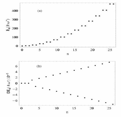
Figure 3: Upper panel (a): Spectrum of a particle in combined quadratic and periodic potentials as a function of the quantum number $n$. The quadratic trap frequency and the depth of the periodic potential are $\omega_{T}=2\pi\times 60$ Hz and $V_{o}=50.0E_{R}$, respectively. Points are numerically obtained values, while crosses are asymptotic expansions of the Mathieu characteristic parameters in the low $q$ limit. Lower panel (b): Energy difference $DE_{n}$ between the numerically obtained eigenvalues and the asymptotic expansions.

$$E^{{\rm{Low}}q}_{n=0}\approx\frac{\Omega}{4}\left(-q^{2}\frac{1}{2}+q^{4}\frac{7}{128}+\dots\right)$$

$$E^{{\rm{Low}}q}_{n=1}\approx\frac{\Omega}{4}\left(4-q^{2}\frac{1}{12}+q^{4}\frac{5}{13824}+\dots\right)$$

$$E^{{\rm{Low}}q}_{n=2}\approx\frac{\Omega}{4}\left(4+q^{2}\frac{5}{12}-q^{4}\frac{763}{13824}+\dots\right)$$

$$E^{{\rm{Low}}q}_{n=3}\approx\frac{\Omega}{4}\left(16+q^{2}\frac{1}{30}-q^{4}\frac{317}{864000}+\dots\right)$$

$$E^{{\rm{Low}}q}_{n=4}\approx\frac{\Omega}{4}\left(16+q^{2}\frac{1}{30}+q^{4}\frac{433}{864000}+\dots\right)$$

$$E^{{\rm{Low}}q}_{n\geqslant 5}\approx E^{high}_{n\geqslant 5}$$ (24)

and

$${{f_{j}}^{{(\rm{Low}})}}^{n=0} \approx A_{0}\left\{\frac{\delta_{j,0}}{\sqrt{8}}+\frac{q}{\sqrt{8}}\delta_{j,1}+\frac{q^{2}}{32}\frac{\delta_{j,2}-\delta_{j,0}}{\sqrt{2}}\right\}$$

$$+\big{\{}j\rightarrow-j\big{\}}$$

$${{f_{j}}^{{(\rm{Low})}}}^{n=1} \approx A_{1}\left\{\delta_{j,1}+\frac{q}{12}\delta_{j,2}+q^{2}\left(\frac{\delta_{j,3}}{384}-\frac{\delta_{j,1}}{288}\right)\right\}$$

$$-\big{\{}j\rightarrow-j\big{\}}$$

$${{f_{j}}^{{(\rm{Low})}}}^{n=2} \approx A_{2}\left\{\delta_{j,1}+\frac{q}{12}\left(\delta_{j,2}-\frac{3}{2}\delta_{j,0}\right)+\right.$$

$$\left.q^{2}\left(\frac{\delta_{j,3}}{384}-19\frac{\delta_{j,1}}{288}\right)\right\}+\big{\{}j\rightarrow-j\big{\}}$$

$${{f_{j}}^{{(\rm{Low})}}}^{n\geq 3} = {f_{j}^{(high)}}^{n\geq 3}$$ (25)

with $A_{n}$ normalization constants. In Fig. 3 the above expansions for the energies are compared with the numerically calculated spectrum. Here the lattice is $50E_{R}$ deep and the external trap frequency is $\omega_{T}=2\pi\times 60Hz$. These lead to values of $J,\Omega$ and $q$ given by $J=2.9\times 10^{-5}E_{R}$, $\Omega=0.0009E_{R}$ and $q=0.13$. The asymptotic and numerical solutions perfectly agree on the scale of the graph. The energy difference between the numerically obtained eigenvalues and the asymptotic expansions is plotted in Fig. 3, lower panel.

III Center of mass evolution of a displaced system

In recent experiments, the transport properties of one dimensional Bose-Einstein condensates loaded in an optical lattice have been studied after a sudden displacement of the quadratic trap trey . A strong dissipative dynamics was observed even for very small displacements and shallow depths of the optical lattice. This should be contrasted with previous experiments performed with weakly interacting 3D gases where very small damping of the center of mass motion was observed for small trap displacements Cataliotti ; Morsch . Recent theoretical studies have demonstrated that the strongly damped oscillations observed in one dimensional systems reflect the importance of quantum fluctuations as the dimensionality is reduced polkovnikov1 ; polkovnikov2 ; polkovnikov3 ; julio .

In this section we study the dipolar motion of ideal bosonic and fermionic gases trapped in the combined lattice and harmonic potentials. We start by writing an expression for the evolution of the center of mass of an ideal gas with general quantum statistics, and then we use this expression to study the dipole oscillations for bosonic and fermionic systems. The simplicity of the noninteracting treatment allows us to derive analytic equations for the dipole dynamics for both statistics.

Later on, in section IV, we show how the knowledge of the bosonic and fermionic ideal gas dynamics can be useful in describing the dynamics of the interacting bosonic system for a large range of parameters of the trapping potentials.

III.1 Ideal gas dynamics

Consider an ideal gas of $N$ atoms loaded in the ground state of an optical lattice plus a quadratic potential initially displaced from the trap center by $\delta$ lattice sites. The initial state of the gas is described by a mixed ensemble state with mean occupation numbers determined by the appropriate quantum statistics

$$z_{j}(t=0) = \frac{1}{N}\sum_{n}\overline{n}_{n}f^{(n)}_{j-\delta},$$ (26)

$$\overline{n}_{n} = \frac{1}{e^{\frac{E_{n}-\mu}{k_{B}T}}\pm 1},$$ (27)

where $T$ is the initial temperature of the system, $k_{B}$ is the Boltzmann constant, $\mu$ is the chemical potential which fixes the total number of particles to $N$, $\sum\overline{n}_{n}=N$, and the positive and negative signs in Eq.(27) are for fermions or bosons, respectively.

The time evolution of the center of mass of the gas is dictated by the ensemble average

$$\langle x(t)\rangle = \frac{1}{N}\sum_{n}\overline{n}_{n}\langle x_{n}(t)\rangle$$ (28)

with

$$\langle x_{n}(t)\rangle = a\sum_{k,l}\left(c_{l}^{(n)}c_{k}^{(n)}e^{-i(E_{k}-E_{l})t/\hbar}\sum_{j}jf_{j}^{(k)}f_{j}^{(l)*}\right)$$

$$c_{k}^{(n)} = \sum_{j}f_{j-\delta}^{(n)}f_{j}^{(k)},$$ (29)

where the quantities $f_{j}^{(n)}$ and the energies $E^{(n)}$ correspond to eigenvalues and eigenenergies of the undisplaced system. The coefficients $c_{k}^{(n)}$ are given by the projection of the $n$ excited displaced eigenstate onto the $k$ excited undisplaced one.

Once the $E_{n}$ and $f^{(n)}_{j}$ are known, the center of mass evolution can be calculated. In the following we discuss the zero temperature dynamics for the ideal bosonic and fermionic systems.

III.1.1 Bosonic system

At zero temperature the bosons are Bose condensed and $\overline{n}_{n}=N\delta_{n0}$, where $\delta_{n0}$ is the Kronecker delta function. The center of mass motion is then given by

$$\langle x(t)\rangle = a\sum_{k,l}\left(c_{l}^{(0)}c_{k}^{(0)}e^{-i(E_{k}-E_{l})t/\hbar}\sum_{j}jf_{j}^{(k)}f_{j}^{(l)*}\right)$$

$$c_{k}^{(0)} = \sum_{j}f_{j-\delta}^{(0)}f_{j}^{(k)}.$$ (30)

If the initial displacement of the atomic cloud is small, $2\delta\ll n_{c}$, and the lattice is not very deep ($q\gg 1$), localized eigenstates are initially not populated. Then, only low-energy states are relevant for the dynamics and the latter can be modeled by utilizing the asymptotic expansions derived in Sec. II.2. To simplify the calculations, we use the harmonic oscillator approximation for the eigenmodes (Eq.(16)), and include up to the quadratic corrections in $n$ in the eigenenergies, which corresponds to keep the first three terms of Eq.(14)). Even though this treatment is not exact, we found that it properly accounts for the period and amplitudes of the center of mass oscillations for small trap displacement. After some algebra it is possible to show that the time evolution of the center of mass is given by

$$\langle x\rangle=a\delta e^{-\left(\frac{\delta^{2}}{a_{ho}^{2}}\sin^{2}\left(\frac{\Omega t}{8\hbar}\right)\right)}\cos\left(\omega_{o}^{*}t-\frac{\delta^{2}}{2a_{ho}^{2}}\sin\left(\frac{\Omega t}{4\hbar}\right)\right)$$ (31)

with $\hbar\omega_{o}^{*}=\hbar\omega^{*}-\Omega/4$.

In Fig. 4 we plot the average center of mass position in units of the lattice spacing $a$ as a function of time for an ideal bosonic system of atoms with ⁸⁷Rb mass. The solid line is obtained by numerically solving the tight binding Schrödinger equation, Eq.(3), while the dotted line is the analytical solution Eq.(31). For the plot we used $V_{o}=7.4E_{R}$, $\omega_{T}=2\pi\times 60Hz$ and $\delta=3$. The time is shown in units of $T_{o}=2\pi/\omega^{*}$, a characteristic time scale. The two solutions exhibit very good agreement for the times shown.

The modulation of the dipole oscillations predicted by Eq.(31) can be observed in the plot. At early times, $t\ll\hbar/\Omega$, the amplitude decreases exponentially as $\exp(-\Gamma_{o}t^{2})$, with $\Gamma_{o}=\left(\frac{\Omega\delta}{8\hbar a_{ho}}\right)^{2}$, and the frequency is shifted from $\omega^{*}$ by $\frac{\Omega}{4\hbar}(1-\frac{\delta^{2}}{2a_{ho}^{2}})$. The initial decay does not correspond to real damping in a dissipative sense, as in a closed system the energy is conserved. The decay is just an initial modulation and after some time revivals must be observed. Because in the large $q$ limit $\omega_{0}^{*}\ll\Omega/\hbar$, the revival time is approximately given by $4h/\Omega$.

It is a general result that the dipole oscillations of a harmonically confined gas in absence of the lattice are undamped. The undamped behavior holds independently of the temperature, quantum statistics and interaction effects (generalized Kohn theorem Kohn ). Equation (31) shows how this result does not apply when the optical lattice is present even for an ideal Bose gas.

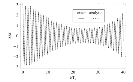
Figure 4: Center of mass motion in lattice units as a function of time for an ideal bosonic gas. In the plot, $V_{o}=7.4E_{R}$, $\omega_{T}=2\pi\times 60Hz$ and $\delta=3$. The time has been rescaled by $T_{o}=2\pi/\omega^{*}$. The solid and dotted lines are the numerical and analytical solution Eq. (31), respectively.

Recent experimental developments have opened the possibility to create a non-interacting gas for any given strength of the trapping potentials feshbach1 ; feshbach2 . The techniques utilize Feshbach resonances for tuning the atomic scattering length to zero. These developments should allow for the experimental observation of the modulation of the dipole oscillations of an ideal gas predicted in this section.

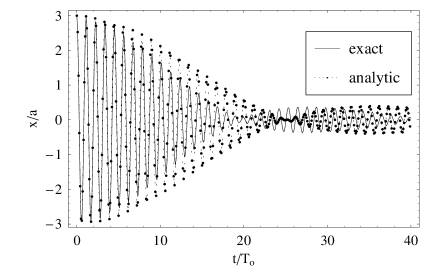
Figure 5: Center of mass motion in lattice units as a function of time for $N=15$ fermions. Here $\omega_{T}=2\pi\times 20Hz$ and $V_{o}=7.4E_{R}$ and $\delta=3$. The time is in units of $T_{o}=2\pi/\omega^{*}$. The solid and dotted lines are the numerical and analytical solution Eq. (34), respectively.

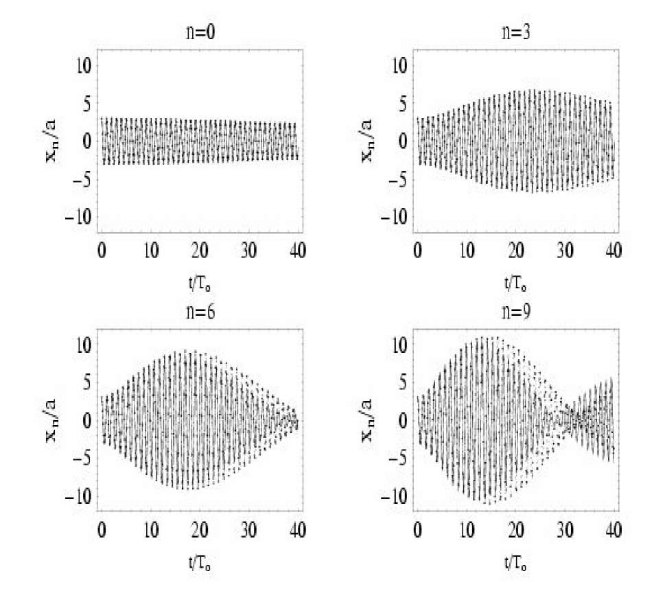
Figure 6: Center of mass motion in lattice units as a function of time for some initially occupied modes. The modes are labeled by the quantum number $n$. As in Fig. 5, the parameters are $\omega_{T}=2\pi\times 20Hz$, $V_{o}=7.4E_{R}$, $N=15$, $\delta=3$ and the time is in units of $T_{o}=2\pi/\omega^{*}$. The solid line corresponds to the numerical solution and the dotted line to the solution given by Eq. (34). When the center of mass evolution of all the different modes is added, from $n=0$ to $n=N-1$ one recovers the total center of mass evolution shown in Fig. 5.

III.1.2 Fermionic system

At zero temperature the Pauli exclusion principle forces fermions to occupy the lowest $N$ eigenmodes, and therefore $\bar{n}_{n}=1$ for $0\leq n\leq N-1$ and zero elsewhere. The occupation of the first $N$ displaced modes makes the condition of occupying only low-energy eigenstates of the undisplaced potentials more restrictive than in the bosonic case. Nevertheless, if the initial displacement, lattice depth and atom number are chosen such that only LE eigenstates are initially populated, $\sum_{n=n_{c}-1}^{\infty}|c_{n}^{(N-1)}|^{2}\ll 1$, it is possible to derive simple analytic expressions for the dipole dynamics. This is the focus of the remainder of this section. Population of localized states considerably complicates the system’s dynamics and a numerical analysis is therefore required. This is postponed to Sec.IV.2.2.

When only LE undisplaced eigenstates are occupied, as explained for the bosonic system, to a good approximation the eigenmodes can be assumed to be the harmonic oscillator eigenstates and only corrections quadratic in the quantum number $n$ are relevant in Eq.(14). After some algebra, the above approximations yield the following expression for the time evolution of the center of mass:

$$\langle x(t)\rangle = \frac{1}{N}\sum_{n=0}^{N-1}\langle x_{n}(t)\rangle$$ (32)

$$\langle x_{n}(t)\rangle \equiv a\delta{\rm{Re}}\left(\exp\left\{i\omega_{o}^{*}t-\left(\frac{\delta^{2}(1-\chi(t))}{2a_{ho}^{2}}\right)\right\}\tilde{x}_{n}(t)\right)$$ (33)

$$\tilde{x}_{n}(t) \equiv \sum_{k=0}^{n-1}\left(\left(\frac{\delta}{a_{ho}}\right)^{2k}\frac{(\chi(t)-1)^{2k}\chi(t)^{n-1-k}((n+1)\chi(t)+k-n)}{(2k)!!(k+1)!}\prod_{s=1}^{k}(n+1-s)\right)+\frac{\left(\frac{\delta}{a_{ho}}\right)^{2n}(1-\chi(t))^{2n}}{(2n)!!}$$ (34)

where $\chi(t)=\exp^{(-i\Omega t/(4\hbar))}$ and $\hbar\omega_{o}*=\hbar\omega^{*}-\Omega/4$.

The parameter $\chi(t)$ takes into account the quadratic corrections to the harmonic oscillator energies. The corrections are proportional to $\Omega/4$, and due to the presence of the lattice. In the limit $\chi(t)\rightarrow 1$, $\tilde{x}_{n}(t)\rightarrow 1$ $\forall n$ and therefore the amplitude of the dipole oscillations remains constant in time, $\langle x\rangle=d\delta\cos(\omega^{*}t)$, as predicted by Kohn theorem. The corrections quadratic in $n$ cause the modulation of center of mass oscillations.

The modulation is caused not only by the overall envelope generated by the exponential term $\exp\left(-\delta^{2}(1-\chi(t))/(2\tilde{a}_{ho}^{2})\right)$, which was also present in the bosonic case, but mainly from the interference created by the different evolution of the $N$ average positions $\langle x_{n}\rangle$ in the sum Eq.(32). The latter induces a fast initial decay of the amplitude of the dipole oscillations.

In Fig.5 we plot the center of mass motion of the fermionic gas composed of $N=15$ atoms with the mass of ⁸⁷Rb. The solid and dotted lines correspond to the numerical and analytic solutions, respectively. Here the depth of the optical lattice is $7.4E_{R}$, and $\omega_{T}=2\pi\times 20Hz$. The amplitude of oscillation shows a rapid decay in time. The analytic solution captures the overall qualitative behavior of the numerical curve. Nevertheless, only at short times the agreement is quantitatively good. Population of eigenstates which are not fully harmonic in character is responsible for the disagreement at later times. This effect is particularly relevant for the evolution of the displaced states with larger quantum number, as explicitly shown in Fig. 6 where the time evolution of some displaced modes is plotted. Again, the solid line is the numerical solution and the dotted line is the analytic one. For the lowest energy modes, $n=0$ and $n=3$, the agreement between the two curves is almost perfect. For the higher energy modes $n=6$ and $n=9$ the analytic solution is underdamped and overestimates the collapse time.

Interestingly, the dynamics of the displaced excited modes exhibits an initial growth of the amplitude. This behavior is a pure quantum mechanical phenomenon due to the constructive interference between the different phases of the undisplaced eigenmodes during the evolution. We explicitly checked for energy conservation during the time evolution. The amplitude increase is captured by the analytic solution and it allowed us to show that the growth happens only when the ratio between the initial displacement $\delta$ and $a_{ho}$ is less than one. While such a behavior is not observable in the evolution of a fermionic cloud, as the observable is the center of mass position summed over all initially populated modes $\langle x(t)\rangle$, the experimental observation of growth for an individual mode may be possible if an ideal bosonic gas is initially loaded in a particular excited state, and then suddenly displaced.

As described above, the evolution of LE modes can be handled analytically. On the other hand, when high-energy eigenmodes are populated the dynamics is much more complicated. Nevertheless, there is another simple limiting case that can be actually solved. This corresponds to the case when the displacement is large enough or the lattice deep enough that the displaced cloud has non-vanishing projection amplitudes only onto high-energy undisplaced modes which can be roughly approximated by position eigenstates, $f_{j}^{2r,2r-1}\approx(\delta_{j,r}\pm\delta_{-j,r})/\sqrt{2}$. Then, one finds that $\langle x_{n}\rangle\approx a\delta$ for all $n$ and thus $\langle x\rangle\approx a\delta$. That is, when only high-energy eigenmodes are populated the dynamics is completely overdamped and the cloud tends to remain frozen at the initial displaced position. We show later on in Sec. IV.2.2 where we treat interacting atoms, that in the so-called Mott insulator regime most populated modes are actually localized, and this kind of overdamped behavior characterizes the dipole dynamics.

IV Many-body system

IV.1 Spectrum of the BH-Hamiltonian in presence of an external quadratic potential

The Bose-Hubbard (BH) Hamiltonian describes the system’s dynamics when the lattice is loaded such that only the lowest vibrational level of each lattice site is occupied Jaksch

$$H_{BH}=\sum_{j}\left[\Omega j^{2}\hat{n}_{j}-J(\hat{a}_{j}^{\dagger}\hat{a}_{j+1}+\hat{a}_{j+1}^{\dagger}\hat{a}_{j})+\frac{U}{2}\hat{n}_{j}(\hat{n}_{j}-1)\right].\\$$ (35)

Here $\hat{a}_{j}$($\hat{a}^{\dagger}_{j}$) is the bosonic annihilation(creation) operator of a particle at site $j$ and $\hat{n}_{j}=\hat{a}_{j}^{\dagger}\hat{a}_{j}$. $\Omega$ and $J$ are defined as in Eqs. (4) and (5), while $U$ is an on-site interaction energy given by $U=\frac{4\pi a_{s}\hbar^{2}}{m}\int dx|w(x_{0})|^{4}$, with $a_{s}$ the s-wave scattering length and $w_{0}(x)$ the first-band Wannier state centered at the origin. The quantity $U$ is the energy cost for having two atoms at the same lattice site. The tunneling rate decreases for sinusoidal lattices with the axial lattice depth $V_{o}$ as

$$J=A\left(\frac{V_{o}}{E_{R}}\right)^{B}\exp\left(-C\sqrt{\frac{V_{o}}{E_{R}}}\right)E_{R},$$ (36)

where the numerically obtained constants are $A=1.397$, $B=1.051$ and $C=2.121$. The interaction energy increases with $V_{o}$ as

$$U=\beta E_{R}\left(\frac{V_{o}}{E_{R}}\right)^{1/4},$$ (37)

where $\beta$ is a dimensionless constant proportional to $a_{s}$. In current experiments, the one-dimensional lattice is obtained by tightly confining in two directions atoms loaded in a three-dimensional lattice. In this case $\beta=4\sqrt{2\pi}(a_{s}/\lambda)(V_{\perp}/E_{R})^{1/2}$, where $V_{\perp}$ is the depth of the lattice in the transverse directions anat ; Olshanii . The parameter $\gamma=U/J$ therefore increases as a function of the axial lattice depth as

$$\gamma(V_{o})=\frac{\beta}{A}\left(\frac{V_{o}}{E_{R}}\right)^{1/4-B}\exp\left(C\sqrt{\frac{V_{o}}{E_{R}}}\right).$$ (38)

In the absence of the external quadratic potential, the bosonic spectrum is fully characterized by the ratio between the interaction and kinetic energies $\gamma$ and the filling factor $N/M$, where $M$ is the number of lattice sites Fisher . For $\gamma\ll 1$ and any $N/M$ ratio the system is weakly interacting and superfluid. For $\gamma\gg 1$ and $M\geq N$ the system fermionizes to minimize the inter-particle repulsion. In this regime the bosonic energy spectrum mimics the fermionic one, the correspondence being exact in the limit of infinitely strong interactions. In particular, in a lattice model the onset of fermionization is characterized by suppression of multiple particle occupancy of single sites. This implies that fermionization occurs for eigenstates whose energy is lower than the interaction energy $U$. If $M>N$ there are $M!/(N!(M-N)!)$ fermionized eigenmodes and the dynamics at energies much lower than $U$ can be accounted for by using these states only. On the other hand, if the lattice is commensurately filled, $N=M$, there is only one fermionized eigenstate, and it corresponds to the ground state. All excited states have at least one multiply occupied site, and therefore excitations are not fermionized. The ground state corresponds to the Mott state with a single particle per site and reduced number fluctuations. The transition from the superfluid to the Mott state is a quantum phase transition, and the critical point for one-dimensional unit filled lattices is $\gamma_{c}\simeq 4.65$ Fisher ; Bat90 .

In the presence of the quadratic trap the spectrum is determined by an interplay of $U$, $J$, $\Omega$ and $N$. In trapped systems the notion of lattice commensurability becomes meaningless because the size of the wave-function is explicitly determined by these parameters. As a consequence, for any value of $N$ the ground state can be made to be a Mott insulator with one atom per site at the trap center by an appropriate choice of $U$, $J$ and $\Omega$ GAG , and the lowest energy modes can always be made to be fermionized in the large $U$ limit. The purpose of this section is to characterize fermionization and localization of the many-body wave-function when both the quadratic and periodic potentials are present, by relating the occurrence of the different regimes to changes in the spectrum at low energies.

We performed exact diagonalizations of the BH-Hamiltonian for $N=5$ particles and $M=19$ sites in presence of a quadratic trap of frequency $\omega_{T}=2\pi\times 150$ Hz. For the calculations, we chose ⁸⁷Rb atoms with scattering length $a_{s}=5.31$ nm, a lattice constant $a=405$ nm, and therefore $\Omega\simeq 0.0046E_{R}$. We fixed the transverse lattice confinement to $V_{\perp}\simeq 25.5$ $E_{r}$ and varied the depth of the optical lattice $V_{o}$ in the parallel direction from 2 $E_{R}$ to about 17 $E_{R}$. For these lattice depths, the energies $U$ and $J$ both vary so that their ratio $\gamma$ increases from $3.3$ to about $150$. Due to the changes in $J$, the ratio $q=4J/\Omega$ characterizing the single-particle solutions decreases from 130 to 4 with increasing $V_{o}$. The effective harmonic-oscillator energy spacing $\hbar\omega^{*}$ decreases approximately from 0.0525 $E_{R}$ to 0.0092 $E_{R}$. We used these parameters because they are experimentally feasible and fulfill the condition $U-\Omega((N-1)/2)^{2}>0$ for the entire range of the trapping potentials. Later on we discuss that, for deep enough lattices, fulfillment of the last inequality ensures the existence of an energy range in which eigenmodes are fermionized.

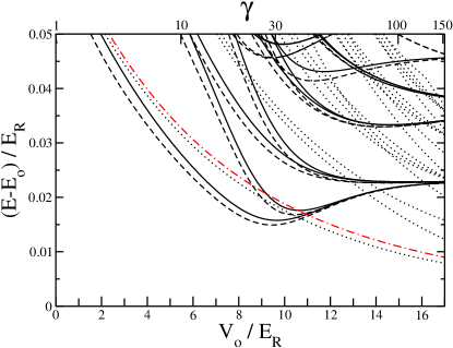
Figure 7: Energy spectra as a function of the depth of the axial optical lattice $V_{o}$. The continuous, dotted and dashed lines correspond to $N=5$ interacting bosons, non-interacting bosons and fermions, respectively. The dashed-dotted line corresponds to $\hbar\omega^{*}$. The horizontal axis on the top of the figure is $\gamma=U/J$, and is only meaningful for interacting bosons. For each energy spectrum, the corresponding ground-state energy $E_{0}$ has been subtracted.

Figure 7 shows the lowest eigenergies of the BH-Hamiltonian as a function of $V_{o}$. The continuous line is the exact solution for $N=5$ interacting bosons. The dotted and dashed lines are the exact spectra for 5 non-interacting bosons and fermions, respectively. They have the same mass and are trapped in the same potentials as the interacting bosons. Their spectra are shown for comparison purposes. For each spectrum the energy $E_{0}$ of the ground state has been subtracted.

In the absence of the optical lattice, $V_{o}=0$, the energy difference $\Delta E_{0}=E_{1}-E_{0}$, or energy spacing, between the first excited and ground state equals the harmonic oscillator level spacing $\hbar\omega_{T}$, independent of statistics and interaction strength. Figure 7 show that this is no longer the case in the presence of the lattice.

The dependence of $\Delta E_{0}$ on statistics is evident in the plot, as the level spacing is different for ideal bosons and fermions. In particular, the energy spacing for bosons is only shifted from $\hbar\omega^{*}=\sqrt{4\Omega J}$ (dashed-dotted line) by an amount which is almost constant for all lattice depths, while $\Delta E_{0}$ for fermions clearly deviates from $\hbar\omega^{*}$, especially for deep lattices. The behavior of $\Delta E_{0}$ in the two cases can be understood by using the asymptotic solutions of the single-particle problem. For ideal bosons $\Delta E_{0}$ is equal to the energy difference between the first-excited and ground single-particle eigenenergies. The ratio $q$ used for the plots is such that the critical value $n_{c}$ of Eq. (23) is always larger than 2, and therefore the ground and first-excited eigenenergies are well described by Eq. (14). The calculation of the energy difference using this equation yields $\Delta E_{0}\approx\hbar\omega^{*}-\Omega/4$. For fermions, $\Delta E_{0}$ is equal to the difference between the energies of the $n=N$ and $n=N-1$ single-particle excited states. For $V_{o}<9.6E_{R}$, the critical value $n_{c}$ is larger than $N$, and therefore the energies of the $n=N$ and $n=N-1$ single-particle excited states are also well described by Eq. (14). Then, $\Delta E_{0}$ for fermions is smaller than for bosons because lattice corrections are more important for higher quantum numbers, and have all negative sign. On the other hand, for $V_{o}>9.6E_{R}$, $n_{c}$ is smaller than $N-1$ and the energies of the $n=N$ and $n=N-1$ single-particle excited states are described by Eq. (20). The transition of the single-particle eigenmodes at the Fermi level from LE to HE around $V_{0}=9.6E_{R}$ is signaled by the minimum of $\Delta E_{0}$ for fermions. In general, an estimate for the value of $J$ at which the minimum takes place is

$$J\sim\Omega((N-1)/2)^{2}/2.$$ (39)

This value is obtained by equating the Fermi energy $E_{N-1}$, which is of order $\Omega((N-1)/2)^{2}$ from Eq. (20), to $E_{n_{c}}$, which is approximately $2J$. The transition of the single-particle eigenmode at the Fermi level from LE to HE is also connected to the formation of a region of particle localization at the trap center in the many-body density profile. As explained in Rigol , when $E_{N-1}$ is equal to $E_{n_{c}}$ the on-site density in the central site of the trap approaches 1 with reduced fluctuations. For $V_{0}>9.6E_{R}$, Fig. 7 shows that $\Delta E_{0}$ approaches an asymptotic value $\Omega N$, value that can be derived from Eq. (20). When the asymptotic value $\Omega N$ is reached, most single-particle states below the Fermi level are localized, and this yields a many-body density profile with $N$ unit-filled lattice sites at the trap center.

The dependence of the first excitation energy on interactions can also be seen in Fig. 7. In fact, by comparing $\Delta E_{0}$ for the interacting bosons to the value of $\Delta E_{0}$ for ideal bosons and fermions, three different regimes can be considered: $1\lesssim\gamma\lesssim 10$, $10\lesssim\gamma\lesssim 30$ and $\gamma>30$. These regimes correspond to the intermediate, fermionized-non-localized and fermionized-Mott regimes, respectively. The weakly interacting regime $\gamma\lesssim 1$ is only reached for $V_{o}\ll 2E_{R}$ for our choice of atoms and trapping potentials. For such lattice depths the tight-binding approximation is not valid, and therefore we do not show the spectra for this regime in Fig. 7. In the following we discuss the main features of the different regimes focusing on the connection to the ideal bosonic and fermionic systems.

$\bullet$ For $\gamma\leq 1$ the interacting bosonic system is in the weakly interacting regime. In this regime the first excitation energy is almost the same as the ideal bosonic one. Most atoms are Bose-condensed, interaction-induced correlations can be treated as a small perturbation, and the spectrum can be shown to be well reproduced by utilizing Bogoliubov theory anabog .

$\bullet$ For $1<\gamma<10$, the system is in the intermediate regime, where $\Delta E_{0}$ for interacting bosons deviates from the ideal bosonic energy spacing and approaches the ideal fermionic one. Indeed, Fig.7 shows that for $V_{0}\lesssim 4E_{R}$, $\Delta E_{0}$ for the interacting bosons lies closer to the ideal bosonic energy spacing, while for $V_{0}>4$ it lies closer to the ideal fermionic one. In the presence of the optical lattice $\gamma$ increases exponentially with $V_{o}$, and therefore the intermediate regime occurs for a relatively small range of accessible trapping potentials, here for $1\lesssim V_{o}/E_{R}\lesssim 5.5$.

$\bullet$ For $\gamma\geq 10$ the interacting spectrum approaches the ideal Fermi spectrum and the system is in the fermionized regime. The numerical solutions show that the energy difference between the energy spectra of interacting bosons and fermions is of the order of $J^{2}/U$ and slightly increases for larger frequencies of the quadratic trap.

In general, fermionization in the presence of the external quadratic potential occurs for $N<M$ when the two following inequalities are satisfied

$$\gamma=U/J\gg 1,U>\Omega((N-1)/2)^{2}.$$ (40)

While the first inequality is the same as for homogeneous lattices and relates to the building of particle correlations, the second inequality is specific to the trapped case and relates to suppression of double particle occupancy of single sites. If the interaction energy $U$ is larger than the largest trapping energy, which corresponds to trapping an atom at position $(N-1)/2$, it is energetically favorable to have at most one atom per well. The average on-site occupation is therefore less or equal to one.

The second inequality in Eq. (40) poses some limitations on the choice of possible $\Omega$ and $U$ for a given number of trapped particles. For our choice of the trapping potentials, this inequality is satisfied for any $V_{o}$. Indeed, this is not an unrealistic assumption. In recent experiments with ⁸⁷Rb atoms, an array of fermionized gases has been created with at most 18 atoms per tube Paredes . For such $N$, the condition $U>\Omega((N-1)/2)^{2}$ can be fulfilled for many different choices of experimentally feasible trapping potentials.

Figure 8: Density profiles $n_{j}\equiv\langle\hat{n}_{j}\rangle$ as a function of the lattice site $j$ for different lattice depths. The dash-dotted, dashed and dotted lines correspond to interacting bosons, while the boxes, dots and triangles correspond to ideal fermions for $V_{o}/E_{R}=7,12$ and $15$ lattice depths, respectively.

Figure 9: Number fluctuations $\Delta n_{j}\equiv\sqrt{\langle\hat{n}_{j}^{2}\rangle-\langle\hat{n}_{j}\rangle^{2}}$ as a function of the lattice site $j$ for different lattice depths. Conventions and parameters are the same as in Fig.8

$\bullet$ For $\gamma>30$ the system enters the fermionized-Mott regime. In fact, Fig. 7 shows that for $\gamma>30$ the energy spacing for the interacting bosons (and also for ideal fermions) begins to increase until it reaches an asymptotic value at $\gamma\approx 150$.

The approaching of the asymptotic value signals the formation of a localized many-body state for the interacting bosons, the so-called Mott insulator state. The relevant relation between $N$, $\Omega$ and $J$ for the formation of an extended core of unit-filled sites at the trap center with fluctuations mainly at the outermost occupied sites is

$$\Omega N\geq J.$$ (41)

This is explained as $\Omega N$ is the energy cost for moving a particle from position $|(N-1)/2|$ to position $|(N+1)/2|$ at the borders of the occupied lattice and it is the lowest excitation energy deep in the Mott state.

Figure 7 shows that for $\gamma\approx 150$ the energies of the first four excited states become degenerate. This degeneracy occurs because deep in the Mott regime the energy required to shift all the atoms of one lattice site to the right or left is the same as the energy required for moving an atom from site $\pm(N-1)/2$ to site $\pm(N+1)/2$. For $\gamma\approx 150$, $J$ is approximately $\Omega$, and therefore the tunneling energy is barely sufficient to overcome the potential energy cost $\Omega$ for moving a particle from the central site of the trap to one of its neighbors. In the single-particle picture,when $J\approx\Omega$ all the single-particle states below $E_{N-1}$ are localized.

In order to better understand the formation of the Mott insulator, in Figs. 8 and 9 the on-site particle number $n_{j}=\langle\hat{n}_{j}\rangle$ and fluctuations $\Delta n_{j}=\sqrt{\langle\hat{n}_{j}^{2}\rangle-\langle\hat{n}_{j}\rangle^{2}}$ are plotted as a function of the lattice site $j$, for different lattice depths $V_{o}$. The lines and symbols are the results for interacting bosons and ideal fermions, respectively. All the $V_{o}$-values are such that the interacting bosonic system is fermionized. This is mirrored by the overall good agreement between lines and symbols for all the curves. The plots show that for $V_{o}=7E_{R}(\gamma=15$, dashed-dotted line), the largest average particle occupation is $n_{0}\approx 0.7$, and number fluctuations are of the order of $0.5$ in the central 9 sites, while for $V_{o}=12E_{R}(\gamma=54$, dashed line), $n_{0}$ approaches 1 in the central 3 sites, and fluctuations at the trap center drop to a value $\Delta n_{j}\approx 0.1$. The sharp drop in particle fluctuations clearly signals the localization at the trap center, and is in agreement with $J<\Omega N$ for $\gamma=54$. For $V_{o}=15E_{R}(\gamma=104$, dotted line), the Mott state is formed, as the mean particle number in the five central sites is one, with nearly no fluctuations. Fluctuations are larger at lattice sites far from the center, and due to the tunneling of particles to unoccupied sites.
Because of the small number of atoms that we use in the calculations, $\Omega((N-1)/2)^{2}/2$ and $\Omega N$ are of the same order of magnitude. It is therefore not possible to clearly distinguish the value of $J$ for which the on-site density at the trap center approaches one from the value of $J$ for which the Mott state is fully formed at the trap center, with reduced number fluctuations in the central $N$ sites. Preliminary results obtained with a Quantum Monte-Carlo code, Worm Algorithm Proko , confirm the existence of these two distinct parameter regions when more atoms are considered, and therefore the usefulness of both the energy scales $\Omega((N-1)/2)^{2}/2$ and $\Omega N$ for interacting bosons. These results will be published elsewhere.

IV.2 Many-body dynamics

In this section we study the temporal dipole dynamics of an interacting bosonic system composed of 5 atoms trapped in a combined quadratic plus periodic confinement. The role of interactions on the effective damping of the dipole oscillations is studied by means of exact diagonalization of the Hamiltonian. As discussed when dealing with the ideal gas dynamics, such damping is effective because it is due to dephasing and does not have a dissipative character.

Assuming the system is initially at $T=0$, the evolution of the center of mass is given by:

$$\langle x(t)\rangle = \sum_{l,k}A_{lk}e^{i\omega_{lk}t}$$ (42)

$$A_{lk} \equiv a\sum_{j}j\langle\phi_{l}|\hat{n}_{j}|\phi_{k}\rangle C_{l}^{*}C_{k},$$ (43)

with $\hbar\omega_{lk}\equiv E_{l}-E_{k}$ and where $E_{l}$ and $|\phi_{l}\rangle$ are eigenvalues and eigenmodes of the BH-Hamiltonian. The coefficients $C_{l}$ are the projections of the initial displaced ground state $|\varphi(0)\rangle$ onto the eigenfunctions $\{|\phi\rangle_{l}\}$ of the undisplaced Hamiltonian, $C_{l}=\langle\phi_{l}|\varphi(0)\rangle$.

For the exact evolution, the ground-state $|\varphi(0)\rangle$ is calculated by shifting the center of the quadratic trap by $\delta$ lattice sites. The number of wells $M$ is 19 for all simulations, which fixes the size of the Hilbert space to 33649. In the time propagation we only keep those eigenstates whose coefficients $C_{l}$ are such that $|C_{l}|^{2}>10^{-3}$. The typical number of states that fulfil this requirement is about 100. The accuracy of the truncation of the Hilbert space during the time propagation has been checked by increasing the number of retained states, finding no appreciable changes in the dynamics.

We are interested in the dynamics both when a Mott insulator state is not and is present at the trap center. These two cases are discussed in Secs.IV.2.1 and IV.2.2, respectively. In particular, in Sec. IV.2.1 the interaction strength $U$ is varied, while the ratio $q$, specifying the ideal gas dynamics, is large and constant. For the chosen values of $q$ and $N$, $J>\Omega N$ and for increasing $U$ the system fermionizes without forming a Mott insulator at the trap center. In Sec. IV.2.2, the dynamics of systems that do exhibit a Mott insulator in the large $U$ limit is analyzed. In this case, $J$ and $U$ are simultaneously varied by increasing the axial optical lattice depth.

IV.2.1 Non-localized dynamics

In the absence of the optical lattice, the equations of motion for the center of mass are decoupled from those of the relative coordinates. As only the latter are affected by interactions, all modes excited during the collective oscillations have the harmonic oscillator energy spacing $\hbar\omega_{T}$, and therefore $\langle x(t)\rangle=\langle x(0)\rangle\cos(\omega_{T}t)$.

When the lattice is present, the equations of motion for the center of mass and relative coordinates are coupled, and thus the many-body dynamics is interaction dependent. In this section we fix $\omega_{T}=2\pi\times 100Hz$ and $V_{o}=7E_{R}$, and study the role of interactions in the many-atom dynamics by varying $\gamma$ from $0$ to $200$, for constant $q=77$. This can be experimentally realized by tuning the scattering length of the system by means of Feshbach resonances. In the following, we analyze the weakly interacting, intermediate and strongly interacting regimes separately.

Weakly interacting regime: $\gamma\leq 1$

In order to study the role of interactions in the weakly interacting regime, in Fig. 10 the effective damping constant of dipole oscillations $\Gamma$ is shown as a function of $\gamma$. The damping constant was calculated by fitting the first 10 center of mass oscillations to the ansatz $\langle x(t)\rangle=a\delta\exp{(-\Gamma t^{2})}\cos(\omega t)$, where $\Gamma$ and $\omega$ are fitting parameters. This ansatz is chosen in analogy to the non-interacting model. The effective damping $\Gamma$ is in units of $\Gamma_{o}=\delta^{2}\Omega^{2}/(8\hbar a_{ho})^{2}$, which is the damping constant predicted by Eq. 31. The solid and dotted lines correspond to $\Gamma$ as calculated by means of exact diagonalizations and by numerically evolving the following Discrete Non-Linear Schrödinger Equation (DNLSE) for the amplitudes $\{z_{j}\}$

$$i\hbar\frac{\partial z_{j}}{\partial t}=-J(z_{j+1}+z_{j-1})+\Omega j^{2}z_{j}+U|z_{j}|^{2}z_{j},$$ (44)

respectively. Eq.(44) has been obtained by replacing the field operator $\hat{a}_{j}$ with the c-number $z_{j}(t)$ in the Heisenberg equation of motion for $\hat{a}_{j}$. Such replacement is justified for $\gamma\ll 1$ as the many-body state is almost a product over identical single-particle wave-functions. The amplitudes $\{z_{j}\}$ satisfy the normalization condition $\sum_{j}|z_{j}|^{2}=N$. The initial state used in the evolution of the DNLSE was found by numerically solving for the ground state of Eq. (44), displaced by $\delta=2$ lattice sites.

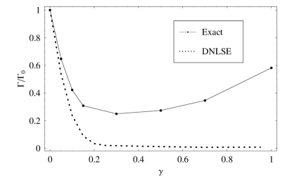
Figure 10: Effective damping constant of the dipole oscillations as a function of $\gamma$ for a system in the weakly interacting regime. Here, $q\approx 77$, $\omega_{T}=100$ Hz and $\Gamma_{o}=\left(\delta\Omega/8\hbar a_{ho}\right)^{2}$.

In Fig. 10, the continuous and dotted lines overlap for $\gamma\leq 0.05$, and show a decrease in the damping constant with increasing interaction strength in the whole range $\gamma\leq 0.2$. For values of $\gamma>0.05$ the mean field and exact solutions start to disagree. While the exact solution has a minimum around $\gamma\approx 0.2$, and then grows for larger $\gamma$ values, the mean field curve decreases monotonically to zero.

The fact that the mean-field solution decreases to zero for increasing interactions is explained by noting that when interaction effects become important the density profile acquires the form of an inverted parabola, or Thomas-Fermi profile, $|z_{j}^{TF}(t)|^{2}\approx\Omega\left((j-\langle x(0)\rangle/a)^{2}-R_{\rm{TF}}^{2}\right)/U$, $\langle x(0)\rangle=a\delta$. Substitution of the Thomas-Fermi profile in Eq. (44) leads to the exact cancellation of the quadratic potential, and thus, in the frame co-moving with the atomic cloud, the atoms feel an effective linear potential. The spectrum of a linear plus periodic potential is known to be equally spaced Stark , and therefore no damping due to dephasing is expected.

It is important to note that the mean-field undamped oscillation occurs only in a parameter regime far from dynamical instabilities. In fact, as shown in previous theoretical and experimental studies wu ; Burger ; smerzi , when the initial displacement is large enough to populate states above half of the lattice band-width, mean-field dynamical instabilities induce a chaotic dipole dynamics. In the framework of this paper, this critical displacement corresponds to $\delta\approx n_{c}/2$. For $\delta>n_{c}/2$, the initial ground-state has a significant overlap with localized eigenmodes of the undisplaced system, which are therefore populated during the dipolar dynamics, causing damping. The importance of the population of these modes is enhanced by the non-linear term, which causes an abrupt suppression of the center of mass oscillations at the critical point in the mean-field solution.

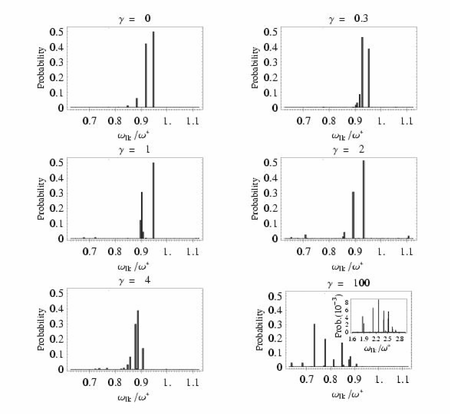
Figure 11: Probability distribution of frequencies for different values of $\gamma$, with $q\approx 77$ and $\omega_{T}=100$ Hz. The frequencies $\omega_{lk}$ are in units of $\omega^{*}$.

While the mean-field anaysis accounts for the decrease in the damping constant, Fig. 10 shows that it is not accurate for $\gamma\gtrsim 0.2$. This is due to the fact that the mean-field analysis completely neglects interaction-induced correlations. These correlations are responsible for the quantum depletion of the condensate, which causes some atoms to be excited to higher-energy single-particle eigenmodes which are more affected by the lattice. To show this effect in a quantitative manner, in Fig.11 we plot the probability distribution of the frequencies $\omega_{lk}$, Eq. (42), for some values of $\gamma$. In the histograms, the height of a bar-chart centered at a given frequency $\omega$ is the occurrence probability of $\omega_{lk}$. The probability is proportional to the normalized sum over all the weight factors $|A_{lk}|$ whose frequency lies between $\omega_{lk}-0.0025$ and $\omega_{lk}+0.0025$. The frequencies are in units of the effective harmonic oscillator frequency $\omega^{*}$ of Eq. (17). This approach is similar to the one used in Ref. Lundh , where the strength function is used to study the collective dynamics induced by mono- and dipolar excitations.

The histogram for the case $\gamma=0$ shows a frequency distribution with most frequencies in the interval $0.85\omega^{*}\leq\omega_{lk}\leq 0.96\omega^{*}$. In particular, two large peaks are observed in the range $0.9\omega^{*}\leq\omega_{lk}\leq 0.96\omega^{*}$. This is to be compared to the case where the lattice is not present, and a single peak at $\omega^{*}$ is expected. The observed frequency spread is due to the modification of the harmonic oscillator spectrum introduced by the lattice and is responsible for the observed damping in the ideal bosonic gas, as explained in detail in Sec. III.1.1.

Figure 11 also shows that for $\gamma=0.3$ the system has a narrower frequency distribution. In this case approximately $100\%$ of the frequencies lie in the interval $0.9\omega^{*}\leq\omega_{lk}\leq 0.96\omega^{*}$. The frequency narrowing from $\gamma=0$ to $\gamma=0.3$ is consistent with the decrease in the damping constant shown in Fig. 10. For larger values of $\gamma$, $\gamma=1$ and $2$, some modes with frequency smaller than $0.7\omega^{*}$ and larger than $1.1\omega^{*}$ start to contribute to the collective dynamics. Population of such modes is related to the depletion of the condensate and signal the increased importance of quantum fluctuations in the system.

Finally, we note that for our choice of $\Omega$, $N$ and $J$, $\Omega((N-1)/2)^{2}/J$ is approximately $0.2$, which is the value of $\gamma=U/J$ at which the mean-field and exact solutions begin to disagree. This suggests that the fulfillment of the second inequality in Eq. (40), $U>\Omega((N-1)/2)^{2}$, is related to the failure of the mean-field approach, even for $\gamma<1$.

Intermediate Regime: $1<\gamma<10$

Figure 12: Effective damping rate of the dipole oscillations $\Gamma$ as a function of $\gamma$ in the intermediate and strongly correlated regimes. Here, $q\approx 77$ and $\omega_{T}=100$ Hz. The damping rate has been rescaled such that $\Gamma(\gamma=1)=1$. The large and small dots are for interacting bosons and non-interacting fermions, respectively. The continuous line is a guide for the eye. The dashed line is the best-fit curve $\Gamma=10.13\exp(-16.4\gamma^{-1.25})$ to the exact damping rate for interacting bosons.

In Fig. 12 the numerically obtained damping constant is shown for $\gamma>1$. In this parameter regime we find that the function $a\delta\exp(-\Gamma t^{2})\cos(\omega t)$ does not provide a good fit to the center of mass evolution. Instead, we find that a better fitting ansatz is given by $a\delta\exp(-\Gamma t)\cos(\omega t)$ . In the plot, the damping constant is normalized to $\Gamma_{1}$, which is the damping rate at $\gamma=1$.

We observe that for $2\leq\gamma<5$ the damping is almost constant. This is consistent with the fact that by inspection the spectrum of excited frequencies has a similar shape and width in the entire transition region. An example of such a frequency distribution is given in Fig. 11 for $\gamma=4$. The dominant peak is around $\omega_{lk}\approx 0.9\omega^{*}$, while multiple peaks are noticeable between $0.7\omega^{*}\leq\omega_{lk}\leq 0.92\omega^{*}$. The overall envelope of the distribution has a long tail, as opposed to the case $\gamma=1$ where all the weight is roughly concentrated in just two frequencies.

The increased importance of the tails of the distribution for $\gamma>1$ qualitatively accounts for the transition from an exponential decay quadratic in time towards an exponential decay which is linear in time. In fact, for $\gamma<1$ the probability distribution of frequencies may be fitted by a Gaussian, while for $\gamma>1$ a better fit is provided by a Lorentzian-like profile. The Fourier transforms of such distributions give precisely the observed functional form of the decay of the dipole oscillations.

Strongly interacting regime $\gamma>10$

In Fig. 12 for $\gamma>10$, the damping rate is shown to rapidly increase and approach a finite asymptotic value which is depicted in the plot by a dotted line. This asymptotic value $\Gamma_{\infty}$ corresponds to the damping rate calculated for an ideal fermionic gas. The fermionic damping rate is constant because here $J$ and $\Omega$ are kept constant while $U$ increases. The tendency to approach the fermionic damping rate as $\gamma$ increases is a consequence of fermionization of the bosonic wave-functions for $\gamma\gg 1$, Eq. (40). Numerically we find that the damping rate approaches $\Gamma_{\infty}$ exponentially, $\Gamma(\gamma)=\Gamma_{\infty}\exp(-a\gamma^{\alpha})$, with a best-fit exponent $\alpha$ of order $-1$. The fitting curve is shown in the plot with a dashed line.

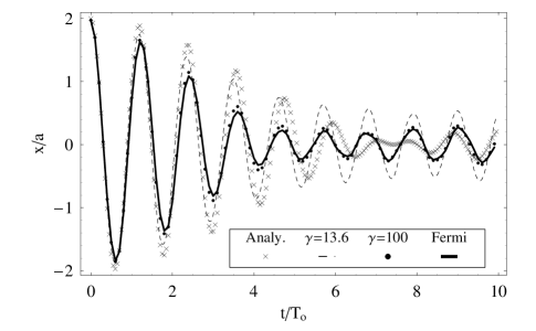
Figure 13: Center of mass position in lattice units as a function of time for interacting bosons, for $\gamma=13.6$(dashed line) and $\gamma=100$(dots). The solid line is the center of mass position for ideal fermions, while the crosses are the analytical approximation to the fermionic solution Eq.(34). Here, $q\approx 77$ and $\omega_{T}=2\pi\times 100$ Hz and $T_{o}=2\pi/\omega^{*}$.

The dipole dynamics of the bosonic and fermionic systems are explicitly compared in Fig. 13, where we plot the first 10 oscillations of the center of mass after the sudden displacement of the trap. In the figure, the dashed line and the dots are the bosonic dynamics for $\gamma=13.6$ and 100, the solid line is the fermionic evolution, and the crosses are the analytical approximation to the fermionic evolution Eq. (34), respectively. Consistent with Fig. 12, we observe that for increasing $\gamma$ the decrease of the amplitude of oscillation for the bosons resembles more and more the one for fermions. In particular, for $\gamma=100$, the curves for the interacting bosons and ideal fermions nearly overlap. The distribution of excited frequencies for $\gamma=100$ is shown in Fig. 11. The frequency distribution is broad and centered around $\omega\approx 0.75\omega^{*}$. Also in the inset small peaks are shown to appear in the range $1.6\omega^{*}\leq\omega\leq 3\omega^{*}$ (notice the different scale in the inset). The broad distribution is due to the population of single-particle states that are not harmonic in character. For the value of $q$ used for the calculations no single-particle localized modes are occupied in the ground state before the trap displacement. After the displacement about 90 percent of the atoms occupy non localized single-particle modes. The phase mixing between these modes accounts for most of the observed damping. The remaining 10 percent occupy localized states and the population of these modes is responsible for the shift of the peak of the distribution to lower frequency. In fact we show below, Sec. IV.2.2, that a large population of localized states with $n\gg n_{c}$ yields a distribution which is peaked at $\omega\approx 0$.

Finally, we note that the small population of localized modes after the displacement also explains why the analytic solution Eq.(34) reproduces the exact fermionic evolution in Fig. 13 only qualitatively. In fact, Eq.(34) was derived under the condition $\sum_{n=n_{c}-1}|c_{n}^{(N-1)}|^{2}\ll 1$, while here $n_{c}=12$ and $\sum_{n=11}|c_{n}^{(N-1)}|^{2}\approx 0.1$.

IV.2.2 Localized dynamics

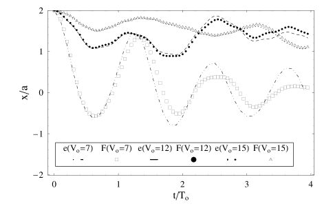
Figure 14: Center of mass position (in lattice sites) as a function of time calculated for different lattice depths and a fixed $\omega_{T}=2\pi\times 150$ Hz. The dash-dotted, dashed and small-dotted lines are the exact solutions for interacting bosons (e in the legend) and the boxes, large-dots and triangles are the solutions for ideal fermions (F in the legend ) for $V_{o}/E_{R}=7,12$ and $15$, respectively. $T_{o}=2\pi/\omega^{*}$.

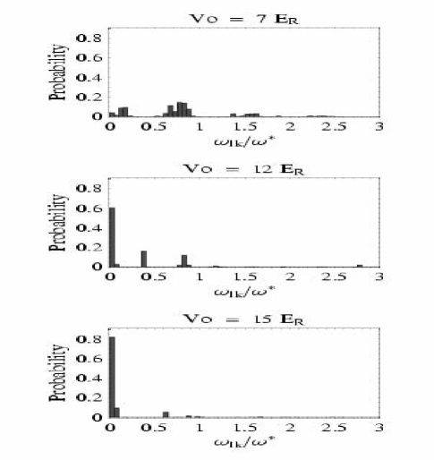
Figure 15: Probability distribution of frequencies for $V_{o}/E_{R}=7,12$ and $15$ (see text). The frequencies $\omega_{lk}$ are given in units of $\omega^{*}$. Because $\omega^{*}\propto\sqrt{J}$, $\omega^{*}$ decreases with increasing lattice depth.

In analogy to recent experiments trey , in this section we study the dipole dynamics when the depth $V_{o}$ of the optical lattice is varied, while the parabolic confinement is kept constant. Then, both $J$ and $U$ change as a function of the lattice depth, as explained in Sec. IV. The parabolic confinement $\omega_{T}=2\pi\times 150Hz$ has been chosen to be the same as in Sec. IV, so that the energy spectrum exactly matches the one discussed there, when $V_{o}$ is varied.

In Fig.  14 lines and symbols correspond to the time evolution of the interacting bosons and ideal fermions, respectively. In particular, the dashed-dotted, dashed and small-dotted lines are for bosons, while boxes, large-dots and triangles are for fermions with $V_{o}/E_{R}=7,12$ and $15$, respectively. For such lattice depths $\gamma=14,50$ and 100, respectively, and the system is fermionized, as discussed in Sec. IV.1. As expected, the agreement between the bosonic and fermionic solutions improves for larger $\gamma$-values, and is almost perfect for $\gamma=100$.

Notably, for all the $\gamma$-values, no complete oscillation are observed, as the amplitudes of oscillations are strongly damped at very early times. The inhibition of the transport properties in the experiment here envisioned is a direct consequence of the large population of single-particle states which are localized in character. For the case $V_{o}=7E_{R}$ ($\Omega N/J\approx 0.58$, $\gamma=13.6$ , $q=134.2$ and $n_{c}\approx 8$) before the displacement the system is fermionized but non-localized. On the other hand, after the displacement about 20 percent of the atoms occupy localized modes of the undisplaced potential. The population of the localized modes with $n\gg n_{c}$ can be directly linked to the presence of low-frequency peaks ($\omega_{lk}\approx 0$) in the distribution of frequencies, Fig. 15. Because 80 percent of the atoms occupy non-localized modes the center of mass position can still relax to zero as shown in Fig.14. For the cases $V_{o}=12E_{R}$ and $15E_{R}$ the Fermi energy is larger than $E_{n_{c}}$, and even before the displacement most states are localized. After the displacement has taken place, about 60 and 90 percent of the atoms occupy localized modes respectively, and the dynamics is overdamped. This is mirrored by the appearance of a large peak at $\omega_{lk}\approx 0$ in the probability distribution, Fig.15, and by the fact that the center of mass position does not relax to zero as shown in Fig.14.

V Conclusions

We studied the spectrum and dipolar motion of interacting and non-interacting one-dimensional atomic gases trapped in an optical lattice plus a parabolic potential using the tight-binding approximation. We showed that the single-atom tight-binding Schrödinger equation can be exactly solved by mapping it onto the recurrence relation satisfied by the Fourier coefficients of some periodic Mathieu functions. We used asymptotic expansions of such functions to fully characterize the eigenenergies and eigenmodes of the system. Our analytic approach is complementary to previous numerical and semiclassical analysis for single-atom systems. The advantage is that we could explicitly calculate the corrections to the harmonic oscillator spectrum introduced by the lattice. The knowledge of these corrections allowed us also to provide analytic expressions for the modulations of the center of mass motion induced by the periodic potential when trapped ideal bosonic and fermionic gases are suddenly displaced from the trap center.

By means of numerical diagonalizations of the Bose-Hubbard Hamiltonian we studied the interacting many-body bosonic problem. First, we characterized the changes in the low-energy excitation spectrum as a function of lattice depth, by comparing it with the ideal Bose and Fermi spectra. Then, we stated the necessary conditions for fermionization to occur and showed that it takes place for a large range of experimentally accessible parameters. We clarified the required conditions for the formation of a Mott insulator at the trap center and linked its appearance to the population of localized states at the Fermi level of the correspondent ideal fermionic system. We then studied the many-body dipole dynamics and showed that, in the parameter regime where the system is expected to be fermionized, the knowledge of the single-particle solutions is a powerful tool for the understanding of the strongly correlated dynamics. By studying the distribution of the frequencies pertaining the many-body modes excited during the dipole dynamics, we explicitly showed the connection between the population of single-particle localized states with the inhibition of the transport properties of the system. These spectral analysis allowed us also to gain some insight into the dynamics in the weakly-interacting regime, where an analysis beyond mean-field is required, and in the complex intermediate regime, where no mapping to single-particle solution is possible.

VI Acknowledgement

We thank Trey Porto and Eite Tiesinga for useful discussions. We acknowledge financial support from an the Advanced Research and Development Activity (ARDA) contract and the U.S. National Science Foundation under grant PHY-0100767.

Note: We note that some of the points discussed here have been just recently pointed out in Ref.Rigol3 where the authors discuss the dipole oscillations of 1D bosons in the hard-core limit.

References

- (1) B. Laburthe Tolra, K. M. O’Hara, J. H. Huckans, W. D. Phillips, S. L. Rolston, and J.V. Porto, Phys. Rev. Lett. 92, 190401 (2004).
- (2) H. Moritz, T. Stöferle, M. Köhl, and T. Esslinger, Phys. Rev. Lett. 91, 250402 (2003).
- (3) T. Stöferle, H. Moritz, C. Schori, M. Köhl, T. Esslinger, Phys.Rev. Lett. 92, 130403 (2004).
- (4) B. Paredes, A. Widera, V. Murg, O. Mandel, S. Fölling, I. Cirac, G. V. Shlyapnikov, T. W. Hänsch, and I. Bloch, Nature 429, 277 (2004).
- (5) T. Kinoshita, T. Wenger and D. S. Weiss, Science 305, 1125 (2004).
- (6) M. Girardeau, J. Math. Phys. 1, 516 (1960).
- (7) E. H. Lieb and W. Liniger, Phys. Rev. 130, 1605 (1963).
- (8) L. Pezzè, L. Pitaevskii, A. Smerzi, S. Stringari, G. Modugno, E. de Mirandes, F. Ferlaino, H. Ott, G. Roati, and M. Inguscio, Phys. Rev. Lett. 93, 120401 (2004).
- (9) H. Ott, E. de Mirandes, F. Ferlaino, G. Roati, V. Türck, G. Modugno, and M. Inguscio, Phys. Rev. Lett. 93, 120407 (2004).
- (10) V. Ruuska and P. Törmä, New J. of Phys. 6,59 (2004).
- (11) Anatoli Polkovnikov, Subir Sachdev, and S. M. Girvin, Phys. Rev. A 66, 053607 (2002).
- (12) C. Hooley and J. Quintanilla, Phys. Rev. Lett. 93, 080404 (2004).
- (13) M. Rigol and A. Muramatsu, Phys. Rev. A 70, 043627 (2004).
- (14) I. Abramowitz and I. A. Stegun, Handbook of Mathematical Functions, National Bureau of Standards (1964).
- (15) J. Meixner and F.W. Schäfke, Mathieusche funktionen und sph roidfunktionen, Springer-Verlag (1954); N.W. McLachlan, Theory and Application of Mathieu Functions, Dover (1964).
- (16) M. Aunola , J. Math. Phys. 44, 1913 (2003).
- (17) N. W. Ashcroft and N. D. Mermin, Solid State Physics, W. B. Saunders Company (1976).
- (18) J. M. Ziman, Principles of the Theory of Solids, Cambridge University Press (1964).
- (19) C. D. Fertig, K. M. O’Hara, J. H. Huckans, S. L. Rolston, W. D. Phillips, and J. V. Porto, cond-mat/0410491 (2004).
- (20) O. Morsch, J. H. Müller, M. Cristiani, D. Ciampini, and E. Arimondo, Phys. Rev. Lett. 87, 140402 (2001).
- (21) F. S. Cataliotti, S. Burger, C. Fort, P. Maddaloni, F. Minardi, A. Trombettoni, A. Smerzi, and M. Inguscio, Science 293, 843 (2001).
- (22) A. Polkovnikov and D.-W.Wang, Phys. Rev. Lett. 93, 070401 (2004).
- (23) A. Polkovnikov, E. Altman, E. Demler, B. Halperin and M.D. Lukin, cond-mat/0412497 (2004).
- (24) E. Altman, A. Polkovnikov, E. Demler, B. Halperin, and M. D. Lukin, cond-mat/0411047 (2004).
- (25) J. Gea-Banacloche, A. M. Rey, G. Pupillo, C.J. Williams, and C.W. Clark, cond-mat/0410677 (2004).
- (26) W. Kohn, Phys. Rev. 123, 1242 (1961); J. F. Dobson, Phys. Rev. Lett. 73, 2244 (1994).
- (27) S. L. Cornish, N. R. Claussen, J. L. Roberts, E. A. Cornell, and C. E. Wieman, Phys. Rev. Lett. 85, 1795 (2000).
- (28) E. A. Donley, N. R. Claussen, S. L. Cornish, J. L. Roberts, E. A. Cornell, and C. E. Wieman, Nature 412, 295 (2001).
- (29) D. Jaksch,C. Bruder, J. I. Cirac, C. W. Gardiner and P. Zoller, Phys. Rev. Lett. 81, 3108 (1998).
- (30) A.M. Rey, Ultra cold bosonic atoms in optical lattices, D. Phil. Thesis, Maryland University at College Park ( 2004).
- (31) M. Olshanii and V. Dunjko, Phys. Rev. Lett. 91, 090401 (2003).
- (32) M. P. A. Fisher, P. B. M. Weichman, G. Grinstein and D.S. Fisher, Phys. Rev. B 40, 546 (1989).
- (33) G. G. Batrouni, R. T. Scalettar, and G. T. Zimanyi, Phys. Rev. Lett. 65, 1765 (1990).
- (34) G. Pupillo, A.M. Rey, G.K. Brennen, C.J. Williams, and C.W. Clark, J. of Mod. Opt. 51, 2395 (2004).
- (35) A.M. Rey ,K. Burnett ,R. Roth , M. Edwards , C.J. Williams, C.W.Clark , J. Phys. B: At. Mol. Opt. Phys, 36 , 825 (2003).
- (36) H. Fukuyama, R.A. Bari, and H.C. Fogedby, Phys. Rev. B 8, 5579 (1973); G. Wannier, Phys. Rev. 17, 432 (1960).
- (37) B. Wu, R. B. Diener, and Q. Niu, Phys. Rev. A 65, 025601 (2002), and references therein.
- (38) S. Burger, F. S. Cataliotti, C. Fort, F. Minardi, M. Inguscio, M. L. Chiofalo, and M. P. Tosi, Phys. Rev. Lett. 86, 4447 (2001).
- (39) A. Smerzi, A. Trombettoni, P. G. Kevrekidis, and A. R. Bishop, Phys. Rev. Lett. 89, 170402 (2002).
- (40) M. Greiner, O. Mandel, T. Esslinger,T. W. Hänsch, and I. Bloch, Nature 415, 39 (2002).
- (41) N. V. Prokof’ev, B. V. Svistunov, and I. S. Tupitsyn, Phys. Lett. A 238, 253 (1998); JETP 87, 310 (1998).
- (42) E. Lundh, Phys. Rev. A 70, 061602 (2004).
- (43) M. Rigol, V. Rousseau, R. T. Scalettar and R. R. P. Singh, cond-mat/0503302.