A quantum Monte Carlo study on the superconducting Kosterlitz-Thouless transition of the attractive Hubbard model on a triangular lattice

Abstract

We study the superconducting Kosterlitz-Thouless transition of the attractive Hubbard model on a two-dimensional triangular lattice using auxiliary field quantum Monte Carlo method for system sizes up to $12\times 12$ sites. Combining three methods to analyze the numerical data, we find, for the attractive interaction of $U=-4t$, that the transition temperature stays almost constant within the band filling range of $1.0<n<1.4$, while it is found to be much lower in the $n<1$ region.

I Introduction

Discovery of superconductivity in layered materials or quasi-two-dimensional systems in the past several decades has brought up great interest in the physics of low dimensional superconductors. Among those are the high $T_{c}$ cuprates,BM a ruthenate Sr₂RuO₄,Maeno a cobaltate Na_xCoO${}_{2}\cdot y$ H₂O,Takada MgB₂,Akimitsu a heavy electron system CeCoIn₅,Petrovic and organic conductors such as (BEDT-TTF)₂X (X is an anion).McKenzie

Theoretically, it is well known by Mermin-Wagner’s theorem that no off-diagonal long range order takes place at finite temperature in purely two-dimensional(2D) systems.MW In the case of pure 2D, superconducting transition is expected to be of the Kosterlitz-Thouless (KT) type.KT The superconducting KT transition has previously been studied using finite temperature auxiliary field quantum Monte Carlo (AFQMC) technique for the attractive Hubbard model, that is, the Hubbard model with a negative on-site $U$, on a square latticeMS and on a triangular lattice.Santos Nowadays, a renewed interest for the KT transition on triangular lattices has arisen because unconventional superconductivity has been observed in materials having (anisotropic) triangular lattice structure such as Na_xCoO${}_{2}\cdot y$H₂O and (BEDT-TTF)₂X.

For the square lattice, it has been shown that the KT superconducting transition temperature $T_{0}\sim 0.1t$, $t$ is the hopping integral, for square lattice with $n=0.87$ ($n$ is the band filling) away from the half filling $n=1.0$, where charge density wave (CDW) ordering takes place.MS As for the triangular lattice, it has been concluded that $T_{0}$ takes its maximum at around half-filling due to the absence of CDW ordering, while $T_{0}$ is low near $n=1.4$,where the density of states becomes large due to the van Hove singularity at $n=1.5$.

Since previous studies have been restricted to small system sizes, here we revisit the problem of the superconducting KT transition of the attractive Hubbard model on a triangular lattice using AFQMC technique. Combining three methods of analyzing the numerical data, we find that the KT transition temperature stays almost constant within the band filling region of $1<n<1.4$.Our results suggest that the estimation of the KT transition temperature using finite size scaling requires some caution when the density of states near the Fermi level is small and the calculation is restricted to small system sizes.

II Formulation

II.1 Model

The Hamiltonian of the attractive Hubbard model is given in standard notation as

$${\cal H} = -t\sum_{\left<i,j\right>,\sigma}(c_{i,\sigma}^{\dagger}c_{j,\sigma}+c_{j,\sigma}^{\dagger}c_{i,\sigma})$$ (1)

$$+U\sum_{i}n_{i,\uparrow}n_{i,\downarrow}-\mu\sum_{i,\sigma}n_{i,\sigma},$$

where $c_{i,\sigma}^{\dagger}(c_{i,\sigma})$ is a fermion creation (annihilation) operator at site $i$ with spin $\sigma$, and $n_{i,\sigma}=c_{i,\sigma}^{\dagger}c_{i,\sigma}$,$<i,j>$ denotes a pair of nearest neighbors on square or triangular lattice having periodic boundary condition.The chemical potential $\mu$ controls the band filling $n$ (average number of electrons per site). The hopping parameter $t$ is taken as the unit of the energy and is set equal to unity throughout the study. As for the lattice structure, we mainly concentrate on the triangular lattice, but we also perform calculation on the square lattice at the band filling of $n=0.87$ in order to make comparison with previous studies and with the triangular lattice. The on-site attraction $U$ is fixed at $U/t=-4.0$ on both lattices, which also enables us to make comparison with the previous studies.

II.2 Pairing Correlation Function

Above the superconducting KT transition temperature $T_{0}$, the on-site ($s$-wave) pairing correlation function decays exponentially,

$$<c_{i,\uparrow}^{\dagger}c_{i,\downarrow}^{\dagger}c_{j,\uparrow}c_{j,\downarrow}>\sim\exp(-r/\xi).$$ (2)

By contrast, the pairing correlation function exhibits a power-law decay

$$<c_{i,\uparrow}^{\dagger}c_{i,\downarrow}^{\dagger}c_{j,\downarrow}c_{j,\uparrow}>\sim r^{-\eta},$$ (3)

where $\eta=0.25$ for $T\rightarrow T_{0}$. In the actual AFQMC calculation, we calculate a summation of the pairing correlation function, $P_{s}$, given as

$$P_{s} = \left<\Delta^{\dagger}\Delta+\Delta\Delta^{\dagger}\right>$$ (4)

$$\Delta^{\dagger} = \frac{1}{\sqrt{N}}\sum_{i}c_{i,\uparrow}^{\dagger}c_{i,\downarrow}^{\dagger}$$ (5)

Due to the decaying behavior of the pairing correlation function mentioned above, $P_{s}$ increases as $N$ is increased below $T_{0}$, while it remains constant above $T_{0}$.

In the present study, finite temperature AFQMC is used to calculate $P_{s}$. Hirsch ; White The number of Trotter decomposition slices $L$ is chosen to satisfy the condition $L\geq 12\beta$ ($\beta=1/T$), so that $\Delta\tau\leq 0.084/t$ is satisfied, where $\Delta\tau=\beta/L$. $3000-30000$ Monte Carlo sweeps, depending on the temperature and system size, have been taken to assure sufficiently small statistical errors. We have performed calculation on system sizes from $4^{2}$ to $12^{2}$ sites.

In order to obtain $T_{0}$ from the AFQMC data of $P_{s}$, we use three methods, two of which are based on finite size scaling, while the other one is a more straightforward method.

II.3 Finite size scaling

As shown in eq.3, the pairing correlation decays as $r^{-\eta}$ below $T_{0}$ for a large system size. Hence $P_{s}$ is proportional to ${N_{x}}^{2-\eta}$ with system size $N=N_{x}^{2}$. In a finite size system,scaling variable $N_{x}/\xi$ ,where $\xi$ is the correlation length, becomes more important.Taking this into account,the scaling hypothesis assumes the following behavior for $P_{s}$.

$$P_{s}(T,N_{x})=N_{x}^{2-\eta}f(N_{x}/\xi)$$ (6)

$$\xi=\exp(A/(T-T_{0})^{1/2}),$$ (7)

where $A$ is a constant and $f(x)$ is a certain scaling function. Since $\xi\rightarrow\infty$ for $T\rightarrow T_{0}$, $f(x)=f(0)$ regardless of the system size $N$ at $T=T_{0}$. Thus, if we plot $P_{s}N_{x}^{-2+\eta}$ as functions of $T$(or $\beta$) for different system sizes, they should coincide regardless of the system size at $T=T_{0}$. Santos

Another method to identify $T_{0}$ is to plot $P_{s}N_{x}^{-2+\eta}$ as a function of $N_{x}/\xi$, where $T_{0}$ and $A$ are chosen so that all the data points fall on a single curve (namely $P_{s}N_{x}^{-2+\eta}=f(N_{x}/\xi)$) regardless of the system size.MS

However, as we shall see in the following, these scaling methods eq.6 turns out to suffer from finite size effects when the system size is small and/or the density of states at the Fermi level is small. In fact, in the former method mentioned above, $P_{s}$ for small system sizes do not coincide with those for large system sizes even at $T=T_{0}$. As for the latter method, $P_{s}N_{x}^{-2+\eta}$ for small system sizes deviate from those for larger system sizes at low temperatures.

Due to this problem, here we identify $T_{0}$ as the temperature at which $P_{s}$ for the largest two system sizes coincide in the former method, while in the latter method, we search the values for $T_{0}$ and $A$ so that as many data points as possible fall on a single curve, although the data for small system sizes deviate from the curve at low temperatures.

II.4 Extrapolation method

Since the scaling method suffers from finite size effects on some cases, we have adopted the third method, namely the extrapolation method. This method has been adopted for the study of the (real) superconducting transition temperature for the three dimensional attractive Hubbard model.Sewer Since $P_{s}$ should increase sharply at $T=T_{0}$ in the thermodynamic limit, it is reasonable to assume that $T_{0}=\lim_{N\rightarrow\infty}T_{1}^{(N)}$, where $T_{1}^{(N)}$ is the inflection point of $P_{s}(T)$ for the $N$ site system. $T_{1}^{(N)}$ can be obtained by fitting $P_{s}(T)$ by an appropriate function. In this study we use a gaussian form $A_{N}\exp[-B_{N}(T-C_{N})^{2}]+D_{N}$ as a fitting function, where $A_{N}$-$D_{N}$ are fitting parameters. Here, we find that $T_{1}^{(N)}$ scales as $1/N$ in the range of $N$ considered in the present study. We may then obtain $T_{0}$ by plotting $T_{1}^{(N)}$ as a function of $1/N$ and linearly extrapolating it to the $1/N\rightarrow 0$ limit.

III Results

III.1 Finite size scaling

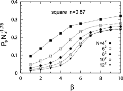
Figure 1: $P_{s}N_{x}^{-1.75}$ plotted against $\beta$ for the square lattice. Dashed lines are guides to the eyes.

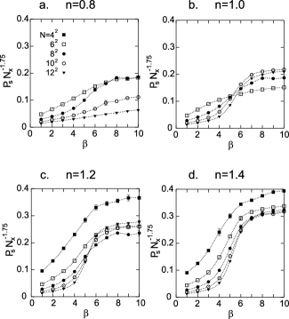
Figure 2: A plot similar to Fig.1 but for triangular lattice with several band filling. Band filling $n$ is $0.8$(a),$1.0$(b),$1.2$(c),$1.4$(d).

We first present finite size scaling analysis, where we identify the temperature at which $P_{s}N_{x}^{-1.75}$ coincides between different system sizes. Before going into the results for the triangular lattice, we show the result for the square lattice with $n=0.87$, where a scaling analysis has been performed for system sizes up to $8\times 8$ in ref.MS, . In Fig.1, $P_{s}N_{x}^{-1.75}$ is plotted as functions of $\beta$ for system sizes from $4\times 4$ to $12\times 12$. We can see that the results for the largest two system sizes, $10\times 10$ and $12\times 12$ merges at around $\beta=7$. The results for smaller systems do not cross or merge with each other within the present temperature range, but if we assume that the results for small systems are strongly affected by finite size effects, we may adopt $T_{0}/t\simeq 1/7\simeq 0.13$ for this band filling, which is roughly consistent with what has been concluded $(T_{0}/t\simeq 0.1)$ in ref.MS, .

We now move on to the results for the triangular lattice. In Fig.2, $P_{s}N_{x}^{-1.75}$ is plotted as functions of $\beta$. For $n=1.4$, the results for the largest two systems, $10\times 10$ and $12\times 12$ merges at around $\beta=6$. The results for smaller systems do not cross or merge with each other within the present temperature range as in the case of the square lattice, but if we again assume that the results for small systems are strongly affected by finite size effects, we may adopt $T_{0}/t\simeq 1/6=0.17$ for this band filling. For $n=1.2$, the results for the largest three system sizes cross at $\beta\simeq 5.3$. Again assuming that results for smaller system sizes are affected by finite size effects, we may take $T_{0}/t\simeq 0.19$ for this band filling. As for $n=1.0$, although the results for $12\times 12$ and $8\times 8$ crosses at around $\beta=6$, those of the largest two sizes do not cross with each other. Therefore, $T_{0}/t$ cannot be estimated from these results at this band filling. The situation is even worse in the case of $n=0.8$, where $P_{s}N_{x}^{-1.75}$ of the largest two system sizes do not even come close at low temperatures. Here again we cannot evaluate $T_{0}/t$ for this band filling from these results.

III.2 Extrapolation method

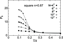
Figure 3: The AFQMC data of pairing correlation function $P_{s}$ for square lattice with $n=0.87$. Dashed curves are the fitting results.

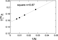
Figure 4: $T_{1}^{N}$ plotted against $1/N$ for the square lattice with $n=0.87$. The dashed line is a least squares fit.

We now evaluate $T_{0}$ using an alternative method, that is, the extrapolation method. Here again, we first show the result for the square lattice with $n=0.87$. In Fig.3, the raw $P_{s}$ data is plotted as functions of temperature for each system size. $T_{1}^{(N)}$ extracted from these data are plotted against $1/N$ in Fig.4. The results for $N=4^{2}$ turn out to be too much affected by finite size effects, so we have omitted these data in the extrapolating process. $T_{0}$ obtained by extrapolating the results to $1/N\rightarrow 0$ is $T_{0}/t\simeq 0.15$, which is a little bit higher than, but in fair agreement with the value obtained by the scaling method.

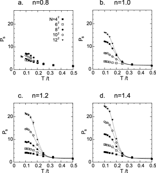
Figure 5: A plot similar to Fig.3 but for the triangular lattice with $n=0.8$(a), $1.0$(b), $1.2$(c), $1.4$(d). Dashed lines are fitting results.

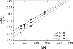
Figure 6: A plot similar to Fig.4 but for the triangular lattice with $n=1.0$, $1.2$, $1.4$.

We move on to the triangular lattice. In Fig.5, the raw $P_{s}$ data as well as the fitting curves are plotted as functions of $T$ for each system size and band filling. (We do not show the fitting curves for $n=0.8$ since $T_{1}^{(N)}$ turns out to be negative.) $T_{1}^{(N)}$ obtained fromthese data are plotted against $1/N$ for each band filling in Fig.6. $T_{0}$ obtained by extrapolation is $0.17$, $0.18$, $0.17$ for $n=1.4$, $n=1.2$, $n=1.0$, respectively. For $n=1.4$ and $n=1.2$, $T_{0}$ obtained using the scaling method coincides fairly well with the values obtained here. For $n=0.8$, $P_{s}$ turns out to decrease upon increasing the system size from $8\times 8$ to $12\times 12$, which seems to indicate that there is no symptom of KT transition within the temperature range $(>0.1t)$ investigated in the present study, so $T_{0}$, if any, should be lower than $0.1t$. In Fig.7, $T_{0}$ obtained by the present method is plotted against the band filling.

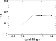
Figure 7: The band filling dependence of the KT transition temperature $T_{0}$. Solid and dashed lines are guides to the eyes.

III.3 Justification by scaling

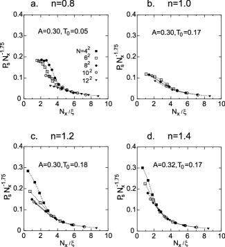
Figure 8: $P_{s}N_{x}^{-1.75}$ plotted against $N_{x}/\xi$ for the triangular lattice.

The KT transition temperature determined by the above method can be further justified by checking whether $P_{s}$ actually scales as $P_{s}=N_{x}^{1.75}f(N_{x}/\xi)$ with $\xi=\exp(A/(T-T_{0})^{1/2}))$. In Fig.8, we plot $P_{s}N_{x}^{-1.75}$ as functions of $N_{x}/\xi$ for all the system sizes. We find for $n=1.0$, $1.2$, and $1.4$ that the numerical results for $8\times 8$, $10\times 10$ and $12\times 12$ fall on a single curve by adopting the $T_{0}$ obtained above and choosing appropriate values of $A$. The results for smaller systems also fall on the same curves at high temperatures (namely for large $N_{x}/\xi$), but at low temperatures they start to deviate due to finite size effects. As for $n=0.8$, if $A=0.3$ and $T_{0}=0.05$ are chosen, the results for $12\times 12$ and $10\times 10$ fall on a similar curve. These results further justify the values of $T_{0}$ obtained in the preceding sections. Similar results are also obtained for the square lattice as seen in Fig.9.

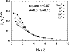
Figure 9: A plot similar to Fig.8 for the square lattice with $n=0.87$.

IV Discussion

IV.1 Comparison of the methods for determining $T_{0}$

Our results show that the scaling method using the crossing point of $P_{s}N_{x}^{-1.75}$ is strongly affected by finite size effects, and that it is difficult to know from the beginning the system size necessary to obtain an accurate $T_{0}$. The present analysis suggests that this method seems to work well at band fillings where the density of states at $E_{F}$ is relatively large, namely at $n=1.2$ and $n=1.4$ in the present case. There, the agreement with the results of the extrapolation method is also good. This may be because the discreteness of the energy levels due to the finite system size is small when the density of states is large.

IV.2 Correlation between $T_{0}$ and the density of states

In order to look into a possible correlation between $T_{0}$ and the density of states at the Fermi level, we compare the present results of $T_{0}$ with the transition temperature obtained by mean field approximation (Fig.11). Although the values of $T_{c}^{\rm MF}$ themselves are much larger than $T_{0}$, we find a similar band filling dependence, namely, $T_{c}^{\rm MF}$ is almost constant for $1<n<1.5$, and smaller for $n<1$. The origin of this similarity is not clear, but this does seem to suggest that $T_{0}$ is roughly correlated with the density of states near the Fermi level at least for the value of $U(=-4t)$ adopted in the present study. It would be an interesting future study to analyze this point from the viewpoint of the study by Timm et al, where the relation between the mean field $T_{c}$ and the KT superconducting transition temperature in the repulsive Hubbard model has been investigated by calculating the superfluid density as a function of temperature and combining it with the Berezinskii-Kosterlitz-Thouless theory.Timm

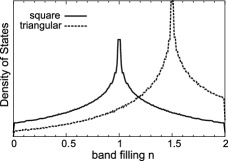
Figure 10: The density of states of the square and the triangular lattices on the tight binding model.

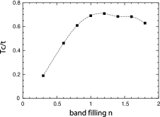
Figure 11: The band filling dependence of the $T_{c}^{MF}$ for the triangular lattice obtained by applying BCS mean field approximation.

$T_{0}$ for $1\leq n\leq 1.4$ is still larger than $T_{0}$ for the square lattice at $n=0.87$ despite the fact that the density of states near the Fermi level for the square lattice with $n=0.87$ is larger than for the triangular lattice with $n=1.0$ (see Fig.10).

If $T_{0}$ is indeed positively correlated with the density of states near the Fermi level, this “inversion” of $T_{0}$ between the square and the triangular lattice may be due to the absence of charge density wave ordering in the latter lattice due to frustration, as discussed previously.Santos

V Conclusions

In the present study, we have investigated the superconducting KT transition of the attractive Hubbard model on a two-dimensional triangular lattice using auxiliary field quantum Monte Carlo method for system sizes up to $12\times 12$ sites. Combining three methods to analyze the numerical data for the pairing correlation function, we find that the transition temperature stays almost constant within the band filling range of $1.0\leq n\leq 1.4$, while it is found to be much lower in the $n<1$ region. Among the three methods, the extrapolation method is found to work well regardless of the band filling, while the methods relying on finite size scaling require some caution when the density of states near the Fermi level is small and the calculation is restricted to small system sizes.

VI Acknowledgements

We thank Yoichi Yanase for valuable discussions. Part of the numerical calculations has been done at the Computer Center, ISSP, University of Tokyo.

References

- (1) J.G. Bednorz and K.A. Müller, Z. Phys. B 64, 189 (1986).
- (2) Y. Maeno, H. Hashimoto, K. Yoshida, S. Nishizaki, T. Fujita, J.G. Bednorz, and F. Lichtenberg, Nature 372, 532 (1994).
- (3) K. Takada, H. Sakurai, E. Takayama-Muromachi, F. Izumi, R. A. Dilanina, and T. Sasaki, Nature 422, 53 (2003).
- (4) J. Nagamatsu, N. Nakagawa, T. Muranaka , Y. Zenitani, and J. Akimitsu, Nature 410, 63 (2001).
- (5) C. Petrovic, P.G. Pagliuso, M.F. Hundley, R. Movshovich, J.L. Sarrao, J.D. Thompson, Z. Fisk, and P. Monthoux, J. Phys.:Condens.Matter 13, L337 (2001).
- (6) For a review, see e.g. R.H. McKenzie, Comments Cond. Matt. Phys. 18, 309 (1998).
- (7) N.D. Mermin and H. Wagner, Phys. Rev. Lett 17, 1133 (1966).
- (8) J.M. Kosterlitz and D.J Thouless, J. Phys. C 6, 1181 (1973).
- (9) A. Moreo and D.J. Scalapino, Phys. Rev. Lett 66, 946 (1991).
- (10) Raimundo R. dos Santos, Phys. Rev. B 48, 3976 (1993).
- (11) S.R. White, D.J. Scalapino, R.L. Sugar, E.Y. Loh, J.E. Gubernatis, and R.T. Scalettar, Phys. Rev. B 40,506 (1989).
- (12) J. E. Hirsch, Phys. Rev. B 31, 4403 (1985).
- (13) A. Sewer, X. Zotos, and Hans Beck, Phys. Rev. B 66,140504(R) (2002).
- (14) C. Timm, D. Manske, and K. H. Bennemann, Phys. Rev. B 66,094515 (2002).