Log-Poisson Statistics and Extended Self-Similarity in Driven Dissipative Systems

Abstract

The Bak-Chen-Tang forest fire model BCT was proposed as a toy model of turbulent systems, where energy (in the form of trees) is injected uniformly and globally, but is dissipated (burns) locally. We review our previous results on the model CB ; BC and present our new results on the statistics of the higher-order moments for the spatial distribution of fires. We show numerically that the spatial distribution of dissipation can be described by Log-Poisson statistics which leads to extended self-similarity (ESS) Benzi93 ; Dubrulle . Similar behavior is also found in models based on directed percolation; this suggests that the concept of Log-Poisson statistics of (appropriately normalized) variables can be used to describe scaling not only in turbulence but also in a wide range of driven dissipative systems.

url]http://www.cz3.nus.edu.sg/$\sim$chenk and

1 Introduction

Understanding the spatial distribution of energy dissipation is crucial in the study of homogenous, isotropic, fluid turbulence. Kolmogorov, in his celebrated 1941 theory (K41) K41 , first conjectured that, in the inertial range, the velocity structure functions scale as a power law in the separation $l$. The theory implicitly assumes uniform energy dissipation characterized by a mean dissipation rate. Experiments from the recent decades showed clear deviations from the K41 scaling, which are believed to be related to the highly intermittent and non-uniform spatial distribution of dissipation. frisch ; sreeni Many phenomenological models of energy cascade and intermittency have been proposed to understand the deviations from the K41 scaling. The most famous are the Lognormal model K62 , the Multifractal model Parisi , and the Log-Poisson model by She and Lévêque (SL) She . The SL model, based on a hypothesis about the behavior of the moments of the energy dissipation, leads to a prediction of the exponents for the velocity structure functions that appears to be in excellent agreement with experimental results. Benzi et al. Benzi93 discovered an important property they termed Extended Self-Similarity (ESS): the $p^{th}$ order structure function has a power-law dependence on the third-order structure function. They found that the validity of ESS extended almost down to the dissipative range, roughly five times the Kolmogorov scale. The connection between the dissipation distribution and the scaling in the inertial range is further supported by these investigations.

It remains a great challenge to understand the dynamical mechanism for the inertial range scaling and ESS in turbulence. So far it has not been feasible to attack the problem directly from the underlying equations for turbulence. Instead we choose to study a few simple models of “turbulent systems”, such as the BCT forest fire model. We hope that, by illustrating the emergence of complex spatial distribution of dissipation and ESS in such simple dynamical models, we can gain some intuition about the dynamical mechanism for energy cascade and scaling in fully developed turbulence.

2 Scale-Dependent Dimension in the BCT Forest Fire Model

The BCT forest fire model is defined as follows. On a $d$-dimensional lattice of size $L^{d}$, trees, representing energy, are grown randomly at empty sites at a rate $p$. At each time step, trees that are on fire are burnt down (the site becomes empty at the next time step) and neighboring trees are ignited. The fires die out when there are no more trees in their neighborhood. These processes represent the dynamics of energy input and dissipation. Numerical studies indicate that there is a correlation length $\xi$ ($\xi\sim p^{-2/3}$ in 3D) in the system CB . If $L\leq\xi$ the fires cannot be sustained, so we consider only the case $L>\xi$. Larger and larger systems can be studied in the limit $p\rightarrow 0$. Despite the simplicity of the model, many fascinating scaling behaviors emerge. For example, Bröker and Grassberger grass found anomalous scaling in three and four dimensions; in particular, they found periodic oscillations in autocorrelation functions with a period $T$ which diverges as $1/p^{\beta}$ with $\beta\,\approx\,0.77$ in three dimensions.

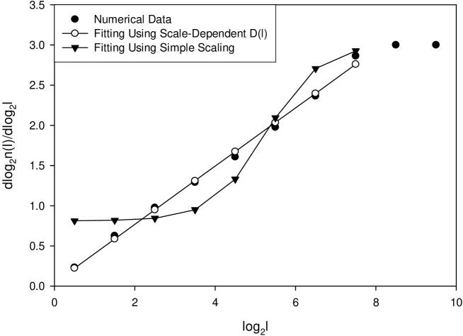
Figure 1: $D(l)$ vs $\log_{2}l$ for the BCT forest fire model with $L=1024$ and $p=0.0003$. Averages were obtained using $10^{6}$ time steps (after skipping $200,000$ time steps). The fits using the expression of scale-dependent dimension and the simple “fractal” scaling with crossover to 3D are also shown.

One of the interesting features of the model is the unconventional scaling that can be interpreted geometrically as a scale-dependent fractal dimension: the apparent dimension $D(l)$ characterizing the distribution of fires at the length scale $l$ in three spatial dimensions increases linearly in $\log(l)$ CB ; BC . The dimension increases gradually as one steps further and further backwards, and views the system at larger and larger length scales. At some point, the correlation length is reached; the distribution of fires remains uniform beyond that length. This is the main geometrical picture for the spatial distribution of the fires. We have repeated the simulation for larger lattices (up to $2048^{3}$) and smaller $p$ (as small as $0.00015$); so far no deviation from the scaling described above is found. As was done in the previous simulation CB , we determine the mean number of fires $n(l)$ within boxes of size $l<\xi$ that contain fires. The linear dependence of $D(l)$ on $\log(l)$ corresponds to

$$\log(n(l))\sim\alpha\frac{\log(l/l_{0})}{\log(\xi/l_{0})}\log(l/l_{0}),$$ (1)

which gives rise to

$$D(l)\equiv\frac{d\log(n(l))}{d\log(l))}=2\alpha\frac{\log(l/l_{0})}{\log(\xi/l_{0})}\,.$$ (2)

Fig. 1 shows the numerical values of $D(l)$ vs $\log_{2}l$. Here $D(l)$ is calculated using the numerical derivative: $D(2^{1/2}l)=\log_{2}(n(2l))-\log_{2}(n(l))$. In the figure we also show the two-parameter fit using the above equation. There is excellent agreement between the data and the our proposed expression of $D(l)$ (even a one-parameter fitting with $l_{0}$ fixed to $l_{0}=1$ is very good). For comparison we also show the fitting using a simple “fractal” scaling: $n(l)=al^{b}+cl^{3}$ which gives $D(l)=(abl^{b}+3cl^{3})/(al^{b}+cl^{3})$. This three-parameter fitting is very bad. It is interesting to note that the distribution of luminous matter in the universe might also follow a scaling form similar to the one given in Eq. 2 BC .

3 Extended Self-Similarity in the Forest Fire Model

The scale dependent dimension shown in the previous section only concerns the first moment of the fire distribution. We will show that the higher-order moments also exhibit interesting scaling behaviors. Preliminary study in Ref. CB1 indicated that the higher-order moments can be described by extended self-similarity used to describe the moments of energy dissipation in turbulence. We present here a detailed study of the higher-order moments.

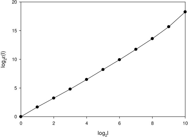
Figure 2: $\log_{2}\epsilon_{\infty}(l)$ vs $\log_{2}l$ for the BCT forest fire model with $L=1024$ and $p=0.0003$

We start with the higher-order moments given by

$$M_{q}(l)=<m(l)^{q}>,$$ (3)

where $m(l)$ is the number of fires contained in a box of linear size $l$; we emphasize that the average is again over all the boxes that contain fires. Following Dubrulle’s analysis of generalized scale covariance and ESS in turbulence Dubrulle , we consider the normalized variables, defined by $\pi(l)=m(l)/\epsilon_{\infty}(l)$, where $\epsilon_{\infty}(l)$ given by

$$\epsilon_{\infty}(l)=\lim_{q\rightarrow\infty}\frac{M_{q+1}(l)}{M_{q}(l)}.$$ (4)

We focus on these normalized variables and calculate their moments, defined as

$$\Pi_{q}(l)=<\pi(l)^{q}>.$$ (5)

We will show numerically that the scaling behavior of $\{\Pi_{q}\}$ is consistent with the Log-Poisson statistics. Let $\pi(l)=\beta^{j}$. If $j$ is a random variable described by a Poisson distribution $P_{l}(j)=\frac{\lambda_{l}^{j}e^{-\lambda_{l}}}{j!}$, then $\pi(l)$ is described by a Log-Poisson distribution. The moments of $\pi(l)$ can then be written as

$$\Pi_{q}(l)=\sum_{j=0}\beta^{qj}\frac{\lambda_{l}^{j}e^{-\lambda_{l}}}{j!}=\exp[\lambda_{l}(\beta^{q}-1)].$$ (6)

It is easy to see that the moments from this Log-Poisson distribution are related by

$$\Pi_{q}(l)=\Pi_{p}(l)^{\zeta(q)/\zeta(p)}=\Pi_{1}(l)^{\zeta(q)},$$ (7)

where

$$\zeta(q)=(1-\beta^{q})/(1-\beta).$$ (8)

Note that $\zeta(q)$ is not linear in $q$ as would be the case for simple scaling. The moments of the original variables $m(l)$ are given by

$$M_{q}(l)=\epsilon_{\infty}^{q}(l)\Pi_{1}(l)^{\zeta(q)}.$$ (9)

To test whether the moments can be described by the Log-Poisson distribution numerically, we first fit the data $M_{q}(l)$ to the above expression. The actual fitting is done using the following expression:

$$\log_{2}(M_{q+1}(l)/M_{q}(l))=a(l)+b(l)\beta^{q},$$ (10)

where $a(l)=\log_{2}\epsilon_{\infty}(l)$ and $b(l)=\log_{2}(\Pi_{1}(l))$. We first determine $\beta$ as follows: For each value of $l$ we do a linear fitting of $\log_{2}(M_{q+1}(l)/M_{q}(l))$ vs $\beta^{q}$, and calculate the overall error, which depends on $\beta$. The best value of $\beta$, corresponding to the minimum overall error, is found to be $\beta\approx 0.75$. With $\beta$ fixed to this value, we find $a(l)$ or $\epsilon_{\infty}(l)$ from the fitting; this is plotted in Fig. 2.

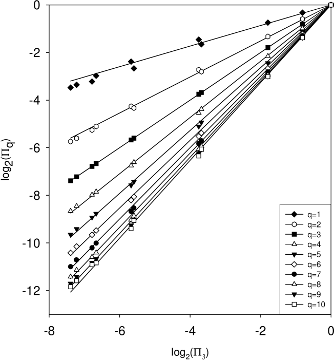
Figure 3: $\Pi_{q}$ vs $\Pi_{3}$. The lines are drawn with slopes $\zeta_{q}/\zeta_{3}$, where $\zeta_{q}$ are defined in Eq. 8. The value of $\beta=0.75$ is chosen as explained in the text.

For $l<\xi$ ($\xi$ is about $2^{8}$ for the value of the parameter $p=0.0003$ used in the simulation), $\epsilon_{\infty}(l)\sim l^{1.8}$. Note that if the original variable $m(l)$ is defined as the density of fires ( instead of the number of fires) in a box of linear size $l$, $\epsilon_{\infty}(l)$ will be approximately given by $l^{1.8}l^{-3}=l^{-1.2}$ — but the normalized variables remain the same. Given $\epsilon_{\infty}(l)$ we can evaluate the normalized moments $\Pi_{q}(l)$. If the distribution is Log-Poisson, then $\Pi_{q}$ vs $\Pi_{p}$ in the log-log plot should fall on a straight line with a slope given by $\zeta(q)/\zeta(p)$. Fig. 3 shows $\Pi_{q}$ vs $\Pi_{3}$ for $q=1,2,\cdots,10$.

Indeed, we find straight lines in the log-log plots with slopes matching $\zeta(q)/\zeta(3)$. This is extended self-similarity (in the normalized variables) for the forest fire model. This is particularly interesting, given the fact that there is actually no scaling regime in the plot of $M_{q}(l)$ or $\Pi_{q}(l)$ vs $l$. The Log-Poisson distribution provides an excellent description of the normalized moments.

4 Extended Self-Similarity in Models of Directed Percolation

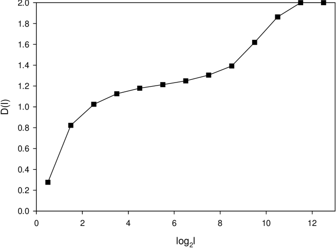
Figure 4: $D(l)$ vs $\log_{2}l$ for $2+1$ DP model with $L=8192$ and $p=0.28734$. $5\times 10^{5}$ time steps (after skipping $100,000$ time steps) were used to obtain the averages.

It is of interest to determine whether the two properties of the forest fire model described in the previous section are displayed by other models. The first, the special form of the scale-dependent dimension appears to be unique to the forest fire model; so far we have not found other types of models which exhibit similar scaling in the first moment. However, the second property of extended self-similarity in normalized variables as described in the last section appears to be much more general. Since the fire propagates and spreads in the background of trees which has presumably a hierarchical and certainly a dynamically changing topology it is interesting to consider simpler models which describe a spreading process. The most obvious one is the well-studied model of directed percolation (DP). dp We found to our surprise that quite a few models of directed percolation (DP) and their variants exhibit a similar form of ESS based on log-Poisson statistics. As an example we consider $2+1$ DP in the supercritical phase $p>p_{c}$, which is very different from the 3d forest fire model. Fig. 4 shows $D(l)$ vs $l$ for this model. Here we use a lattice of size $8192\times 8192$ and $p=0.28734$. Over half millions time steps were used to obtain the averages.

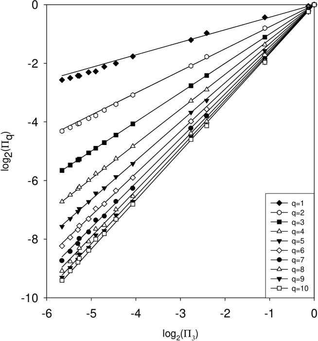
Figure 5: $\Pi_{q}$ vs $\Pi_{3}$ for $2+1$ DP model. The lines are drawn with slopes $\zeta_{q}/\zeta_{3}$, where $\zeta_{q}$ are defined in Eq. 8. The value of $\beta=0.76$ is used.

There is an approximately scale-invariant regime corresponding to $D(l)$ being constant, in contrast to the 3d forest fire model. However, the normalized higher order moments can still be described the Log-Poisson statistics (with $\zeta_{q}$ defined in Eq. 8) and the associated ESS, as can be seen from Fig. 5. This data provides evidence that either the model studied or a model in its vicinity in parameter space exhibits the behavior displayed asymptotically; the proximity to the appropriate fixed point controls this behavior and elucidating its features would be of interest.

5 Summary

We presented extensive numerical evidence to show that the BCT forest fire model exhibits two interesting properties: a logarithmic scale-dependent dimension and Log-Poisson distribution of normalized variables (with $\zeta_{q}$ not linear in $q$) and associated extended self-similarity. The former is likely a unique feature of the forest fire and closely related models; the latter, however, appears to be more general. We have shown that models based on directed percolation also exhibit Log-Poisson statistics (for appropriately normalized variables) similar to that in the forest fire model. This suggests that the Log-Poisson distribution and the associated ESS can be used to describe scaling in a wide range of driven dissipative systems. We hope that studying simple models such as the forest fire model will provide us with some intuition and physical pictures that might eventually be useful for understanding the statistics of energy dissipation and scaling in fully developed turbulence.

This work was supported by the National University of Singapore research grant R-151-000-028-112. KC thanks Maya Paczuski, Peter Grassberger, and Itamar Procaccia for helpful discussions. This work was originally initiated by Per Bak, who was very interested in scaling and ESS in turbulence. He had hoped that a physical picture for ESS could emerge in a simple dynamical model such as the forest fire model. It is sad that he is not around to offer his unique insight on these topics. For many, particularly those who worked closely with him, his premature death has left a big void.

References

- (1) P. Bak, K. Chen, and C. Tang, Phys. Lett. A 147, 297 (1990).
- (2) K. Chen and P. Bak, Phys. Rev. E, 62, 1613 (2000)
- (3) P. Bak and K. Chen, Phys. Rev. Lett., 86, 4215 (2001).
- (4) R. Benzi, S. Ciliberto, R. Tripiccione, C. Baudet, F. Massaioli, S. Succi, Phys. Rev. E, 48, R29 (1993).
- (5) B. Dubrulle, Phys. Rev. Lett. 73, 959 (1994).
- (6) A. N. Kolmogorov, Dokl. Akad. Nauk. SSSR 30, 9 (1941).
- (7) U. Frisch, Turbulence, (Cambridge, New York, 1995).
- (8) K. R. Sreenivasan and P. Kailasanath, Phys. Fluids A 5, 512 (1993).
- (9) A. N. Kolmogorov, J. Fluid Mech. 13, 82 (1962); A. M. Obukhov, J. Fluid Mech. 13, 77 (1962).
- (10) G. Parisi and U. Frisch, in Turbulence and Predictability, Varenna Summer School, edited by M. Ghol, R. Benzi, and G. Parisi, North-Holland, p. 84 (1985).
- (11) Z. S. She and E. Lévêque, Phys. Rev. Lett. 72, 336 (1994).
- (12) For a mean-field approach, see V. Yakhot, Phys. Rev. Lett., 87, 234501, (2001).
- (13) H.-M. Bröker and P. Grassberger, Phys. Rev. E, 56, R4918 (1997).
- (14) K. Chen and P. Bak, Physica A, 321, 256 (2003).
- (15) W. Kinzel, Phase transitions of cellular automata, Z. Phys. B, 58, 229 (1985); P. Grassberger, Directed percolation: results and open problems, in “Nonlinearities in complex systems, proceedings of the 1995 Shimla conference on complex systems”, edited by S. Puri et al, Narosa Publishing, New Delhi(1997)