Dynamics of Social Diversity

Abstract

We introduce and solve analytically a model for the development of disparate social classes in a competitive population. Individuals advance their fitness by competing against those in lower classes, and in parallel, individuals decline due to inactivity. We find a phase transition from a homogeneous, single-class society to a hierarchical, multi-class society. In the latter case, a finite fraction of the population still belongs to the lower class, and the rest of the population is in the middle class, on top of which lies a tiny upper class. While the lower class is static and poor, the middle class is upwardly mobile.

A distinguishing feature of developed societies is the existence of social classes. What accounts for this diversity? Do individuals advance their position as a result of innate talent, inherited wealth, or plain luck? Our aim is to construct a minimalist interacting agent model that accounts for the development of social diversity.

The phenomenon of social diversity has been extensively investigated both in the social C ; G and the biological sciences L ; W . Social hierarchies have been observed empirically in a wide range of animal populations, from insects W1 to mammals A , and to primates VS and humans C1 . An appealing route for modeling social dynamics is to use interacting agent systems vfh ; ckfl . Quantitative ww and large scale simulations bes of physics-inspired interacting particle systems have been used to model observed macroscopic collective phenomena using microscopic agent interactions wdan ; bkr ; smo .

Motivated by empirical observations of bumblebee communities VH , Bonabeau et al. recently introduced an agent-based model of social diversity BTD where each individual is endowed with a fitness-like variable that evolves by two opposing processes. The first is competition: when two agents interact, one individual becomes more fit (gains status) and the other becomes less fit, with the initially fitter individual being more likely to win. Counterbalancing the competition, the winning probability for the fitter agent decreases as the time from the last competition increases. Investigations of this model have found a transition from a homogeneous to a hierarchical society as the relative strengths of these two processes are varied BTD ; SS ; MSK .

In this letter, we introduce a simplified version of the Bonabeau social diversity model that accounts for the competing processes of advancement by competition and decline by inactivity via a single parameter. By solving the underlying rate equations, we find a phase transition from a homogeneous, single-class society to a hierarchical, multi-class society. In the latter phase, the lower class is destitute and static while the middle class is dynamic and has a continuous upward mobility.

In our model, an agent is endowed with an integer fitness value $k\geq 0$. All agents start with zero fitness and the fitness changes by two processes: (i) advancement by competition and (ii) decline by inactivity. In the competition step, when two agents interact, their fitness changes according to

$$(k,j)\to(k+1,j),$$ (1)

for $k\geq j$. When two equally fit agents compete, only one advances. Without loss of generality, the rate of this process is set to one. We also consider the mean-field limit where any pair of agents is equally likely to interact. The rationale behind this “rich gets richer” dynamics is obvious: fitter individuals are better suited for, and hence benefit from, competition. When decline occurs, individual fitness decreases as

$$k\to k-1$$ (2)

with a rate $r$. This process reflects the natural tendency for social status to decrease in the absence of interactions. The lower limit for the fitness is $k=0$; once an individual reaches zero fitness, there is no further decline. The model is characterized by a single parameter, the rate of decline $r$.

Let $f_{k}(t)$ be the fraction of agents with fitness $k$ at time $t$. This distribution obeys the nonlinear master equation

$$\frac{df_{k}}{dt} = r(f_{k+1}-f_{k})+f_{k-1}F_{k-1}-f_{k}F_{k}$$ (3)

for $k\geq 0$, where $F_{k}=\sum_{j=0}^{k}f_{j}$ is the cumulative distribution. The boundary condition is $f_{-1}=0$ so that $df_{0}/dt=rf_{1}-f_{0}^{2}$, and the initial condition is $f_{k}(0)=\delta_{k,0}$. The first two terms in Eq. (3) account for the decline of the fitness of an agent, while the last two terms account for advancement bkm .

To understand the behavior of this system, we focus on the cumulative distribution $F_{k}$, from which the individual densities are $f_{k}=F_{k}-F_{k-1}$. From the master equation (3), the cumulative distribution satisfies

$$\frac{dF_{k}}{dt}=r(F_{k+1}-F_{k})+F_{k}(F_{k-1}-F_{k}),$$ (4)

for $k\geq 0$. The boundary condition is $F_{-1}=0$ so that $dF_{0}/dt=r(F_{1}-F_{0})-F_{0}^{2}$, and the initial condition is $F_{k}(0)=1$.

Homogeneous vs. Hierarchical Societies. Our social diversity model undergoes a phase transition from a homogeneous to a hierarchical society. This transition follows from the continuum limit of the master equation (4) for the cumulative distribution

$$\frac{\partial F}{\partial t}=(r-F)\frac{\partial F}{\partial k}.$$ (5)

For finite fitness, the cumulative distribution approaches a steady state in the long-time limit. Then either $F=r$ or $\partial F/\partial k=0$. Invoking the bound $F\leq 1$, we conclude that either $F=r$ or $F=1$. Therefore, $L$, the fraction of the population with finite fitness exhibits a phase transition

$$L=\begin{cases}r&r<1;\\ 1&r\geq 1.\end{cases}$$ (6)

When competition is weak, the entire population has a finite fitness, while for strong competition, only a fraction $L<1$ of the population has a finite fitness.

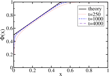
Figure 1: The middle class. The scaled cumulative distribution $\Phi(x)$ versus $x$ for $r=1/2$ at $t=250$ (dotted), $1000$ (dashed), $4000$ (dot-dashed). The solid line is the theoretical prediction (8). The inset shows the qualitative behavior for $r=0$ (dashed), $r\approx 1/2$ (solid), and $r\approx 1$ (dotted).

We shall see that the quantity $L$ is the size of the lower class, while the complementary fraction $1-L$ is the size of the middle class, whose fitness increases indefinitely. Thus for $r\geq 1$, the society is homogeneous and consists of a single lower class. However for $r<1$, there is a hierarchical society that contains a distinct lower class, and a distinct a middle class. When $r=0$, the lower class disappears entirely.

Middle Class Dynamics. The picture presented above is confirmed by analyzing the dynamics of the middle class. Applying dimensional analysis to the governing Eq. (4) suggests that the characteristic fitness of the middle class increases linearly with time, $k\sim t$. Thus, we posit the scaling form

$$F_{k}\simeq\Phi(k/t)$$ (7)

with the boundary condition $\Phi(\infty)=1$. Substituting Eq. (7) into (5), the scaling function satisfies $x\,d\Phi/dx=(\Phi-r)\,d\Phi/dx$ where $x=k/t$. The solution is either $\Phi(x)=r+x$ or $d\Phi/dx=0$. As a result (Fig. 1)

$$\Phi(x)=\begin{cases}r+x&x<1-r;\\ 1&x\geq 1-r.\end{cases}$$ (8)

Remarkably, the scaling function for the cumulative distribution is piecewise linear and thus non-analytic.

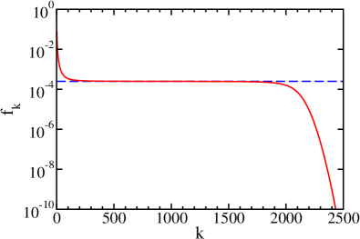
Figure 2: The lower, middle, and upper classes. The fitness distribution $f_{k}$ versus $k$ for $r=1/2$ at $t=4000$ (solid line), showing the lower ($k\lesssim 60$), middle, and upper ($k\gtrsim 2000$) classes. Also shown for reference is the plateau $f_{k}=1/t$ (dashed line). The distribution decays as $1/k^{2}$ in the lower class up to the diffusive scale $k_{\rm lower}\sim(2rt)^{1/2}$. The distribution is constant in the middle class up to a ballistic scale $k_{\rm upper}=(1-r)t$, beyond which there is an upper class that has a Gaussian decay.

The scaling function (8) has a number of basic implications. First, the quantity $\Phi(0)=r$ is the fraction of the population that belongs to the lower class, confirming the prediction of Eq. (6). This behavior is reminiscent of a physical Bose condensate, where a finite fraction of the population occupies the zero fitness (in scaled units) ground state. In this sense, the entire lower class is destitute. When there is only competition ($r=0$), the society consists of a continuously-improving middle class. In this case, a formal exact solution of the master equations is possible unpub .

We can alternatively write the fitness distribution in the scaling form $f_{k}\simeq t^{-1}\phi(k/t)$. The corresponding scaling function is $\phi(x)=d\Phi/dx=r\delta(x)+1$ for $x\leq 1-r$ and $\phi(x)=0$ otherwise. The middle class thus has a constant fitness distribution

$$f_{k}\simeq t^{-1},$$ (9)

for $k<k_{\rm upper}=(1-r)t$. The lot of the middle class is constantly improving, as the fitness extends over a growing range and the average fitness increases linearly with time.

Numerical integration of the master equation confirms these predictions (Figs. 1 and 2). We used a fourth-order Adams-Bashforth method zwillinger with accuracy to $10^{-10}$ in the distribution $F_{k}$. Our numerical data was obtained by integrating $F_{k}$ for $0\leq k<20000$.

Lower Class Dynamics. The fitness of the lower class is finite; in other words, the fitness distribution is in a steady state. This distribution can be determined by setting the time derivative in the rate equation to zero. Writing $F_{k}=L(1-G_{k})$, so that the deviation $G_{k}$ vanishes at large $k$, Eq. (4) gives

$$r\,\frac{G_{k+1}-G_{k}}{G_{k}-G_{k-1}}=L(1-G_{k}).$$ (10)

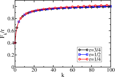
Figure 3: The lower class. The cumulative distribution, normalized by the rate $r$, $F_{k}/r$ is plotted versus $k$. Shown are simulation results for $r=1/4$ (circles), $r=1/2$ (squares), $r=3/4$ (diamonds) at time $t=10^{4}$.

The fitness distribution is fundamentally different in the two phases. In the homogeneous society phase ($r\geq 1$ and $L=1$), the deviation $G_{k}$ decays rapidly at large fitness. Replacing the right-hand side of Eq. (10) by $1$ for large $k$, the solution is simply $G_{k}\sim r^{-k}$. Therefore

$$f_{k}\sim r^{-k}.$$ (11)

The fitness distribution decays exponentially, so that the lower class is confined to a small range of fitness values. The characteristic fitness $1/\ln r$ diverges as the transition is approached. The society is homogeneous as it contains a single social class, the lower class, that does not evolve with time.

In the hierarchical society phase, (where $r<1$ and $L=r$), the fitness distribution is universal, as the recursion relation (10) becomes $r$-independent, $(G_{k+1}-G_{k})/(G_{k}-G_{k-1})=1-G_{k}$. This shows that $F_{k}/r$ is a universal, $r$-independent distribution (Fig. 3). We start by treating $k$ as a continuous variable, because the fitness range becomes large as $r\downarrow 1$. We thus expand the differences in Eq. (10) to second order. Since $G^{\prime\prime}\ll G^{\prime}$, where prime denotes differentiation with respect to $k$, we find $G^{\prime\prime}+GG^{\prime}=0$. Integrating once and invoking $G\to 0$ as $k\to\infty$, gives $G^{\prime}+\frac{1}{2}G^{2}=0$. Asymptotically, $G\simeq 2k^{-1}$, and then by using $f_{k}=F_{k}-F_{k-1}$, we find

$$f_{k}\simeq 2r\,k^{-2}.$$ (12)

The lower class has a power-law fitness distribution with mean fitness that diverges logarithmically in the upper limit. While the lower class is still static, it is not as destitute as in the homogeneous society phase.

The transition between the lower and middle class occurs when $2r/k^{2}\approx 1/t$, i.e., where the power-law distribution (12) matches the uniform distribution (9). Consequently, the lower class is confined to a diffusive boundary layer of thickness

$$k_{\rm lower}\sim(2rt)^{1/2}.$$ (13)

Beyond this diffusive scale, lies the middle class whose constant density (9) extends over the range $k_{\rm lower}<k<k_{\rm upper}$. In the hierarchical society phase, the fitness distribution consists of the stationary component (12) that defines the lower class and the evolving component (7) that defines the middle class. The extent of the stationary region indefinitely grows with time.

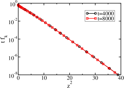
Figure 4: The upper class. Shown is the normalized tail of the fitness distribution: $tf_{k}$ versus $z^{2}$, with the scaling variable $z=(k-vt)/\sqrt{Dt}$, for $r=1/2$ at times $t=4000$ (circles) and $t=8000$ (squares).

We thus conclude that the lower class is always static, being in a steady-state independent of the rate of decline $r$. In a homogeneous society, the lower class has an exponentially decaying fitness distribution that lies within a narrow fitness range. In a hierarchical society, the lower class fitness distribution decays algebraically and its range grows diffusively with time.

Upper Class Dynamics. The upper class is defined by the subpopulation whose fitness lies beyond $k_{\rm upper}=(1-r)t$. We probe the tail of this fitness distribution by again considering the deviation $G_{k}$, defined by $F_{k}=1-G_{k}$. This deviation obeys the convection-diffusion equation

$$\frac{\partial G_{k}}{\partial t}+v\frac{\partial G_{k}}{\partial k}=D\frac{\partial^{2}G_{k}}{\partial k^{2}}$$ (14)

with upward drift velocity $v=(1-r)$ and diffusion coefficient $D=(1+r)/2$. The boundary condition $G(k=vt)\propto t^{-1}$ is set by matching the density at the top of the middle class with that at the bottom of the upper class. Consequently, the fitness distribution, $f=-\partial G/\partial k$, follows the scaling form (Fig. 4)

$$f_{k}(t)\simeq t^{-1}\psi\left(\frac{k-vt}{\sqrt{Dt}}\right),$$ (15)

where the scaling function has the Gaussian tail $\psi(z)\sim\exp(-z^{2}/2)$, as $z\to\infty$.

The upper class is thus confined to a diffusive boundary layer that grows as $\sqrt{Dt}$. From Eq. (15), the upper class contains a fraction $\propto 1/\sqrt{t}$ of the total population. Finally, for a finite population of $N$ agents, we deduce from the extreme statistics criterion, $Nf_{k}\sim 1$, that for the fittest agent $k_{\rm extreme}\sim vt+\sqrt{t\ln N}$.

We comment that the deceptively simple master equation exhibits a remarkable triple-deck structure, with a stationary component, followed by two transient components. Interestingly, the asymptotic fitness distribution is described by a non-analytic scaling function.

In summary, we introduced a minimal model of social diversity in which the two driving mechanisms are advancement by competition and decline by inactivity. An idealized but plausible social structure emerges: either a homogeneous society with a single lower class, or a hierarchical society with multiple classes. The lower class is always static, while the middle class and the (tiny) upper classes are upwardly mobile. In a hierarchical society, the lower and the upper classes are confined to boundary layers that are much smaller than the dominant scale that characterizes the fitness of the middle class.

There are numerous interesting questions suggested by this work. For example, what is the time history of an individual? How rigid is the social hierarchy and how does it depend on the population size? What happens if each individual is also endowed with an intrinsic fitness? Last, does non-trivial spatial organization emerge when agents move locally in space?

We thank D. Stauffer for stimulating our interest in social diversity, K. Kulakowski for an informative discussion, and D. Watts for literature advice. We also acknowledge financial support from DOE grant W-7405-ENG-36 (EB and SR) and NSF grant DMR0227670 (SR).

References

- (1) I. D. Chase, Amer. Sociological Rev. 45, 905 (1980).
- (2) R. V. Gould, Amer. J. Sociology 107, 1143 (2002).
- (3) H. G. Landau, Bull. Math. Biophys. 13, 1 (1951).
- (4) E. O. Wilson, Sociobiology, (Harvard University Press, Cambridge, MA, 1975).
- (5) E. O. Wilson, The Insect Societies, (Harvard University Press, Cambridge, MA, 1971).
- (6) W. C. Allee, Biol. Symp. 8, 139 (1942); A. M. Guhl, Anim. Behav. 16, 219 (1968); M. W. Schein and M. H. Forman, Brit. J. Anim. Behav. 3, 45 (1955).
- (7) M. Varley and D. Symmes, Behaviour 27, 54 (1966).
- (8) I. Chase, Behav. Sci. 19, 374 (1980).
- (9) D. Helbing, I. Farkas, and T. Vicsek, Nature 407, 487 (2000).
- (10) I. D. Couzin, J. Krause, N. R. Franks, S. A. Levin, Nature 433, 513 (2005).
- (11) W. Weidlich, Sociodynamics: A Systematic Approach to Mathematical Modelling in the Social Sciences (Harwood Academic Publishers, 2000).
- (12) C. L. Barrett, S. G. Eubank, and J. P. Smith, Scientific American 292, 54 (2005).
- (13) G. Weisbuch, G. Deffuant, F. Amblard, and J. P. Nadal, Complexity 7, 55 (2002).
- (14) E. Ben-Naim, P. L. Krapivsky, and S. Redner, Physica D 183, 190 (2003).
- (15) D. Stauffer and H. Meyer-Ortmanns, Int. J. Mod. Phys. B 15, 241 (2004).
- (16) C. Van Honk and P. Hogeweg, Behav. Ecol. Sociobiol. 9, 111 (1981).
- (17) E. Bonabeau, G. Theraulaz, and J.-L. Deneubourg, Physica A 217, 373 (1995).
- (18) A. O. Sousa and D. Stauffer, Intl. J. Mod. Phys. C 5, 1063 (2000).
- (19) K. Malarz, D. Stauffer, and K. Kulakowski, preprint.
- (20) Rate equations of a similar structure were obtained in a study of the statistics of random binary trees. See E. Ben-Naim, P. L. Krapivsky, and S. N. Majumdar, Phys. Rev. E 64, R035101 (2000).
- (21) E. Ben-Naim and S. Redner, unpublished.
- (22) D. Zwillinger, Handbook of Differential Equations (Academic Press, London, 1989).