Generalized Geometric Cluster Algorithm for Fluid Simulation

Abstract

We present a detailed description of the generalized geometric cluster algorithm for the efficient simulation of continuum fluids. The connection with well-known cluster algorithms for lattice spin models is discussed, and an explicit full cluster decomposition is derived for a particle configuration in a fluid. We investigate a number of basic properties of the geometric cluster algorithm, including the dependence of the cluster-size distribution on density and temperature. Practical aspects of its implementation and possible extensions are discussed. The capabilities and efficiency of our approach are illustrated by means of two example studies.

I Introduction

Computer simulation methods play an increasingly important role in the study of complex fluids. Historically, many simulations have concentrated on fluids modeled as an assembly of monodisperse spherical particles interacting, e.g., via a bare excluded-volume potential (hard-sphere fluid) or a Lennard-Jones interaction Allen and Tildesley (1987). While such systems can already display a wealth of interesting features, such as a solid–liquid transition and—in the presence of attractive interactions—a critical point, it is also clear that real fluids and solutions can exhibit far richer behavior. Various factors contribute to the additional features found in these systems, including internal degrees of freedom of the constituents (such as in polymeric systems), interactions induced by electrical charges, and the presence of various species with a strong size asymmetry. Modeling any of these properties can greatly increase the required numerical efforts and in certain situations can make the simulations prohibitively expensive. Although available computational power continues to increase steadily, further progress in simulating such systems will critically depend on algorithmic advances.

Recently, we have introduced a simulation method that addresses one of the above-mentioned complicating factors, namely the slow-down arising in simulations of solutions containing species of largely different sizes Liu and Luijten (2004a) (see also Ref. Day (2004)). This method, which generalizes an original idea due to Dress and Krauth Dress and Krauth (1995) to identify clusters based upon geometric symmetry operations and accordingly is called the (generalized) geometric cluster algorithm (GCA), exhibits two noteworthy features. Firstly, it employs a nonlocal Monte Carlo (MC) scheme to move the constituent particles in a nonphysical way, thus introducing artificial dynamics while preserving all thermodynamic equilibrium properties. This greatly accelerates the generation of uncorrelated configurations of particles. We emphasize that our scheme does not involve any approximations; the molecular configurations produced by the GCA are generated according to the same Boltzmann distribution that would govern a conventional simulation of the system under consideration, but the GCA follows a different trajectory through phase space. Secondly, the nonlocal moves involve clusters of particles that are constructed in such a way that all proposed moves are accepted. This is not only an additional factor contributing to the efficiency of the method, but it also has a more profound significance. Namely, in order to satisfy detailed balance Gubernatis (2003); Landau and Binder (2000); Frenkel and Smit (2002); Newman and Barkema (1999) without imposing the usual Metropolis Metropolis et al. (1953) acceptance criterion, the ratio of the probability of transforming a particle configuration $C$ into a new configuration $C^{\prime}$ and the probability of the reverse transformation must be identical to the ratio of the Boltzmann factors of the configuration $C^{\prime}$ and the original configuration $C$. Clearly, this can only be realized if the transformations (“moves”) are proposed with a probability that involves knowledge about the physical properties of a system. For the vast majority of MC algorithms, this is not the case. The most well-known exceptions are the Swendsen–Wang (SW) algorithm Swendsen and Wang (1987) for lattice spin models and its variant due to Wolff Wolff (1989). Among continuum systems, hard-sphere fluids constitute a special case, since all configurations without particle overlap have the same energy and thus the same Boltzmann factor. However, it is generally accepted that these rejection-free algorithms are an exception (cf., e.g., Ref. Frenkel and Smit (2002), Sec. 14.3.1). Indeed, ever since the invention of the SW cluster algorithm for Ising and Potts models, its extension to fluids has been a widely-pursued goal. For lattice gases the extension can be accomplished in a straightforward manner, since they are isomorphic to Potts models. However, for off-lattice (continuum) fluids, this mapping cannot be applied, owing to the absence of particle–hole symmetry. This symmetry is a critical ingredient for the SW algorithm for Ising and Potts models, as clusters of spins (or variables, in the case of the Potts model) are identified using a symmetry operation that, if applied globally, would leave the Hamiltonian of the system invariant. The only known extensions to continuum systems apply to the Widom–Rowlinson model for fluid mixtures Johnson et al. (1997); Chayes and Machta (1998), in which identical particles do not interact and unlike species experience a hard-core repulsion, and the closely-related Stillinger–Helfand model, in which the hard-core is replaced by a soft repulsion Sun et al. (2000). However, no generalization has been found in which identical particles do not behave as an ideal gas. In a separate development, Dress and Krauth Dress and Krauth (1995) observed that, for hard-core fluids, an overlap-free configuration can be transformed into a new configuration of nonoverlapping particles by means of a geometric symmetry operation. The particular advantage of this scheme is its ability to efficiently relax size-asymmetric mixtures Buhot and Krauth (1998); Santen and Krauth (2000); Malherbe and Amokrane (2001). In Ref. Liu and Luijten (2004a) we showed how this advantage can be retained for fluids with arbitrary pair potentials, while simultaneously exploiting the invariance of the Hamiltonian under the symmetry operation to create particle clusters in a manner that is fully analogous to the SW or Wolff method. An application to a concrete physical problem has been presented in Ref. Liu and Luijten (2004b), where colloid–nanoparticle mixtures featuring attractive, repulsive and hard-core interactions were simulated for size asymmetries up to 100. We remark that geometric cluster algorithms have also been applied successfully to lattice-based models. Heringa and Blöte have employed it to investigate lattice gases with nearest-neighbor exclusion Heringa and Blöte (1996) and developed a version for simulation of the Ising model in the constant-magnetization ensemble Heringa and Blöte (1998a). The “pocket algorithm” of Krauth and Moessner Krauth and Moessner (2003), which is essentially a geometric cluster algorithm for dimer models, was used to investigate hard-core dimers on three-dimensional lattices Huse et al. (2003). Furthermore, we note that there is a profound difference between the geometric cluster algorithm and other Monte Carlo schemes that move groups of particles simultaneously Wu et al. (1992); Jaster (1999); Lue and Woodcock (1999); Lobaskin and Linse (1999). Such algorithms can work efficiently in specific cases, and are sometimes viewed as counterparts of the SW algorithm merely because they also invoke the notion of a “cluster,” but they typically involve a tunable parameter and are neither rejection free nor do they exploit a symmetry property of the Hamiltonian.

In the current article we provide a detailed description of the generalized geometric cluster algorithm for continuum fluids and study basic properties such as the dependence of cluster-size distribution on temperature and density. We also describe a multiple-cluster variant of the generalized GCA in which a particle configuration is fully decomposed into clusters that can be moved independently.

II Algorithm description

II.1 Swendsen–Wang and Wolff algorithms for lattice spin models

For reference in future sections that highlight the similarities between the generalized GCA Liu and Luijten (2004a) for off-lattice fluids and the SW Swendsen and Wang (1987) and Wolff Wolff (1989) algorithms for lattice spin models, we briefly summarize the lattice cluster algorithms for the case of a $d$-dimensional Ising model with nearest-neighbor interactions, described by the Hamiltonian

$$\mathcal{H}_{\rm Ising}=-J\sum_{\langle ij\rangle}s_{i}s_{j}\;.$$ (1)

The spins $s$ are placed on the vertices of a square ($d=2$) or simple cubic ($d=3$) lattice and take values $\pm 1$. The sum runs over all pairs of nearest neighbors, which are coupled via a ferromagnetic coupling with strength $J>0$. Starting from a given configuration of spins, the SW algorithm now proceeds as follows:

1. A “bond” is formed between every pair of nearest neighbors that are aligned, with a probability $p_{ij}=1-\exp(-2\beta J)$, where $\beta=1/k_{\rm B}T$.

2. All spins that are connected, directly or indirectly, via bonds belong to a single cluster. Thus, the bond assignment procedure divides the system into clusters of parallel spins. Note how the bond probability (and hence the typical cluster size) grows with increasing coupling strength $\beta J$ (decreasing temperature). For finite $\beta J$, $p_{ij}<1$ and hence a cluster is generally a subset of all spins of a given sign.

3. All spins in each cluster are flipped collectively with a probability $\frac{1}{2}$. I.e., for each cluster of spins a spin value $\pm 1$ is chosen and this value is assigned to all spins that belong to the cluster.

The last, and crucial, step is made possible by the Fortuin–Kasteleyn mapping Kasteleyn and Fortuin (1969); Fortuin and Kasteleyn (1972) of the Potts model on the random-cluster model, which implies that the partition function of the former can be written as a Whitney polynomial that represents the partition function of the latter Baxter et al. (1976). Accordingly, all spins in a cluster (a connected component in the random-cluster model) are uncorrelated with all other spins, and can be assigned a new spin value.

This algorithm possesses several noteworthy properties. First, it strongly suppresses dynamic slowing down near a critical point Swendsen and Wang (1987) by efficiently destroying nonlocal correlations (see also Ref. Newman and Barkema (1999) for a pedagogical introduction). Secondly, this algorithm is rejection free. Indeed, the assignment of bonds involves random numbers, but once the clusters have been formed each of them can be flipped independently without imposing an acceptance criterion involving the energy change induced by such a collective spin-reversal operation. Thirdly, the Fortuin–Kasteleyn mapping can also be applied to systems in which each spin interacts not only with its nearest neighbors, but also with other spins Baxter et al. (1976). In particular, the coupling strength can be different for different spin pairs, leading to a probability $p_{ij}$ that is, e.g., dependent on the separation between $i$ and $j$. Thus, cluster algorithms can be designed for spin systems with medium- Luijten et al. (1996) and long-range interactions Luijten and Blöte (1995).

Critical slowing down is suppressed even more strongly in a variant of this algorithm due to Wolff Wolff (1989). In this implementation, no decomposition of the entire spin configuration into clusters takes place. Instead, a single cluster is formed, which is then always flipped:

1. A spin $i$ is selected at random.

2. All nearest neighbors $j$ of this spin are added to the cluster with a probability $p_{ij}=1-\exp(-2\beta J)$, provided spins $i$ and $j$ are parallel and the bond between $i$ and $j$ has not been considered before.

3. Each spin $j$ that is indeed added to the cluster is also placed on the stack. Once all neighbors of $i$ have been considered for inclusion in the cluster, a spin is retrieved from the stack and all its neighbors are considered in turn for inclusion in the cluster as well, following step 2.

4. Steps 2 and 3 are repeated iteratively until the stack is empty.

5. Once the cluster has been completed, all spins in the cluster are inverted.

Again, this is a rejection-free algorithm, in the sense that the cluster is always flipped. Just as in the SW algorithm, the cluster-construction process involves random numbers, but the individual probabilities $p_{ij}$ involve single-particle energies rather than an acceptance criterion that involves the total energy change induced by a cluster flip.

II.2 Geometric cluster algorithm for hard-sphere mixtures

Since suppression of critical slowing is a highly attractive feature for fluid simulations as well, the generalization of the SW and Wolff algorithms to fluid systems has been a widely-pursued goal. In the lattice-gas interpretation, where a spin $+1$ corresponds to a particle and a spin $-1$ corresponds to an empty site, a spin-inversion operation corresponds to a particle being inserted in or removed from the system. This “particle–hole symmetry” is absent in off-lattice (continuum) systems. While a particle in a fluid configuration can straightforwardly be deleted, there is no unambiguous prescription on how to transform empty space into a particle. More precisely, in the lattice cluster algorithms the operation performed on every spin is self-inverse. This requirement is not fulfilled for off-lattice fluids.

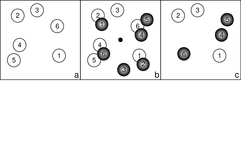
Figure 1: Illustration of the geometric cluster algorithm for hard disks Dress and Krauth (1995). a) Original configuration. b) A new configuration (shaded circles) is created by means of a point reflection of all particles with respect to a randomly-chosen pivot point (small filled disk). The superposition of the original and the new configuration leads to groups of overlapping particles. In this example, there are three pairs of groups ($\{1,2\}$, $\{3\}$, $\{4,5,6\}$). Each pair is denoted a cluster. The particles in any one of these clusters can be point-reflected with respect to the pivot without affecting the other two clusters. This can be used to carry out the point reflection for every cluster with a pre-set probability. c) Final configuration that results if, starting from the original configuration, only the particles in the third cluster $\{4,5,6\}$ are point-reflected. This approach guarantees that every generated configuration will be free of overlaps. Note that the pivot will generally not be placed in the center of the cell, and that the periodic boundary conditions indeed permit any position.

Dress and Krauth Dress and Krauth (1995) proposed a method to efficiently generate particle configurations for a hard-sphere liquid. This geometric cluster algorithm proceeds as follows (cf. Fig. 1).

1. In a given configuration $C$, a “pivot” is chosen at random.

2. A configuration $\tilde{C}$ is now generated by carrying out a point reflection for all particles in $C$ with respect to the pivot.

3. The configuration $C$ and its transformed counterpart $\tilde{C}$ are superimposed, which leads to groups of overlapping particles. The groups generally come in pairs, except possibly for a single group that is symmetric with respect to the pivot. Each pair is denoted a “cluster” not (a).

4. For each cluster, all particles can be exchanged between $C$ and $\tilde{C}$ without affecting particles belonging to other clusters. This exchange is performed for each cluster independently with a probability $\smash{\frac{1}{2}}$. Thus, if the superposition of $C$ and $\tilde{C}$ is decomposed into $N$ clusters, there are $2^{N}$ possible new configurations. The configurations that are actually realized are denoted $C^{\prime}$ and $\tilde{C}^{\prime}$, i.e., the original configuration $C$ is transformed into $C^{\prime}$ and its point-reflected counterpart $\tilde{C}$ is transformed into $\tilde{C}^{\prime}$.

5. The configuration $\tilde{C}^{\prime}$ is discarded and $C^{\prime}$ is the new configuration, serving as the starting point for the next iteration of the algorithm. Note that a new pivot is chosen in every iteration.

Observe that periodic boundary conditions must be employed, such that an arbitrary placement of the pivot is possible. Other self-inverse operations are permissible, such as a reflection in a plane Heringa and Blöte (1996), in which case various orientations of the plane must be chosen in order to satisfy ergodicity. While operating in the canonical rather than in the grand-canonical ensemble, this prescription clearly bears great resemblance to the original SW algorithm. The original configuration is decomposed into clusters by exploiting a symmetry operation that leaves the Hamiltonian invariant if applied to the entire configuration; in the SW algorithm this is the spin-inversion operation and in the geometric cluster algorithm it is a geometric symmetry operation. Subsequently, a new configuration is created by moving each cluster independently with a certain probability.

We note that this method represents an approach of great generality. For example, it is not restricted to monodisperse systems, and has indeed been applied successfully to binary Buhot and Krauth (1998) and polydisperse Santen and Krauth (2000) mixtures. Indeed, the nonlocal character of the particle moves makes them exquisitely suitable to overcome the jamming problems that slow down the simulation of size-asymmetric mixtures. An important limitation of the algorithm is the fact that the average cluster size increases very rapidly beyond a certain density, corresponding to the percolation threshold of the combined system containing the superposition of the configurations $C$ and $\tilde{C}$. Once this cluster spans the entire system, the algorithm is clearly no longer ergodic.

We can take the analogy with the lattice cluster algorithms one step further, by showing that a single-cluster (Wolff) variant can be formulated as well Heringa and Blöte (1996); Liu and Luijten (2004a).

1. In a given configuration $C$, a “pivot” is chosen at random.

2. A particle $i$ is selected as the first particle that belongs to the cluster. This particle is moved via a point reflection with respect to the pivot. In its new position, the particle is referred to as $i^{\prime}$.

3. Step 2 is repeated iteratively for each particle $j$ that overlaps with $i^{\prime}$. Thus, if the (moved) particle $j^{\prime}$ overlaps with another particle $k$, particle $k$ is moved as well. Note that all translations involve the same pivot.

4. Once all overlaps have been resolved, the cluster move is completed.

As in the SW-like prescription, a new pivot is chosen for each cluster that is constructed.

II.3 Geometric cluster algorithm for interacting particles: Single-cluster variant

The geometric cluster algorithm described in the previous section is formulated for hard-core interactions. For application to general pair potentials, it was suggested in Ref. Dress and Krauth (1995) to impose a Metropolis-type acceptance criterion based upon the energy difference induced by the cluster move. Indeed, in the case of potentials that consist of a hard-core (excluded-volume) contribution supplemented by an attractive or repulsive tail, such as a Yukawa potential, the cluster-construction procedure guarantees that no overlaps are generated and the acceptance criterion takes into account the tail of the interactions. For “soft-core” potentials, such as a Lennard-Jones interaction, the situation becomes already somewhat more complicated, since an arbitrary excluded-volume distance must be chosen for the cluster construction. As the algorithm will not generate configurations in which the separation between a pair of particles is less than this distance (i.e., the particle “diameter,” in the case of monodisperse systems), it must be set to a value that is smaller than any separation that would typically occur, as already noted in Ref. Malherbe and Amokrane (1999). In either case, the clusters that are generated have only limited physical relevance, and the evaluation of a considerable part of the energy change resulting from a cluster move is deferred until the acceptance step. Rejection is not only likely, but also costly, given the computational efforts of both cluster construction and energy evaluation. We note that this approach was nevertheless applied to Yukawa mixtures with moderate size asymmetry (diameter ratio $\leq 5$) Malherbe and Amokrane (1999).

On the other hand, Heringa and Blöte Heringa and Blöte (1998a); Heringa and Blöte (1998b) devised an geometric cluster algorithm for the Ising model in which the nearest-neighbor interactions between spins are taken into account already during the cluster construction. While this lattice model can obviously be simulated by the SW and Wolff algorithms, their approach permits simulation in the constant-magnetization ensemble. The geometric operations employed map the spin lattice onto itself, such that excluded-volume conditions are satisfied automatically: every spin move amounts to an exchange of spins. For every spin pair $(i,i^{\prime})$ that is exchanged, each of its nearest-neighbor pairs $(k,k^{\prime})$ are exchanged with a probability that depends on the change in pair energy, $\Delta=(E_{ik}+E_{i^{\prime}k^{\prime}})-(E_{ik^{\prime}}+E_{i^{\prime}k})$. This procedure is then again performed iteratively for the neighbors of all spin pairs that are exchanged.

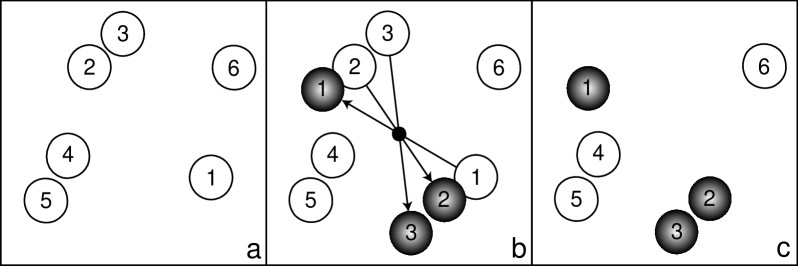
Figure 2: Two-dimensional illustration of the interacting geometric cluster algorithm. Like in Fig. 1, open and shaded disks denote the particles before and after the geometric operation, respectively, and the small disk denotes the pivot. However, in the generalized GCA a single cluster is constructed, to which particles are added with an interaction-dependent probability. a) Original configuration. b) A cluster is constructed as follows. Particle 1 is point-reflected with respect to the pivot. If, in its new position, it has a repulsive interaction with particle 2, the latter has a certain probability to be point-reflected as well, with respect to the same pivot. Assuming an attractive interaction between particles 2 and 3, particle 3 is translated as well, but again only with a certain probability. If particles 4–6 are not affected by these point reflections, the cluster construction terminates. c) The new configuration consists of particles 1–3 in their new positions and particles 4–6 in the original positions. A new pivot is chosen and the procedure is repeated.

In Ref. Liu and Luijten (2004a) we introduced a generalization of the GCA for off-lattice fluids, in which particles undergo a geometric operation in a stochastic manner, akin to the approach of Ref. Heringa and Blöte (1998a). The differences arise from the fact that no underlying lattice is present, so that particles are added to the cluster on an individual basis, rather than in pairs. All interactions are treated in a unified manner, so there is no technical distinction between attractive and repulsive interactions or between hard-core and soft-core potentials. This generalized GCA is most easily described as a combination of the single-cluster methods formulated in Sec. II.1 and II.2. We assume a general pair potential $V_{ij}(\mathbf{r}_{ij})$ that does not have to be identical for all pairs $(i,j)$ (see Fig. 2).

1. In a given configuration $C$, a “pivot” is chosen at random.

2. A particle $i$ at position $\mathbf{r}_{i}$ is selected as the first particle that belongs to the cluster. This particle is moved via a point reflection with respect to the pivot. In its new position, the particle is referred to as $i^{\prime}$, at position $\mathbf{r}_{i}^{\prime}$.

3. Each particle $j$ that interacts with $i$ or $i^{\prime}$ is now considered for addition to the cluster. Unlike the first particle, particle $j$ is point-reflected with respect to the pivot only with a probability $p_{ij}=\max[1-\exp(-\beta\Delta_{ij}),0]$, where $\Delta_{ij}=V(|\mathbf{r}_{i}^{\prime}-\mathbf{r}_{j}|)-V(|\mathbf{r}_{i}-\mathbf{r}_{j}|)$. A particle $j$ that interacts with $i$ both in its old and in its new position is nevertheless treated only once.

4. Each particle $j$ that is indeed added to the cluster (i.e., moved) is also placed on the stack. Once all particles interacting with $i$ or $i^{\prime}$ have been considered, a particle is retrieved from the stack and all its neighbors that are not yet part of the cluster are considered in turn for inclusion in the cluster as well, following step 3.

5. Steps 3 and 4 are repeated iteratively until the stack is empty. The cluster move is now complete.

If a particle interacts with multiple other particles that have been added to the cluster, it can thus be considered multiple times for inclusion. However, once it has been added to the cluster, it cannot be removed. This is an important point in practice, since particles undergo a point reflection already during the cluster construction process (and thus need to be tagged, in order to prevent them from being returned to their original position by a second point reflection). A crucial aspect is that the probability $p_{ij}$ only depends on the change in pair energy between $i$ and $j$. A change in the relative position of $i$ and $j$ occurs if particle $j$ is not added to the cluster. This happens with a probability $1-p_{ij}=\min[\exp(-\beta\Delta_{ij}),1]$. The similarity with the Metropolis acceptance criterion is deceptive (and merely reflects the fact that both algorithms aim to generate configurations according to the Boltzmann distribution) , since $\Delta_{ij}$ does not represent the total energy change resulting from the translation of particle $i$. Instead, other energy changes are taken into account via the iterative nature of the algorithm.

It is instructive to note that the expression for $p_{ij}$ bears close resemblance to the probability employed in the SW algorithm (Sec. II.1). In the latter, two different situations can be discerned that lead to a change in the relative energy $\smash{\Delta_{ij}^{\rm SW}}$ between a spin $i$ that belongs to the cluster and a spin $j$ that does not yet belong to the cluster. If $i$ and $j$ are initially antiparallel, $j$ will never be added to the cluster and only spin $i$ will be inverted, yielding an energy change $\smash{\Delta_{ij}^{\rm SW}}=-2J<0$ that occurs with probability unity. If $i$ and $j$ are initially parallel and $j$ is not added to the cluster, the resulting change in the pair energy equals $\smash{\Delta_{ij}^{\rm SW}}=+2J>0$. This occurs with a probability $\exp(-2\beta J)<1$. These two situations can indeed be summarized as $\min[\exp(-\beta\Delta_{ij}^{\rm SW}),1]$, just as in the generalized GCA.

The ergodicity of this algorithm follows from the fact that there is a nonvanishing probability that a cluster consists of only one particle, which can be moved over an arbitrarily small distance, since the location of the pivot is chosen at random. This obviously requires that not all particles are part of the cluster, a condition that is violated at high packing fractions. While a compact proof of detailed balance of the generalized GCA has already been given in Ref. Liu and Luijten (2004a), we include it here for the sake of completeness. We consider a configuration $X$ that is transformed into a configuration $Y$ by means of a cluster move. All particles included in the cluster maintain their relative separation; as noted above, an energy change arises if a particle is not included in the cluster, but interacts with a particle that does belong to the cluster. Following Wolff Wolff (1989) we denote each of these interactions as a “broken bond.” A broken bond $k$ that corresponds to an energy change $\Delta_{k}$ occurs with a probability $1-p_{k}=1$ if $\Delta_{k}\leq 0$ and a probability $1-p_{k}=\exp(-\beta\Delta_{k})$ if $\Delta_{k}>0$. The formation of an entire cluster corresponds to the breaking of a set $\{k\}$ of bonds, which has a probability $P$. This set is comprised of the subset $\{l\}$ of broken bonds $l$ that lead to an increase in pair energy and the subset $\{m\}$ of broken bonds that lead to a decrease in pair energy, such that

$$P=\prod_{k}(1-p_{k})=\exp\left[-\beta\sum_{l}\Delta_{l}\right]\;.$$ (2)

The transition probability from configuration $X$ to configuration $Y$ is proportional to the cluster formation probability,

$$T(X\to Y)=C\exp\left[-\beta\sum_{l}\Delta_{l}\right]\;,$$ (3)

where the factor $C$ accounts for the fact that various arrangements of bonds within the cluster (“internal bonds”) correspond to the same set of broken bonds. In addition, it incorporates the probability of choosing a particular pivot and a specific particle as the starting point for the cluster.

If we now consider the reverse transition $Y\to X$, we observe that this again involves the set $\{k\}$, but all the energy differences change sign compared to the forward move. Consequently, the subset $\{l\}$ in Eq. (3) is replaced by its complement $\{m\}$ and the transition probability is given by

$$T(Y\to X)=C\exp\left[+\beta\sum_{m}\Delta_{m}\right]\;,$$ (4)

where the factor $C$ is identical to the prefactor in Eq. (3). Since we require the geometric operation to be self-inverse we thus find that the cluster move satisfies detailed balance at an acceptance ratio of unity,

$$\frac{T(X\to Y)}{T(Y\to X)}=\frac{\exp\left[-\beta\sum_{l}\Delta_{l}\right]}{\exp\left[+\beta\sum_{m}\Delta_{m}\right]}=\exp\left[-\beta\sum_{k}\Delta_{k}\right]=\exp\left[-\beta(E_{Y}-E_{X})\right]=\frac{\exp(-\beta E_{Y})}{\exp(-\beta E_{X})}\;,$$ (5)

where $E_{X}$ and $E_{Y}$ are the internal energies of configurations $X$ and $Y$, respectively. I.e., the ratio of the forward and reverse transition probabilities is equal to the inverse ratio of the Boltzmann factors, so that we indeed have created a rejection-free algorithm. This is obscured to some extent by the fact that in our prescription the cluster is moved while it is being constructed, similar to the Wolff algorithm in Sec. II.1. The central point, however, is that the construction solely involves single-particle energies, whereas a Metropolis-type approach only evaluates the total energy change induced by a multi-particle move and then frequently rejects this move. By contrast, the GCA avoids large energy differences by incorporating “offending” particles into the cluster with a high probability.

II.4 Geometric cluster algorithm for interacting particles: Full cluster decomposition

We now introduce a SW implementation of the generalized GCA. The merit of this formulation, which builds upon the Wolff version described in the previous section, is twofold: First, it demonstrates that the algorithm constitutes the true off-lattice counterpart of the SW and Wolff cluster algorithms for spin models outlined in Sec. II.1. Secondly, the SW formulation produces a full decomposition of an off-lattice fluid configuration into stochastically independent clusters. This implies an interesting and remarkable analogy with the Ising model. As observed by Coniglio and Klein Coniglio and Klein (1980) for the two-dimensional Ising model at its critical point, the clusters created according to the prescription in Sec. II.1 are just the so-called “Fisher droplets” Fisher (1967). While Ref. Coniglio and Klein (1980) makes no reference to the work by Fortuin and Kasteleyn, these “Coniglio–Klein clusters” are implied by the Fortuin–Kasteleyn mapping of the Potts model onto the random-cluster model Fortuin and Kasteleyn (1972), which in turn constitutes the basis for the Swendsen–Wang approach Swendsen and Wang (1987). The clusters generated by the GCA do not have an immediate physical interpretation, as they typically consist of two spatially disconnected parts. However, just like the Ising clusters can be inverted at random, each cluster of fluid particles can be moved independently with respect to the remainder of the system. As such, the generalized GCA can be viewed as a continuum version of the Fortuin–Kasteleyn mapping.

The cluster decomposition of a configuration proceeds as follows. First, a cluster is constructed according to the Wolff version of Sec. II.3, with the exception that the cluster is only identified; particles belonging to the cluster are marked but not actually moved. The pivot employed will also be used for the construction of all subsequent clusters in this decomposition. These subsequent clusters are built just like the first cluster, except that particles that are already part of an earlier cluster will never be considered for a new cluster. Once each particle is part of exactly one cluster the decomposition is completed. Like in the SW algorithm, every cluster can then be moved (i.e., all particles belonging to it are translated via a point reflection) independently, e.g., with a probability $f$. Despite the fact that all clusters except the first are built in a restricted fashion, each individual cluster is constructed according to the rules of the Wolff formulation of Sec. II.3. The exclusion of particles that are already part of another cluster simply corresponds to the fact that every bond should be considered only once. If a bond is broken during the construction of an earlier cluster it should not be re-established during the construction of a subsequent cluster. The cluster decomposition thus obtained is not unique, as it depends on the placement of the pivot and the choice of the first particle. Evidently, this also holds for the SW algorithm.

In order to establish that this prescription is a true equivalent of the SW algorithm, we prove that each cluster can be moved (reflected) independently while preserving detailed balance. If only a single cluster is actually moved, this essentially corresponds to the Wolff version of the GCA, since each cluster is built according to the GCA prescription. The same holds true if several clusters are moved and no interactions are present between particles that belong to different clusters (the hard-sphere algorithm is a particular realization of this situation). If two or more clusters are moved and broken bonds exist between these clusters, i.e., a nonvanishing interaction exists between particles that belong to disparate (moving) clusters, then the shared broken bonds are actually preserved and the proof of detailed balance provided in the previous section no longer applies in its original form. However, since these bonds are identical in the forward and the reverse move, the corresponding factors cancel out. This is illustrated for the situation of two clusters whose construction involves, respectively, two sets of broken bonds $\{k_{1}\}$ and $\{k_{2}\}$. Each set comprises bonds $l$ ($\{l_{1}\}$ and $\{l_{2}\}$, respectively) that lead to an increase in pair energy and bonds $m$ ($\{m_{1}\}$ and $\{m_{2}\}$, respectively) that lead to a decrease in pair energy. We further subdivide these sets into external bonds that connect cluster 1 or 2 with the remainder of the system and joint bonds that connect cluster 1 with cluster 2. Accordingly, the probability of creating cluster 1 is given by

$$C_{1}\prod_{i\in\left\{k_{1}\right\}}(1-p_{i})=C_{1}\prod_{i\in\left\{l_{1}\right\}}(1-p_{i})=C_{1}\prod_{i\in\left\{l_{1}^{\rm ext}\right\}}(1-p_{i})\prod_{j\in\left\{l_{1}^{\rm joint}\right\}}(1-p_{j})\;.$$ (6)

Upon construction of the first cluster, the creation of the second cluster has a probability

$$C_{2}\prod_{i\in\left\{l_{2}^{\rm ext}\right\}}(1-p_{i})\;,$$ (7)

since all joint bonds in $\{l_{2}^{\rm joint}\}=\{l_{1}^{\rm joint}\}$ already have been broken. The factors $C_{1}$ and $C_{2}$ refer to the probability of realizing a particular arrangement of internal bonds in clusters 1 and 2, respectively (cf. Sec. II.3). Hence, the total transition probability of moving both clusters is given by

$$T_{12}(X\to Y)=C_{1}C_{2}\exp\left[-\beta\sum_{i\in\left\{l_{1}^{\rm ext}\right\}}\Delta_{i}-\beta\sum_{j\in\left\{l_{2}^{\rm ext}\right\}}\Delta_{j}-\beta\sum_{n\in\left\{l_{1}^{\rm joint}\right\}}\Delta_{n}\right]\;.$$ (8)

In the reverse move, the energy differences for all external broken bonds have changed sign, but the energy differences for the joint bonds connecting cluster 1 and 2 are the same as in the forward move. Thus, cluster 1 is created with probability

$$C_{1}\prod_{i\in\left\{m_{1}^{\rm ext}\right\}}(1-\bar{p}_{i})\prod_{j\in\left\{l_{1}^{\rm joint}\right\}}(1-p_{j})=C_{1}\prod_{i\in\left\{m_{1}^{\rm ext}\right\}}\exp[+\beta\Delta_{i}]\prod_{j\in\left\{l_{1}^{\rm joint}\right\}}\exp[-\beta\Delta_{j}]\;,$$ (9)

where the $\bar{p}_{i}$ reflects the sign change of the energy differences compared to the forward move and the product over the external bonds involves the complement of the set $\{l_{1}^{\rm ext}\}$. The creation probability for the second cluster is

$$C_{2}\prod_{i\in\left\{m_{2}^{\rm ext}\right\}}(1-\bar{p}_{i})=C_{2}\prod_{i\in\left\{m_{2}^{\rm ext}\right\}}\exp[+\beta\Delta_{i}]$$ (10)

and the total transition probability for the reverse move is

$$T_{12}(Y\to X)=C_{1}C_{2}\exp\left[+\beta\sum_{i\in\left\{m_{1}^{\rm ext}\right\}}\Delta_{i}+\beta\sum_{j\in\left\{m_{2}^{\rm ext}\right\}}\Delta_{j}-\beta\sum_{n\in\left\{l_{1}^{\rm joint}\right\}}\Delta_{n}\right]\;.$$ (11)

Accordingly, detailed balance is still fulfilled with an acceptance ratio of unity,

$$\frac{T_{12}(X\to Y)}{T_{12}(Y\to X)}=\exp\left[-\beta\sum_{i\in\left\{k_{1}^{\rm ext}\right\}}\Delta_{i}-\beta\sum_{j\in\left\{k_{2}^{\rm ext}\right\}}\Delta_{j}\right]=\exp\left[-\beta(E_{Y}-E_{X})\right]\;,$$ (12)

in which $\{k_{1}^{\rm ext}\}=\left\{l_{1}^{\rm ext}\right\}\cup\left\{m_{1}^{\rm ext}\right\}$ and $\{k_{2}^{\rm ext}\}=\left\{l_{2}^{\rm ext}\right\}\cup\left\{m_{2}^{\rm ext}\right\}$ and $E_{X}$ and $E_{Y}$ refer to the internal energy of the system before and after the move, respectively. This treatment applies to any simultaneous move of clusters, so that each cluster in the decomposition indeed can be moved independently without violating detailed balance. This completes the proof of the multiple-cluster version of the GCA. It is noteworthy that the probabilities for breaking joint bonds in the forward and reverse moves cancel only because the probability in the cluster construction factorizes into individual probabilities.

In order to illustrate the validity of this approach, we have applied it to the binary Lennard-Jones mixture employed in Ref. Liu and Luijten (2004a). This system consists of $800$ small particles (diameter $\sigma_{11}=1.0$; reduced coupling $\beta\varepsilon_{11}=0.40$) and $400$ large particles (diameter $\sigma_{22}=5.0$; reduced coupling $\beta\varepsilon_{22}=0.225$) at a total packing fraction $\phi\approx 0.213$. Following the Lorentz–Berthelot mixing rules Allen and Tildesley (1987) we set the parameters for the large–small Lennard-Jones interaction to $\sigma_{12}=(\sigma_{11}+\sigma_{22})/2$ and $\varepsilon_{12}=\sqrt{\varepsilon_{11}\varepsilon_{22}}$. The particles are contained in a cubic cell with linear size $L=50$. Periodic boundary conditions are applied and the cut-off for all interactions is set to $3\sigma_{22}$. We perform a full cluster decomposition for every configuration and carry out a reflection for every cluster with a probability $f=\frac{1}{2}$. As illustrated in Fig. 3, the correlation functions for pairs of large particles and for pairs of large and small particles agree perfectly with the results obtained in Ref. Liu and Luijten (2004a) by means of the single-cluster version. In Sec. III.1 we address the relative efficiency of both approaches.

Figure 3: Comparison between the single-cluster version (Sec. II.3; solid lines) and the multiple-cluster version (Sec. II.4; symbols) of the generalized geometric cluster algorithm. The figure shows pair correlation functions for the size-asymmetric Lennard-Jones mixture described in the text. $g_{\textrm{ll}}$ and $g_{\textrm{ls}}$ represent the large–large and large–small correlation functions, respectively. There is excellent agreement between both algorithms.

II.5 Implementation issues

The actual implementation of the generalized GCA involves a variety of issues. The point reflection with respect to the pivot requires careful consideration of the periodic boundary conditions. Furthermore, as mentioned above, particles that have been translated via a point reflection must not be translated again in the same cluster move, and particles that interact with a given cluster particle both before and after the translation of that cluster particle must be considered only once, on the basis of the difference in pair potential. In order to account for all interacting pairs in an efficient manner, we employ the cell index method Allen and Tildesley (1987). For mixtures with large size asymmetries (the situation where the generalized GCA excels), it is natural to set up different cell structures, with cell lengths based upon the cut-offs of the various particle interactions. For example, in the case of a binary mixture of two species with very different sizes and cutoff radii ($\smash{r_{\rm cut}^{\rm large}}$ and $r_{\rm cut}^{\rm small}$, respectively), the use of an identical cell structure with a cell size that is determined by the large particles would be highly inefficient for the smaller particles. Thus, two cell structures are constructed in this case (with cell sizes $l_{\rm large}$ and $l_{\rm small}$, respectively) and each particle is stored in the appropriate cell of the structure belonging to its species, and incorporated in the corresponding linked list, following the standard approach Allen and Tildesley (1987). However, in order to efficiently deal with interactions between unlike species (which have a cut-off $r_{\rm cut}^{\rm ls}$), a mapping between the two cell structures is required. If all small particles must be located that interact with a given large particle, we proceed as follows. First, the small cell $\mathbf{c}$ is identified in which the center of the large particle resides. Subsequently, the interacting particles are located by scanning over all small cells within a cubic box with linear size $2r_{\rm cut}^{\rm ls}$, centered around $\mathbf{c}$. This set of cells is predetermined at the beginning of a run and their indices are stored in an array. Each set contains approximately $N_{\rm cell}=(2\smash{r_{\rm cut}^{\rm ls}}/l_{\rm small})^{3}$ members. In an efficient implementation, $l_{\rm small}$ is not much larger than $r_{\rm cut}^{\rm small}$, which for short-range interactions is of the order of the size of a small particle. Likewise, $r_{\rm cut}^{\rm ls}$ is typically of the order of the size of the large particle, so that $N_{\rm cell}=\mathcal{O}(\alpha^{3})$, where $\alpha$ denotes the size asymmetry between the two species. Since $N_{\rm cell}$ indices must be stored for each large cell, the memory requirements become very large for cases with large size asymmetry, cf. Ref. Liu and Luijten (2004b) for $\alpha=100$.

III Algorithm properties

III.1 Efficiency

Figure 4: Efficiency comparison between a conventional local update algorithm (open symbols) and the generalized geometric cluster algorithm (closed symbols), for a binary mixture (see text) with size ratio $\alpha$. Whereas the autocorrelation time per particle (expressed in $\mu$s of CPU time per particle move) rapidly increases with size ratio, the GCA features only a weak dependence on $\alpha$.

The most notable feature of the generalized GCA, as emphasized in Ref. Liu and Luijten (2004a), is the efficiency with which it generates uncorrelated configurations for size-asymmetric mixtures. This performance directly derives from the nonlocal character of the point reflection employed. In general, the translation of a single particle over large distances is impossible in all but the most dilute situations. On the other hand, multiple-particle moves typically entail an energy difference that strongly suppresses the likelihood of acceptance. By enabling collective moves while maintaining a high (and, in fact, maximal) acceptance probability, fluid mixtures can be simulated efficiently over a wide parameter range (volume fraction, size asymmetry and temperature). Following Ref. Liu and Luijten (2004a), we illustrate this for a simple binary mixture in which the autocorrelation time is determined as a function of size asymmetry. This system contains 150 large particles of size $\sigma_{22}$, at fixed volume fraction $\phi_{2}=0.1$. Furthermore, $N_{1}$ small particles are present, also at fixed volume fraction $\phi_{1}=0.1$. Thus, as the size $\sigma_{11}$ of these small particles is varied from $\sigma_{22}/2$ to $\sigma_{22}/15$ (i.e., the size ratio $\alpha=\sigma_{22}/\sigma_{11}$ is increased from 2 to 15), their number increases from $N_{1}=1\,200$ to $506\,250$. Pairs of small particles and pairs involving a large and a small particle act like hard spheres. However, in order to prevent depletion-driven aggregation of the large particles Asakura and Oosawa (1954), we introduce a short-ranged Yukawa repulsion,

$$U_{ll}(r)=\left\{\begin{array}[]{ll}+\infty&\quad r\leq\sigma_{22}\\ \frac{\sigma_{22}}{r}\varepsilon\exp[-\kappa(r-\sigma_{22})]&\quad r>\sigma_{22}\end{array}\right.\;,$$ (13)

where $\beta\varepsilon=3.0$ and the screening length $\kappa^{-1}=\sigma_{11}$. In the simulation, the exponential tail is cut off at $3\sigma_{\rm 22}$.

The additional Yukawa interactions also provides a fluctuating internal energy $E(t)$ that permits us to determine the rate at which the system decorrelates. We consider the integrated autocorrelation time $\tau$ obtained from the energy autocorrelation function Binder and Luijten (2001),

$$C(t)=\frac{\langle{E(0)E(t)}\rangle-{\langle{E(0)}\rangle}^{2}}{\langle{E(0)^{2}}\rangle-{\langle{E(0)}\rangle}^{2}}\;,$$ (14)

and compare $\tau$ for a conventional (Metropolis) MC algorithm and the generalized GCA. In order to avoid arbitrariness resulting from the computational cost involved with a single sweep or the construction of a cluster, we express $\tau$ in actual CPU time (assuming that both methodologies have been programmed in an efficient manner). Furthermore, $\tau$ is normalized by the total number of particles in the system, to account for the variation in $N_{1}$ as the size ratio $\alpha$ is increased.

For conventional MC calculations, $\tau_{\rm MC}$ rapidly increases with increasing $\alpha$, because the large particles tend to get trapped by the small particles. Indeed, already for $\alpha>7$ it is not feasible to obtain an accurate estimate for $\tau_{\rm MC}$. By contrast, $\tau_{\rm GCA}$ exhibits a very different dependence on $\alpha$. At $\alpha=2$ both algorithms require virtually identical simulation time, which establishes that the GCA does not involve considerable overhead compared to standard algorithms (if any, it is mitigated by the fact that all moves are accepted). Upon increase of $\alpha$, $\tau_{\rm GCA}$ initially decreases until it starts to increase weakly. The nonmonotonic variation of $\tau_{\rm GCA}$ results from the changing ratio $N_{2}/N_{1}$ which causes the cluster composition to vary with $\alpha$. The main points to note are: (i) the GCA greatly suppresses the autocorrelation time, $\tau_{\rm GCA}\ll\tau_{\rm MC}$ for $\alpha>2$, with an efficiency increase that amounts to more than three orders of magnitude already for $\alpha=7$; (ii) the increase of the autocorrelation time with $\alpha$ is much slower for the GCA than for a local-move MC algorithm, making the GCA increasingly advantageous with increasing size asymmetry. This second observation is confirmed by the large size asymmetries that could be attained in Ref. Liu and Luijten (2004b).

III.2 Cluster size

Figure 5: Cluster-size distributions as a function of relative cluster size $X$, for a monodisperse Lennard-Jones fluid. (a) Critical density, $\rho=0.32\sigma^{-3}$. The distribution is strongly bimodal in the vicinity of the critical temperature and remains bimodal up to relatively high temperatures. (b) Twice smaller density $\rho=0.16\sigma^{-3}$. The cluster-size distribution only becomes bimodal for temperatures relatively close to the critical temperature and decreases monotonously for higher temperatures. Identical symbols refer to identical temperatures in both panels. All temperatures are indicated in terms of $\varepsilon/k_{\rm B}$.

The cluster size clearly has a crucial influence on the performance of the GCA. If a cluster contains more than 50% of all particles, an equivalent change to the system could have been made by moving its complement; unfortunately it is unclear how to determine this complement without constructing the cluster. Nevertheless, it is found that the algorithm operates in a comparatively efficient manner for average relative cluster sizes as large as 90% or more. Once the total packing fraction of the system exceeds a certain value, the original hard-core GCA breaks down because each cluster occupies the entire system. The same phenomenon occurs in the generalized GCA, but in addition the cluster size can saturate because of strong interactions. Thus, the maximum accessible volume fraction depends on a considerable number of parameters, including the range of the potentials and the temperature. For multi-component mixtures, size asymmetry and relative abundance of the components are of importance as well, and the situation can be complicated further by the presence of competing interactions.

As an illustration, we consider the cluster-size distribution for a monodisperse Lennard-Jones fluid (particle diameter $\sigma$). For an interaction cut-off of $2.5\sigma$, the critical temperature $T_{\rm c}$ lies just below $1.19\varepsilon/k_{\rm B}$ Wilding (1995), where $\varepsilon$ denotes the coupling strength. Figure 5(a) shows this distribution at the critical density $0.32\sigma^{-3}$ ($\phi\approx 0.168$) for a range of supercritical temperatures. Already at temperatures that are far above the critical temperature, the cluster-size distribution tends toward a bimodal form, indicative of the formation of large clusters. The gap between the two peaks widens with decreasing temperature and in the vicinity of the critical temperature the average cluster size becomes very large. This is greatly different from the SW and Wolff algorithms, which operate at the percolation threshold when applied to a critical system. Remarkably, when applied to a lattice gas at its critical density, the geometric cluster algorithm was also found to yield the power-law distribution that is characteristic for a percolating system Heringa and Blöte (1998c). This can be understood from the fact that excluded-volume effects play no role in geometric operations applied to lattice-based systems. In continuum systems, the superposition of a system and its point-reflected counterpart percolates already when the original system has a density that is considerably below the percolation threshold. Motivated by this, we investigate the cluster-size distribution in the same Lennard-Jones fluid at a twice lower density, $\rho=0.16\sigma^{-3}$, see Fig. 5(b). For the highest temperature (which is already twice lower than the highest temperature in panel (a)), this distribution now is a monotonously decreasing function of cluster size, and the bimodal character only appears for temperatures around 25% above the critical temperature.

It turns out to be possible to influence the cluster-size distribution by placing the pivot in a biased manner. Rather than first choosing the pivot location, a particle is selected that will become the first member of the cluster. Subsequently, the pivot is placed at random within a cubic box of linear size $\delta>0$, centered around the position of this particle. By decreasing $\delta$, the displacement of the first particle is decreased, as well as the number of other particles affected by this displacement. As a consequence, the average cluster size decreases, and higher volume fractions can be reached. Ultimately, the cluster size will still occupy the entire system, but we found that the maximum accessible volume fraction can be increased from approximately $0.23$ to a value close to $0.34$. This value indeed corresponds to the percolation threshold for hard spheres, $0.3419$ Lorenz and Ziff (2001). Note that the proof of detailed balance is not affected by this modification.

III.3 Critical slowing down

Figure 6: Energy autocorrelation time $\tau$ as a function of linear system size for the critical Lennard-Jones fluid, in units of particle sweeps, for three different Monte Carlo algorithms: Local moves (“Metropolis MC”); GCA with Swendsen–Wang type cluster decomposition and probability 0.50 (“SW 50%”) and 0.75 (“SW 75%”) of moving each cluster; single-cluster GCA (“Wolff”).

The cluster-size distributions obtained in the previous section suggest that the generalized GCA will not suppress critical slowing down for the Lennard-Jones fluid. As emphasized in Ref. Liu and Luijten (2004a), this does not have to be viewed as a great shortcoming of the algorithm, because of the efficiency improvement it delivers for the simulation of size-asymmetric fluids over a wide range of temperatures and packing fractions (cf. Fig. 4). Nevertheless, since suppression of critical slowing down plays such an important role for lattice cluster algorithms and since it is a feature that has not been realized by any fluid simulation algorithm, we have investigated the integrated autocorrelation time for the energy at the critical point, as a function of linear system size. In Fig. 6 these times are collected for three algorithms. (1) Conventional local-update Metropolis algorithm; (2) Wolff version of the GCA; (3a) SW version of the GCA, in which each cluster is point-reflected with a probability $0.50$; (3b) SW version of the GCA, in which each cluster is point-reflected with a probability $0.75$. This also serves as a performance comparison between the single-cluster GCA and the multiple-cluster variant. Just as for spin models, the single-cluster version is more efficient than the SW-like approach. However, all variants of the GCA exhibit the same power-law behavior, which outperforms the Metropolis algorithm by a factor $\sim L^{2.1}$. It is important to emphasize that this acceleration may be due to the suppression of the hydrodynamic slowing down Hohenberg and Halperin (1977) caused by the conservation of the density (which may couple to the energy correlations Liu and Luijten (2004a)). Remarkably, already for moderate system sizes the generalized GCA outperforms the Metropolis algorithm, despite the time-consuming construction of large clusters [cf. Fig. 5(a)] which lead to only small configurational changes.

IV Examples

IV.1 Size-asymmetric mixture with Yukawa attraction between unlike species

As an illustration of the capabilities of the generalized GCA we apply it to a binary mixture first studied in Ref. Malherbe and Amokrane (1999). It contains dilute colloidal particles in a solvent of smaller particles. Both species are modeled as hard spheres, but unlike pairs experience a Yukawa attraction which promotes the accumulation of the solvent particles around the colloids. Systems like this are relevant for an improved understanding of depletion effects in the presence of additional nonadditive interactions Louis and Roth (2001), but have hitherto been studied only to a limited extent, because of computational limitations.

Specifically, we set up a simulation cell containing 29 000 small particles (species 1) at volume fraction $\phi_{1}=0.116$ and two large colloids (species 2) at volume fraction $\phi_{2}=0.001$. The pair potentials are chosen as

$$V_{ii}=\left\{\begin{array}[]{ll}+\infty&\quad r\leq\sigma_{ii}\\ 0&\quad r>\sigma_{ii}\end{array}\right.\quad i=1,2$$ (15)

and

$$V_{12}=\left\{\begin{array}[]{ll}+\infty&\quad r\leq\sigma_{12}\\ -\frac{\sigma_{11}}{r}\varepsilon\exp\left[-\kappa(r-\sigma_{12})\right]&\quad r>\sigma_{12}\end{array}\right.\;,$$ (16)

where $\sigma_{12}=(\sigma_{11}+\sigma_{22})/2$ and $\sigma_{22}/\sigma_{11}=5$. The coupling strength is set to $\varepsilon=1.6k_{\rm B}T$, corresponding to a contact energy $(1.6/3)k_{\rm B}T$, and the decay parameter (inverse screening length) is set to $\kappa=4/\sigma_{11}$ not (b).

Figure 7: Pair correlation function of dilute colloidal particles (diameter $\sigma_{22}$ and volume fraction $\phi_{2}=0.001$) in an environment of smaller particles (diameter $\sigma_{11}=\sigma_{22}/5$ and volume fraction $\phi_{1}=0.116$) that experience a Yukawa-type attractive interaction with the colloids. The symbols represent data obtained by means of the hard-core GCA supplemented by an acceptance criterion Malherbe and Amokrane (1999). The solid line is obtained via the generalized GCA.

In Ref. Malherbe and Amokrane (1999) this system was investigated by means of the hard-core GCA supplemented by an acceptance criterion in order to take into account the Yukawa attractions. In view of the size asymmetry between the two species, this already yields a considerable efficiency improvement over conventional MC simulations that only employ local moves. However, the acceptance criterion potentially greatly deteriorates performance, as clusters will be constructed that are subsequently rejected in their entirety. Indeed, the authors report Malherbe and Amokrane (1999) that accurate direct sampling of the colloidal pair correlation function $g(r)$ was prohibitively expensive, so that they instead obtained it via numerical differentiation of the integrated pair correlation function (see symbols in Fig. 7). This differentiation involves a polynomial fit and the result was found to be sensitive to the degree of this polynomial.

In the generalized GCA the Yukawa attractions are directly incorporated in the cluster construction, so that all clusters are accepted. As demonstrated in Fig. 7 (solid line), accurate results for $g(r)$ can now be obtained through direct sampling. Note that our choice for the colloid concentration $\phi_{2}$ is slightly smaller than in Ref. Malherbe and Amokrane (1999) (leading to a somewhat larger number of small particles in our calculation), which is however irrelevant for the results, as they have already converged to the dilute colloid limit. Thus, the generalized GCA opens possibilities for a systematic investigation of the effect of interaction strength and range on the potential of mean force, as a function of size asymmetry and solvent concentration.

IV.2 Entropic interactions induced by “soft” depletants

The addition of small, nonadsorbing additives, e.g., polymers, to a colloidal suspension can lead to the well-known depletion interaction between colloids. This interaction has been modeled successfully by the Asakura–Oosawa (AO) model Asakura and Oosawa (1954); Vrij (1976) which treats the polymer chains as ideal, noninteracting spheres that have an excluded-volume interaction with the colloids. Alternatively, the polymers can be treated as hard spheres, leading to an additive binary hard-sphere mixture Roth et al. (2000). Although on a qualitative level both theories agree with the experimentally observed trends for depletion interactions, it recently has been suggested that a more accurate description can be obtained by means of a model in which the polymer pair potential is described by a Gaussian Louis et al. (2000a, b); Likos (2001),

$$V(r)=\varepsilon\exp\left[-\left(\frac{r}{R}\right)^{2}\right]\;,$$ (17)

where $\varepsilon$ is the strength of the repulsive potential and $R=\alpha R_{\rm G}$ its width. For dilute and semidilute polymer solutions, $\alpha=1.13$ and $1.45$, respectively, were found to be appropriate parameter values Louis et al. (2000b). This potential can be viewed as a model that interpolates between the AO model for ideal polymers and the binary hard-sphere mixture.

Figure 8: Effective pair potential as a function of colloid surface-to-surface separation $D$ for the Gaussian polymer model, Eq. (17). Panel (a) pertains to a fixed interaction strength $\varepsilon=1.0k_{\rm{B}}T$ for various interaction widths $\alpha=2.0$, $1.633$, $1.414$ (triangles, circles and squares, respectively). In panel (b), $\varepsilon$ is varied ($1.0k_{\rm{B}}T$, $2.0k_{\rm{B}}T$ and $5.0k_{\rm{B}}T$, indicated by squares, circles and triangles, respectively) for fixed $\alpha=1.414$. The solid line in both figures represents the hard-sphere result obtained by density-functional theory Roth et al. (2000) and the dotted line pertains to the expression by Vrij Vrij (1976) for the AO model Asakura and Oosawa (1954).

In order to demonstrate that these system can be accurately and efficiently simulated by means of the generalized GCA, we study the depletion interactions between colloidal particles as a function of the width $\alpha$ and the strength $\varepsilon$. The colloid and polymer volume fractions are fixed at $0.010$ and $0.10$, respectively, and their size ratio is set to $20$. We employ the polymer coil diameter ($2R_{\rm G}$) as unit length scale. The simulation involves $1.6\times 10^{6}$ “polymers” and 20 colloidal particles. Figure 8 shows that the AO model generally overestimates the depletion attraction in both strength and range. Indeed, the soft-core polymer model yields an effective colloidal pair potential that decreases in strength and range with increasing $\alpha$ and $\varepsilon$. In addition, this potential exhibits a repulsive barrier for a separation $D\gtrsim R_{\rm G}$, owing to many-body effects that arise from the mutual repulsion between polymers. By contrast, there is good agreement between the additive hard-sphere mixture and the Gaussian polymer model, in particular for $\varepsilon\approx 2k_{\rm{B}}T$ and $\alpha\lesssim 1.5$. Interestingly, these are precisely the values that were found to reasonably represent dilute and semidilute self-avoiding random walk polymers Louis et al. (2000a, b); Likos (2001).

V Summary and conclusions

We have presented a detailed description of the generalized geometric cluster algorithm for continuum fluids introduced in Ref. Liu and Luijten (2004a), which is a generalization of the work by Dress and Krauth Dress and Krauth (1995). In order to emphasize the connection with the Swendsen–Wang algorithm for lattice models we have derived a multiple-cluster variant of the GCA, in which a particle configuration is decomposed into clusters that can be independently point-reflected with respect to a given pivot point, without affecting the remainder of the system. This algorithm establishes that it is generally possible to identify such clusters and to devise a rejection-free Monte Carlo scheme, independent of the detailed nature of the pair potentials between particles. No restrictions are imposed upon the number of species involved, but ergodicity can only be maintained if not every cluster contains all particles of a given species. For monodisperse hard-sphere fluids this implies a threshold packing fraction around $0.23$, which can be increased to approximately $0.34$ if the pivot is placed in a biased manner. For interactions with a longer range, the clusters will typically be larger and hence the maximum accessible volume fraction decreases. The nonlocal character of the particle translations permits the efficient decorrelation of fluid mixtures that involve a strong size asymmetry between the components. Unavoidably, the resulting dynamics have no physical interpretation, but all thermodynamic equilibrium properties are identical to those sampled by conventional algorithms. While cluster-size distributions for the Lennard-Jones fluid indicate that the percolation threshold and the critical point do not coincide, the algorithm significantly accelerates canonical simulations at the critical point.

Two specific example applications have been discussed, both involving depletion interactions in size-asymmetric binary mixtures. In the first illustration, we assess the effect of attractive interactions between unlike species on the pair correlation function of the larger species. This system has been investigated earlier by means of the hard-sphere GCA supplemented by an acceptance criterion, and is included here to illustrate that it is possible to perform the calculation in a rejection-free manner. In the second illustration, we calculate the depletion interaction induced by a depletant that acts as a hard sphere for the larger species but has a Gaussian interaction potential with other depletant particles. It is demonstrated how such calculations can be performed efficiently for relatively large size ratios and lead to depletion potentials that interpolate between the well-known AO potential and the depletion potential for binary hard-sphere mixtures.

A variety of extensions to the GCA can be devised. In particular, the application to nonspherical particles is straightforward, but may require an additional (rotational) Monte Carlo move that permits an efficient relaxation of the rotational degrees of freedom. Periodic boundary conditions are an essential ingredient for the point-reflection moves employed, but application to layered systems (i.e., with only a periodicity in the $x$ and $y$ directions) can be realized if the point reflection is performed in a horizontal plane and the relaxation along the $z$-coordinate is performed via local Monte Carlo moves. For strongly aspherical particles, the overlap threshold—and hence the range of accessible volume fractions—decreases significantly.

In summary, the generalized GCA offers a wide range of opportunities to efficiently simulate fluid systems that were hitherto inaccessible to computer simulations. In addition, it may well be possible to generalize this algorithm to other situations in which cluster algorithms are employed, such as quantum-mechanical systems.