Entanglement and errors in the control of spins by optical coupling

Abstract

We analyze the optical quantum control of impurity spins in proximity to a quantum dot. A laser pulse creates an exciton in the dot and controls the spins by indirect coupling. We show how to determine the control parameters using as an illustration the production of maximal spin entanglement. We consider errors in the quantum control due to the exciton radiative recombination. The control errors in the adiabatic and nonadiabatic case are compared to the threshold needed for scalable quantum computing.

I Introduction

Impurity spins embedded in semiconductors are currently under investigation for quantum computing implementations. Recently, optical techniques have been proposed to control the spin-spin coupling and realize two-qubit quantum gates. piermarocchi02 ; piermarocchi04 ; stoneham03 ; rodriquez04 ; ramon04 ; nazir04 ; pazy03 The optical method suggests the possibility of an ultrafast control of the qubits. The flexibility in the control that can be obtained by pulse shaping chen01 and the absence of noisy contacts represent additional advantages. On the experimental side, ensemble optical measurements have demonstrated the production of spin entanglement for impurities embedded in a semiconductor host. bao03 More recently, the measurement of the quantum state of a single impurity spin obtained by coupling it to a single exciton in a quantum dot (QD) has been experimentally carried out. besombes04 In this paper we study theoretically the control of impurity spin states when the interaction among them is controlled by optically-generated excitons in a QD. We analyze the control errors due to the radiative recombination of the exciton that mediates the interaction between the spins. Moreover, we illustrate how the control parameters can be obtained directly from simple analytical expressions. The method is applied to design the control parameters in the production of maximal spin entanglement.

II system

The physical system consists of two impurity spins placed close or inside a QD in such a way that there is not a direct interaction between them. A schematic picture is given in Fig. 1. By coding the qubit in more than one spin efficient schemes for fault-tolerant bacon00 and exchange-only divincenzo00 quantum computation can be naturally applied to this setup. Dots of different size provide the frequency selectivity to address specific spin pairs and realize two-qubit readouts. The model we use contains few parameters describing the exciton-light and exciton-impurity coupling and can be applied to different physical systems. For instance, it can be used for excitons localized by monolayer fluctuation in III-V and II-VI quantum wells and interacting with a finite number of localized impurities as in Ref. bao03, . III-V or Si/Ge self-assembled QDs can also be used as shown in Fig. 1. For typical semiconductor systems we can restrict the analysis to heavy-hole excitons due to the splitting between heavy-hole and light-hole bands in the dot. The heavy-hole exciton spans a four dimensional space consisting of two optically-active and two dark states. We treat the interaction between the electromagnetic field and the excitons semiclassically, and we consider spin states that interact only with the photoexcited electron in the dot. This is the case for instance of donor impurity spins in typical semiconductors because the electron-hole exchange is much smaller than the electron-electron exchange. Notice that by using circularly polarized light the exciton induces, besides the spin-spin coupling, also a local effective magnetic field on the spins.piermarocchi04 ; combescot04 This effective magnetic field can be controlled by the laser polarization and disappears for linearly polarized light. We will consider below the case of circularly polarized light.

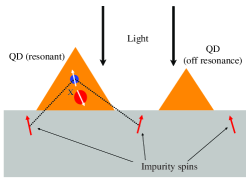
Figure 1: Scheme the system: localized spins located near self assembled QDs are coupled by an exciton created by a laser pulse. Dots of different size provide selective control and readout.

The exciton-spin part of the Hamiltonian can be written as

$$H_{0}=\epsilon N-2V(J^{2}-S^{2}-L^{2})$$ (1)

where $S$ is the total spin of the two impurities ($\hbar=1$) and $\epsilon$ is the energy of the exciton in the dot. The operators $N$ and $L$ are defined as $N=b^{\dagger}_{\uparrow}b_{\uparrow}+b^{\dagger}_{\downarrow}b_{\downarrow}$, $L_{x}=\frac{1}{2}(b^{\dagger}_{\downarrow}b_{\uparrow}+b^{\dagger}_{\uparrow}b_{\downarrow})$, $L_{y}=\frac{i}{2}(b^{\dagger}_{\downarrow}b_{\uparrow}-b^{\dagger}_{\uparrow}b_{\downarrow})$ and $L_{z}=\frac{1}{2}(b^{\dagger}_{\downarrow}b_{\downarrow}-b^{\dagger}_{\uparrow}b_{\uparrow})~{}.$ $b^{\dagger}_{\downarrow}$ creates an optically active exciton with electron spin $-1/2$ and hole spin $+3/2$, while $b^{\dagger}_{\uparrow}$ creates a dark state exciton with electron spin $+1/2$ and hole spin $+3/2$. The total angular momentum $J_{i}=L_{i}+S_{i}$, and $V$ is the exchange interaction between the impurity spins and the photoexcited electron in the dot. The strength and the sign of $V$ depend on the system. For instance, this coupling is expected to be ferromagnetic for electrons in the dot interacting with localized rare-earth magnetic impuritites, while it is antiferromagnetic for a dot mediating the interaction between shallow donors. piermarocchi04 ; ramon04 Without loss of generality, we will assume $V>0$ below. The coupling of the excitons in the QD and the external laser field is given by

$$H^{(LX)}=\frac{\Omega(t)}{2}e^{-i\omega t}b^{\dagger}_{\downarrow}+hc$$ (2)

where $\Omega(t)$ is the time-dependent Rabi energy associated with the optical pulses, and $\omega$ is the energy of the laser. We consider only anti-clockwise polarization ($\sigma_{+}$) which generates excitons with electron and hole spin states $-1/2$ and $+3/2$, respectively. Excitons with hole spin $-3/2$ are not included in the model since they are not excited by $\sigma_{+}$ light and the impurity spins can only flip the spin of the photoexcited electron.

A scheme of the relevant energy levels is given in Fig. 2. In the ground state $n=0$ we have the singlet and the triplet states corresponding to the two non-interacting impurities. In the excited state $n=1$, the electron in the dot splits the triplet states in a quadruplet $J=3/2$ and a doublet $J=1/2$. The total Hilbert space is thus spanned by a total of $12$ states. The arrows in the scheme identify the selection rules for $\sigma_{+}$ optical transitions. The transitions have different oscillator strengths, which are calculated using the Clebsch-Gordan coefficients. Notice that the light does not connect directly states with different spin $S$. The structure of the energy levels provides a natural readout scheme for the coded logical qubit $|0_{L}\rangle$, $|1_{L}\rangle$ in the exchange-only scheme. divincenzo00 An optical setup similar to the one for single spin readout besombes04 could be used: a single peak at $\epsilon$ corresponds to $|0_{L}\rangle$ while two peaks separated by $6V$ correspond to the logical state $|1_{L}\rangle$.

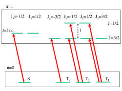
Figure 2: Energy level diagram and optical selection rules for $\sigma_{+}$ polarized light. In $n=1$, the total splitting is $j=6V$.

III quantum control

In order to illustrate how to design the optical control we consider the production of maximal spin entanglement. We choose the the initial state $|\uparrow\downarrow\rangle\otimes|0\rangle$ as the tensor product of a linear superposition of impurity states $\{|S\rangle,|T_{0}\rangle\}$, and the exciton $|0\rangle$ representing an empty QD. We consider separately the case of infinite and finite $\gamma^{-1}$, i.e. spontaneous radiative recombination lifetime for the exciton in the dot. In the first case we determine analitically the control parameters that provide maximal spin entanglement. In the second case, we solve numerically the master equation for the full system in Fig. 2. This will allow us to analyze errors due both to the radiative recombination and to the finite probability of remaining with an exciton in the dot at the end of a pulse. The latter is an error similar to a double occupancy error in the case of spins controlled by gate voltages hu00 . Ideally, the QD must be empty at the end of each optical pulse, and this can be achieved by an adiabatic evolution, or by a nonadiabatic evolution plus additional conditions in the pulse area kaplan04 .

III.1 Infinite radiative lifetime

We first analyze the ideal case of a nonadiabatic evolution at $\gamma=0$. We call nonadiabatic the evolution that follows from a laser resonant with at least one transition between the $n=0$ and $n=1$ subspaces in Fig. 2. This implies that there is a substantial exchange of energy between the electromagnetic field and the dot, which in turn results in a significant population inversion during the pulse. Using a numerical simulation we illustrate in Fig. 3 the evolution of the $|S\rangle$ and $|T_{0}\rangle$ populations under a Gaussian pulse giving a Rabi energy of the form,

$$\Omega(t)=\frac{\Omega}{\sqrt{\pi}}e^{-(t/\tau)^{2}}~{}.$$ (3)

The pulse is resonant with the bare exciton energy, which in the scheme of Fig. 2 corresponds to a resonant transition for the singlet state. In order to have no excitonic population at the end of the pulse, we need the pulse area for the resonant excitation to be multiple of $2\pi$, therefore $\Omega$ and $\tau$ are chosen so that the pulse area is $\Omega\tau=8\pi$. Notice that the population of the ground state singlet $|S\rangle$ is completely depleted during the pulse but at the end comes back to the original population ($0.5$). In contrast, the triplet ($|T_{0}\rangle$) population follows an adiabatic evolution due to the exchange interaction affecting the optical resonance. In Fig. 3 (inset) we show the real and imaginary part of the coherence $\langle S|\rho|T_{0}\rangle$. In order to create the maximally entangled state we need a $\pm\pi/2$ phase in this matrix element and the chosen optical pulse achieves this goal. This relative phase transforms, for example, the state $|\uparrow\downarrow\rangle$ into $2^{-1/2}(|S\rangle+i|T_{0}\rangle)\propto|\uparrow\downarrow\rangle+i|\downarrow\uparrow\rangle$. For a given value of the exchange coupling $V$ and pulse width $\tau$, the maximum intensity of the field $\Omega$ in Eq. (3) is found from the roots of the equation

$$\phi_{T}(\Omega,V,\tau)\pm\pi/2=0$$ (4)

where $\phi_{T}=\int_{-\infty}^{\infty}\lambda^{0}_{T}(t)~{}dt$ is the dynamic phase that the state $|T_{0}\rangle$ picks up following the adiabatic evolution. Notice that since the pulse is a multiple of $2\pi$ the singlet will only pick up a trivial phase ($\pm 1$). $\lambda^{0}_{T}$ is the eigenvalue satisfying $\lambda^{0}_{T}(\pm\infty)=0$ for a 3-level Hamiltonian representing the triplet states,

$$H_{T}(t)=\frac{1}{2}\left[\begin{array}[]{ccc}0&\sqrt{\frac{2}{3}}\Omega(t)&\sqrt{\frac{1}{3}}\Omega(t)\\ \sqrt{\frac{2}{3}}\Omega(t)&2\delta-\frac{2}{3}j&0\\ \sqrt{\frac{1}{3}}\Omega(t)&0&2\delta+\frac{4}{3}j\end{array}\right]~{}.$$ (5)

The optical detuning $\delta=\epsilon-\omega$ and $j=6V$ is the splitting in the excited state between $J=3/2$ and $J=1/2$ states. If we assume that the three eigenvalues of the matrix in Eq. 5 do not cross during the pulse evolution, the expression for $\lambda^{0}_{T}(t)$ can be written as

$$\lambda^{0}_{T}(t)=\frac{j}{9}+\frac{2}{3}\delta+\frac{q(t)}{3}\cos\left(\frac{\theta(t)}{3}\right)$$ (6)

where

$$\theta(t)=2k\pi+\arccos\left(\frac{r(t)}{q^{3}(t)}\right)$$ (7)

with

$$q(t) = \sqrt{28j^{2}+12j\delta+36\delta^{2}+27\Omega^{2}(t)}$$

$$r(t) = 4(4j-3\delta)(5j+3\delta)(j+6\delta)-81(2j+3\delta)\Omega^{2}(t)~{}.$$

If the exciton impurity coupling is ferromagnetic ($j>0$), we have to take in Eq. (7) $k=1$ for $\delta>j/3$, $k=2$ for $-2j/3<\delta<j/3$, and $k=3$ for $\delta<-2j/3$. In contrast, for $j<0$, we have to take in Eq. (7) $k=1$ for $\delta>-2j/3$, $k=2$ for $1/3j<\delta<-2j/3$, and $k=3$ for $\delta<j/3$. The analytical expression in Eq. (6) allows us to determine exactly the control parameters from the roots of Eq. (4) .

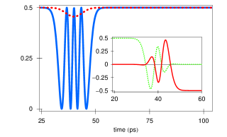
Figure 3: (Color online) Nonadiabatic control, $\gamma=0$. Evolution of the $|S\rangle$ (solid blue line) and $|T_{0}\rangle$ (dashed red line) populations under a Gaussian pulse of area $8\pi$. The temporal width of the pulse $\tau$ is $7.02$ ps and the ratio $\Omega/V$ is 0.6697. (Inset) Real (dashed green line) and imaginary (solid red line) part of the coherence $\langle S|\rho|T_{0}\rangle$.

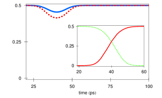
Figure 4: (Color online) Adiabatic control, $\gamma=0$. The laser is tuned in $2$ meV below the bare excitonic energy. Evolution of the $|S\rangle$ (solid blue line) and $|T_{0}\rangle$ (dashed red line) populations under a Gaussian pulse. The temporal width of the pulse $\tau$ is $10.2$ ps and the ratio $\Omega/V$ is 1.24. (Inset) Real (dashed green line) and imaginary (solid red line) part of the coherence $\langle S|\rho|T_{0}\rangle$.

In the $\gamma=0$ adiabatic regime the laser pulse is tuned away from the optical resonances between the $n=0$ and $n=1$ levels. An example of a simulation of an adiabatic control is shown in Fig. 4. The laser is tuned $2$ meV below the bare excitonic energy and $1$ meV below the triplet resonances corresponding to $J=3/2$ in Fig. 2. We plot in Fig. 4 the same quantities of Fig. 3. Notice that in this case the pulse area can be arbitrary, provided the adiabaticity is preserved. The change of phase in the coherence $\langle S|\rho|T_{0}\rangle$ is now obtained with a smooth transition. The control parameters in this adiabatic case are determined by the roots of

$$\phi_{T}(\Omega,V,\tau)-\phi_{S}(\Omega,V,\tau)\pm\pi/2=0~{}.$$ (8)

In contrast to the case of Fig. 3, the singlet now picks up a nontrivial dynamic phase $\phi_{S}=\int_{-\infty}^{\infty}\lambda^{0}_{S}(t)~{}dt~{}$ where $\lambda^{0}_{S}$ is the eigenvalue of the singlet Hamiltonian

$$H_{S}(t)=\frac{1}{2}\left[\begin{array}[]{cc}0&\Omega(t)\\ \Omega(t)&2\delta\end{array}\right]$$ (9)

with the property $\lambda^{0}_{S}(\pm\infty)=0$. As for $H_{T}$ this has a simple analytical form $\lambda^{0}_{S}(t)=\frac{\delta}{2}\pm\frac{1}{2}\sqrt{\delta^{2}+\Omega^{2}(t)}~{}$, ($+$ for $\delta<0$ and $-$ for $\delta>0$ ) which can be used to determine the control parameters from the roots of Eq. (8).

III.2 Finite radiative lifetime

In order to determine how this control scheme is affected by the finite lifetime of the exciton in the dot we introduce a finite value for $\gamma$, and solve the master equation $\dot{\rho}=-i[H,\rho]+\cal{L}[\rho]$ using the values of the control parameters corresponding to the evolution of Figs. 3 and 4. $\cal{L}[\rho]$ is the Liouvillian superoperator that can be written as ${\cal{L}}[\rho]=L^{\dagger}\rho L+\frac{1}{2}\{L^{\dagger}L,\rho\}$ where $L^{\dagger}=\sqrt{\gamma}~{}b_{\downarrow}$ accounts for the spontaneous radiative recombination of the exciton in the dot. Once $\rho$ is obtained, a $4\times 4$ reduced density matrix for the impurity spins $\rho_{S}$ is computed by tracing out the exciton degrees of freedom. The entanglement in the Bell state is mostly sensitive to decoherence processes and its analysis provides a good test for the scheme. We quantify the error on the reduced density matrix $\rho_{S}$ using two different methods, the Purity and the Peres criterion of separability. peres96 According to the Peres criterion a state is entangled iff $E_{min}<0$, where $E_{min}$ is the minimum eigenvalue of a matrix constructed by transposing the non-diagonal $2\times 2$ blocks of $\rho_{S}$. A maximally entangled state has a $E_{min}=-1/2$. The deviation from that value gives a measure of the effect of the radiative recombination on the entanglement and we quantify the entanglement error as $\Delta E=E_{min}+1/2$. The purity of $\rho_{S}$ is a different parameter that characterizes the error in the spins states due to their entanglement with the exciton in the dot. We quantify this error as $\Delta P=Tr{\rho_{S}^{2}}-1$. In principle there are errors that can disentangle the spin states without a change in the purity, for instance by affecting the phase picked up in Eq. (8). Therefore, in principle the errors induced by $\gamma$ affect independently $\Delta E$ and $\Delta P$.

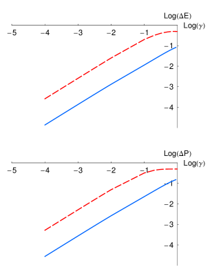
Figure 5: (Color online) Log-Log plot of the deviation from maximal entanglement (upper panel) and maximal purity (lower panel) as a function of the radiative recombination $\gamma$ (in meV). Solid blue line: adiabatic evolution. Dashed red line: nonadiabatic evolution.

We compare in Fig. 5 the errors in the Entanglement $\Delta E$ (upper) and in the Purity $\Delta P$ as a function of $\gamma$ for both the adiabatic and nonadiabatic evolution. Both errors increase linearly at small $\gamma$. However, the errors in the adiabatic case are always smaller than in the nonadiabatic case in the range of parameters we have investigated. We remark that, due to the incommensurability of the eigenvalues of $H_{S}$ and $H_{T}$, there are not special conditions that would give perfect entanglement with square pulses as in the case of a direct spin-spin coupling. kaplan04 An important figure of merit for the application of this quantum control technique to quantum computation is provided by the error per gate parameter. This has to be below a threshold value in order to make scalable quantum computing possible. The estimate for such a threshold depends on assumptions on the error model and device capabilities but the $10^{-4}$ value  gottesman97 is usually used as a benchmark in typical experimental implementations. The error in the entanglement production gives an estimation of the error per gate since the quantum operation done corresponds to a $\sqrt{SWAP}$ modulo some single qubit operations. We see in Fig. 5 that the $10^{-4}$ threshold can be achieved for $\gamma$ smaller than 1$\mu eV$. Self assembled QDs have typically a ground state exciton lifetime of the order of one or more nanoseconds and would reasonably be in this region of parameters.

IV Conclusions

In conclusion, we have analyzed the entanglement production between two spin-impurities induced by an exciton in a neighboring quantum dot. In the case of $\gamma=0$, the parameters for the quantum control can be analytically determined from the roots of simple integral equations. We showed that the finite lifetime $\gamma^{-1}$ of the exciton in the dot can affect the purity of the spin states and introduces errors in the entanglement production. In addition we found that such errors increase linearly with $\gamma$ and can be kept below the $10^{-4}$ threshold for error correction if parameters typical of self assembled QDs are used in the simulation.

- (1) C. Piermarocchi and G. F. Quinteiro, Phys. Rev. B. 70, 235210 (2004).
- (2) C. Piermarocchi, P. Chen, L. J. Sham, and D. G. Steel, Phys. Rev. Lett. 89, 167402 (2002).
- (3) R. Rodriquez, A. J. Fisher, P. T. Greenland, and A. M. Stoneham, J. Phys. Condens. Matter 16, 2757 (2004).
- (4) A. M. Stoneham, A. J. Fisher, and P. T. Greenland, J. Phys. Condens. Matter 15, L447 (2003).
- (5) G. Ramon, Y. Lyanda-Geller, T. L. Reinecke and L. J. Sham, arXiv:cond-mat/0412003 (2004)
- (6) A. Nazir, B. W. Lovett, S. D. Barrett, T. P. Spiller, and G. A. D. Briggs, Phys. Rev. Lett. 93, 150502 (2004).
- (7) E. Pazy, E. Biolatti, T. Calarco, I. D’Amico, P. Zanardi, F. Rossi, and P. Zoller, Europhys. Lett. 62, 175 (2003).
- (8) P. Chen, C. Piermarocchi and L. J. Sham, Phys. Rev. Lett. 87, 067401 (2001).
- (9) J. M. Bao, A. V. Bragas, J. K. Furdyna, and R. Merlin, Nature Mat. 2, 175 (2003); J. M. Bao, A. V. Bragas, J. K. Furdyna, and R. Merlin, Solid State Commun. 127, 771 (2003); J. M. Bao, A. V. Bragas, J. K. Furdyna, and R. Merlin, Phys. Rev. B 71, 045314 (2005).
- (10) L. Besombes, Y. Léger, L. Maingault, D. Ferrand, H. Mariette, and J. Cibert, Phys. Rev. Lett. 93, 207403 (2004).
- (11) D. Bacon, J. Kempe, D. A. Lidar, and K. B. Whaley, Phys. Rev. Lett. 85, 1758 (2000).
- (12) D. P. Di Vincenzo, D. Bacon, J. Kempe, G. Burkard, and K. B. Whaley, Nature 408, 339 (2000).
- (13) Combescot and O. Betbeder-Matibet, Solid State Commun. 132, 129 (2004).
- (14) X. Hu and S. Das Sarma, Phys. Rev. A 61, 062301 (2000).
- (15) T. A. Kaplan and C. Piermarocchi, Phys. Rev. B 70, 161311(R) (2004).
- (16) A. Peres, Phys. Rev. Lett. 77, 1413 (1996).
- (17) D. Gottesman, Stabilizer Codes and Quantum Error Correction PhD thesis, Calif. Inst. Tech. Pasadena, California (1997).