Dynamics of disordered elastic systems

1 Introduction

Understanding the statics and dynamics of elastic systems in a random environment is a longstanding problem with important applications for a host of experimental systems. Such problems can be split into two broad categories: (i) propagating interfaces such as magnetic lemerle_domainwall_creep ; krusin_pinning_wall_magnet ; repain_avalanches_magnetic ; caysol_minibridge_domainwall or ferroelectric tybell_ferro_creep ; paruch_2.5 domain walls, fluid invasion in porous media wilkinson_invasion , contact line in wetting moulinet_contact_line , epitaxial growth barabasi_book or crack propagation bouchaud_crack_propagation ; (ii) periodic systems such as vortex lattices blatter_vortex_review ; nattermann_vortex_review ; giamarchi_vortex_review , charge density waves gruner_revue_cdw , or Wigner crystals of electrons andrei_wigner_2d ; giamarchi_electronic_crystals_review . In all these systems the basic physical ingredients are identical: the elastic forces tend to keep the structure ordered (flat for an interface and periodic for lattices), whereas the impurities locally promote the wandering. From the competition between disorder and elasticity emerges a complicated energy landscape with many metastable states. This results in glassy properties such as hysteresis and history dependence of the static configuration.

To study the statics, the standard tools of statistical mechanics could be applied, leading to a good understanding of the physical properties. Scaling arguments and simplified models showed that even in the limit of weak disorder, the equilibrium large scale properties of disordered elastic systems are governed by the presence of impurities. In particular, below four (internal) dimensions, displacements grow unboundedly larkin_70 with the distance, resulting in rough interfaces and loss of strict translational order in periodic structures. To go beyond simple scaling arguments and obtain a more detailed description of the system is rather difficult and requires sophisticated approaches such as replica theory mezard_variational_replica or functional renormalization group fisher_functional_rg . Much progress was recently accomplished both due to analytical and numerical advances. For interfaces, the glassy nature of the system is confirmed (so called random manifold), and a coherent picture of the system is derived from the various methods. Periodic systems have also been shown to have glassy properties but to belong to a different universality class than interfaces, with quite different behavior for the long range nature of the correlation functions giamarchi_book_young ; nattermann_vortex_review ; giamarchi_vortex_review .

The competition between disorder and elasticity manifests also in the dynamics of such systems, and if any in a more dramatic manner. Among the dynamical properties, the response of the system to an external force $F$ is specially crucial, both from a theoretical point of view, but also in connection with measurements. Indeed in most systems the velocity $v$ versus force $F$ characteristics is directly measurable and is simply linked to the transport properties (voltage-current for vortices, current-voltage for CDW and Wigner crystals, velocity-applied magnetic field for magnetic domain walls).

Some of the questions related to this issue are shown in Fig. 1.

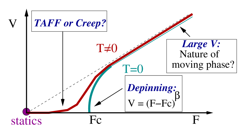
Figure 1: The velocity $v$ induced by an external force $F$ of a disordered elastic system. At zero temperature $T=0$ the system stays pinned until a critical force $F_{c}$ is reached. At finite temperature a motion can occur even for forces below threshold $F<F_{c}$ since the barriers to motion can always be passed by thermal activation.

In the presence of disorder it is natural to expect that, at zero temperature, the system remains pinned and only polarizes under the action of a small applied force, i.e. moves until it locks on a local minimum of the tilted energy landscape. At larger drive, the system follows the force $F$ and acquires a non-zero asymptotic velocity $v$. So a first set of questions is prompted by the zero temperature properties. What is $F_{c}$ ? An estimate of $F_{c}$ can be obtained via scaling arguments larkin_ovchinnikov_pinning or with a criterion for the breakdown of the large velocity expansion schmidt_hauger ; larkin_largev and related to static quantities such as the Larkin-Ovchinikov length, or computed numerically by an exact algorithm rosso_depinning_simulation . The $v-F$ curve at $T=0$ is reminiscent of the one of an order parameter in a second order phase transition fisher_depinning_meanfield . Here the system is out of equilibrium so no direct analogy is possible but this suggests that one could expect $v\sim(F-F_{c})^{\beta}$ with a dynamical critical exponent $\beta$ duemmer_depinning . Calculation of such exponents is of course an important question nattermann_stepanow_depinning ; narayan_fisher_depinning ; chauve_creep_long ; rosso_hartmann .

Another important set of questions pertain to the nature of the moving phase itself, and in particular to the behavior at large velocity: how much this moving system resembles or not the static one koshelev_dynamics ; giamarchi_moving_prl ; kolton_mglass_phases ? This concerns both the positional order properties and the fluctuations in velocity such as the ones measured in noise experiments.

Finally, one of the most important questions, and the one on which we will concentrate in these notes, is the response well below threshold $F\ll F_{c}$ at finite temperature. In this regime, the system is expected to move through thermal activation. What is the nature of this motion and what is the velocity? The simplest answer would be that the system can overcome barriers via thermal activation, anderson_kim leading to a linear response at small force of the form $v\sim e^{-U_{b}/T}F$, where $U_{b}$ is some typical barrier. However it was realized that such a typical barrier does not exist in a glassy system nattermann_rfield_rbond ; ioffe_creep ; nattermann_creep_domainwall ; feigelman_collective and that the response of the system was more complicated. The motion is actually dominated by barriers which diverge as the drive $F$ goes to zero, and thus the flow formula with finite barriers is incorrect. Well below $F_{c}$, the barriers are very high and thus the motion, usually called “creep” is extremely slow. Scaling arguments, relying on strong assumptions such as the scaling of energy barriers and the use of statics properties to describe an out of equilibrium system, were used to infer the small $F$ response. This led to a non linear response, characteristic of the creep regime, of the form $v\sim\exp(-C\,F^{-\mu}/T)$.

Given the phenomenological aspect of these predictions and the uncontrolled nature of the assumptions made, many open questions remain to be answered, in particular whether such a behavior is indeed correct kolton_string_creep and can be derived directly from microscopic equation of the motion chauve_creep_short ; chauve_creep_long . We will review these questions in these notes. The plan of the notes is as follows. In Sec. 2 we recall the basic concepts of interfaces in the presence of disorder. In Sec. 3, we recall the phenomenological derivation of the creep law. We present the microscopic derivation of the creep law from the equations of motion in Sec. 4, and discuss the similarities and differences with the phenomenological result. In Sec. 5 we focus on the situation of domain walls. Such a situation is a particularly important both for experimental realizations of the creep but also because one dimension is the extreme case for such systems. Conclusions can be found in Sec. 6.

2 Basic concepts

Let us introduce in this section the basic ingredients of the systems under study. We will focus in these short notes to the case of interfaces, but similar concepts apply to periodic systems as well. The interface is a sheet of dimension $d$ living in a space of dimensions $D$. For realistic interfaces $D=d+1$ but generalization are of course possible (for example $D=d$ corresponds to periodic systems). We call $r$ the internal coordinate of the interface and $z$ all its transverse directions. The interface position is labelled by a displacement $u(r)$ from a flat configuration. This determines totally the shape of the interface provided that $u$ is univalued, i.e. that there are no overhangs or bubbles. The case of a one dimensional interface ($d=1$) in a two dimensional film is shown in Fig. 2.

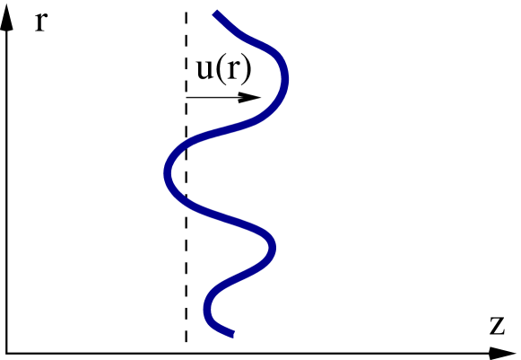
Figure 2: A one dimensional interface (domain wall) living in a two dimensional space (film). The position of the interface is determined (provided there are no overhangs or bubbles) by the displacement $u$ from a flat configuration.

Since the interface distortions cost elastic energy, its zero temperature equilibrium configuration in the absence of disorder is the flat one. Deviation from this equilibrium position are described by an Hamiltonian $H[u]$ which is a function of the displacements $u$. For small displacements one can make the usual elastic approximation

$$H[u]=\frac{1}{2}\int\frac{d^{d}q}{(2\pi)^{d}}c(q)u^{*}_{q}u_{q}$$ (1)

where $u_{q}$ is the Fourier transform of $u(r)$ and $c(q)$ are the so called elastic coefficients. If the elastic forces acting on the interface are short ranged then one has $c(q)=cq^{2}$ which corresponds to

$$H[u]=\frac{c}{2}\int d^{d}r(\nabla u(r))^{2}$$ (2)

For some interfaces where long range interactions play a role different forms for the elasticity are possible. This is in particular the case when dipolar forces nattermann_dipolar are taken into account paruch_2.5 or for the contact line in wetting joanny_contact_line and crack propagation gao_crack .

In addition to the elastic energy the interface gains some energy by coupling to the disorder. Two universality classes for the disorder exist (see Fig. 3). The so called random bond disorder corresponds to impurities that directly attract or repel the interface. On the contrary, for the so called random field disorder the pinning energy is affected by all the randomness that the interface has encountered in its previous motion. If $V(z,r)$ denotes the random potential generated by the impurities the pinning energy writes:

$$H_{\text{dis}}[u]=\int dr\begin{cases}V(u(r),r)&\text{random bond}\\ \ \int_{0}^{u(r)}dzV(z,r)&\text{random field}.\end{cases}$$ (3)

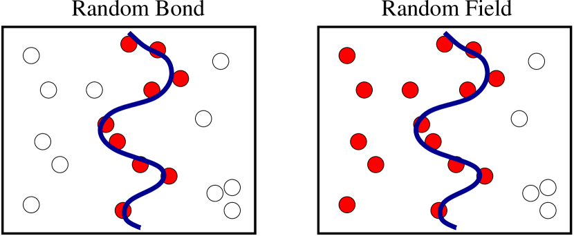
Figure 3: The two types of disorder (the names are coming from the magnetic realization of such systems). The dark circles are the impurities that contribute to the pinning energy of the interface. In the random bond case only neighboring impurities contribute while in the random filed case all the impurities on the left side of the the interface contribute. This makes the latter disorder effectively long ranged, even if the disorder potential $V(z,r)$ is short range.

The competition between disorder and elasticity manifests itself in the static properties of the interface. The presence of disorder leads to the appearance of many metastable states and glassy properties. In particular, the interface deviates from the flat configuration and becomes rough. From the scaling of the relative displacements correlation function, a roughness exponent $\zeta$ can be defined by

$$B(r)=\overline{\langle[u(r)-u(0)]^{2}\rangle}\propto r^{2\zeta}$$ (4)

where $\langle\ \ \rangle$ denotes thermodynamic average and $\overline{\cdots}$ denotes disorder average. We will not enter in more details about the statics here and refer the reader to the literature on that point kardar_growth ; barabasi_book .

Dynamics is much more complicated since the standard tools of statistical physics can not be used. One has to study the equation of motion of the system

$$\eta\frac{\partial}{\partial t}u(r,t)=-\frac{\delta H}{\delta u(r,t)}+F+\zeta(r,t)$$ (5)

This equation is written for overdamped dynamics, but can include inertia as well. $\eta$ is the friction taking into account the dissipation, $F$ the external applied force, and $\zeta(r,t)$ a thermal noise, needed to reproduce the effect of finite temperature. The correlation of the thermal noise is $\langle\zeta(r,t)\zeta(r^{\prime},t^{\prime})\rangle=2\eta T\delta(r-r^{\prime})\delta(t-t^{\prime})$. Solving this equation of motion allows to extract all the dynamical properties of the system. The presence of disorder in the Hamiltonian $H$ makes this a very complicated proposal. In the absence of the external force $F=0$, this Langevin equation allows to recover the static properties after the system has achieved its thermal equilibrium.

3 Creep, phenomenology

Let us focus here on the response of the system to a very small external force. For usual systems we expect the response to be linear. Indeed earlier theories of such a motion found a linear response. The idea is to consider that a blob of pinned material has to move in an energy landscape with characteristic barriers $U_{b}$ as shown in Fig. 4.

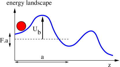
Figure 4: In the Thermally Assisted Flux Flow (TAFF) anderson_kim a region of pinned material is considered as a particle moving in an energy landscape characterized by characteristic barriers $U_{b}$. This leads to an exponentionally small but linear response.

The external force $F$ tilts the energy landscape making forward motion possible. The barriers are overcomed by thermal activation (hence the name: Thermally Assisted Flux Flow) with an Arrhenius law. If the minima are separated by a distance $a$ the velocity is

$$v\propto e^{-\beta(U_{b}-Fa/2)}-e^{-\beta(U_{b}+Fa/2)}\simeq e^{-\beta U_{b}}F$$ (6)

The response is thus linear, but exponentially small.

However this argument is grossly inadequate for a glassy system. The reason is easy to understand if one remembers that the static system is in a vitreous state. In such states a characteristic barrier $U_{b}$ does not exist, since barriers are expected to diverge as one gets closer to the ground state of the system. The TAFF formula is thus valid in systems where the glassy aspect is somehow killed and the barriers do saturate. This could be the case for example for a finite size interface. When the glassy nature of the system persists up to arbitrarily large length scales the theory should be accommodated to take into account the divergent barriers. This can be done quantitatively within the framework of the elastic description nattermann_rfield_rbond ; ioffe_creep ; feigelman_collective ; nattermann_pinning . The basic idea rests on two quite strong but reasonable assumptions: (i) the motion is so slow that one can consider at each stage the interface as motionless and use its static description; (ii) the scaling for barriers, which is quite difficult to determine, is the same as the scaling of the minimum of energy (metastable states) that can be extracted again from the static calculation. If the displacements scale as $u\sim L^{\zeta}$ then the energy of the metastable states (see (2)) scales as

$$E(L)\sim L^{d-2+2\zeta}$$ (7)

where we use that elastic and pinning energy scale the same way. Since the motion is very slow, the effect of the external force is just to tilt the energy landscape

$$E(L)-F\int d^{d}ru(r)\sim L^{d-2+2\zeta}-FL^{d+\zeta}$$ (8)

Thus, in order to make the motion to the next metastable state, one needs to move a piece of the pinned system of size

$$L_{\text{opt}}\sim\left(\frac{1}{F}\right)^{\frac{1}{2-\zeta}}$$ (9)

The size of the optimal nucleus able to move thus grows as the force decrease. Since the barriers to overcome grow with the size of the object, the minimum barrier to overcome (assuming that the scaling of the barriers is also given by (7))

$$U_{b}(F)\sim\left(\frac{1}{F}\right)^{\frac{d-2+2\zeta}{2-\zeta}}$$ (10)

leading to the well known creep formula for the velocity

$$v\propto\exp\left[-\beta U_{c}\left(\frac{F_{c}}{F}\right)^{\mu}\right]$$ (11)

where $F_{c}$ is the depinning force and $U_{c}$ a characteristic energy scale and the creep exponent $\mu$ is given by,

$$\mu={\frac{d-2+2\zeta}{2-\zeta}}$$ (12)

Equations (11) and (12) are quite remarkable. They relate a dynamical property to static exponents, and shows clearly the glassy nature of the system. The corresponding motion has been called creep since it is a sub-linear response. Of course the derivation given here is phenomenological, and it will be important to check by other means whether the results here hold. This will be the goals of the two next sections, where first the creep law will be derived directly from the equation of motion in $d=4-\epsilon$ dimensions, and then the creep will be examined in the important case of $d=1$ domain walls.

4 Around four dimensions

The previous phenomenological derivation of the creep formula rests on very strong hypothesis. In particular it is assumed that: (a) the motion is dominated by the typical barriers, and not by tails of distributions in the waiting times or barriers; (b) the motion is so slow that the line has the time to completely re-equilibrate between two hopping events so that one can take all exponents as the equilibrium ones. Given the phenomenological ground of these predictions and the uncontrolled nature of the assumptions made, both for the creep and for the depinning, it is important to derive this behavior in a systematic way, directly from the equation of motion.

In principle one has simply to solve the equation of motion (5). In practice this is of course quite complicated. A natural framework for computing perturbation theory in off-equilibrium systems is the dynamical formalism janssen_dynamics_action ; martin_siggia_rose . Integrating on all configurations $u$ we can exponentiate the equation of motion by introducing an auxiliary field $\hat{u}$ :

$$\int{\cal D}u\;\delta\left(\eta\frac{\partial u}{\partial t}+\frac{\delta H}{\delta u(r,t)}-F-\zeta(r,t)\right)=\\ \int{\cal D}u{\cal D}\hat{u}\;\exp\left[i\hat{u}(\eta\frac{\partial u}{\partial t}+\frac{\delta H}{\delta u(r,t)}-F-\zeta(r,t))\right]$$ (13)

the thermal and disorder average can easily be done, leading to a field theory with some action $S$

$$S(u,\hat{u})=\int_{rt}i\hat{u}_{rt}(\eta\partial_{t}-c\nabla^{2})u_{rt}-\eta T\int_{rt}i\hat{u}_{rt}i\hat{u}_{rt}-F\int_{rt}i\hat{u}_{rt}\\ -\frac{1}{2}\int_{rtt^{\prime}}i\hat{u}_{rt}i\hat{u}_{rt^{\prime}}\Delta(u_{rt}-u_{rt^{\prime}})$$ (14)

where $\Delta$ is defined in the correlator of the pinning force $F_{p}=-\delta H_{\text{dis}}/\delta u$, as

$$\overline{F_{p}(u,r)F_{p}(u^{\prime},r^{\prime})}=\Delta(u-u^{\prime})\delta(r-r^{\prime}).$$ (15)

The functional form of this correlator depends on whether one has random bond or random field disorder (see e.g. chauve_creep_long for more details). Essentially $\Delta$ is a function with a width of the order of the correlation of the disorder along the $z$ direction. The advantages of this representation are many: disorder and thermal averages $\overline{\langle A[u]\rangle}=\langle A[u]\rangle_{S}$ of any observable $A[u]$ can be computed with the weight $e^{-S}$; the response functions to an external perturbation $h_{rt}$ are simply given by correlations with the response field: $\langle A[u]i\hat{u}_{rt}\rangle=\frac{\delta}{\delta h_{rt}}\langle A[u]\rangle$. In addition, since we are much more familiar with fields theories than with equations of motion, we have at our disposal a variety of tools to tackle the action $S$.

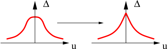
Figure 5: Although the correlator of the disorder is initially an analytic function, a non analyticity (cusp) appears at a finite scale $l_{c}$. This length scale corresponds to the Larkin-Ovchinikov length at which pinning and metastability occur.

Although it is impossible to solve the action exactly it is possible to look at its properties using a renormalization group procedure. We will not detail the procedure but just recall here the resulting functional renormalization group (FRG) flow equations chauve_creep_short ; chauve_creep_long to give a flavor of their physics

$$\partial\tilde{\Delta}(u)=(\epsilon-2\zeta)\tilde{\Delta}(u)+\zeta u\tilde{\Delta}^{\prime}(u)+\tilde{T}\tilde{\Delta}^{\prime\prime}(u)$$ (16)

$$+\int_{s>0,s^{\prime}>0}\!\!\!\!\!\!\!\!\!\!\!\!\!\!\!\!\!\!\!\!e^{-s-s^{\prime}}\left[\tilde{\Delta}^{\prime\prime}(u)\left(\tilde{\Delta}((s^{\prime}-s)\lambda)-\tilde{\Delta}(u+(s^{\prime}-s)\lambda)\right)\right.$$

$$-\tilde{\Delta}^{\prime}(u-s^{\prime}\lambda)\tilde{\Delta}^{\prime}(u+s\lambda)$$

$$\left.+\tilde{\Delta}^{\prime}((s^{\prime}+s)\lambda)\left(\tilde{\Delta}^{\prime}(u-s^{\prime}\lambda)-\tilde{\Delta}^{\prime}(u+s\lambda)\right)\right]$$

$$\partial\ln\lambda=2-\zeta-\int_{s>0}e^{-s}s\tilde{\Delta}^{\prime\prime}(s\lambda)$$

$$\partial\ln\tilde{T}=\epsilon-2-2\zeta+\int_{s>0}e^{-s}s\lambda\tilde{\Delta}^{\prime\prime\prime}(s\lambda)$$

$$\partial\tilde{F}=e^{-(2-\zeta)l}c\Lambda_{0}^{2}\int_{s>0}e^{-s}\tilde{\Delta}^{\prime}(s\lambda)$$

where $\epsilon=4-d$, $\partial$ denotes $\frac{\partial}{\partial l}$ and $\lambda=\eta_{l}v$. The tilde denotes rescaled quantities (see chauve_creep_long for the notations). Contrarily to the standard case of critical phenomena, where the potential $\Delta$ can be expanded in powers of the field and only the first terms are relevant, here all the powers of the expansion have the same dimension. It is thus necessary to renormalize the whole function fisher_frg_1 (in other words one has an infinite set of coupled renormalization equations). One of the most important consequences is shown in Fig. 5: the renormalized function $\Delta$ becomes nonanalytic beyond a certain length scale, and develop a cusp which signals pinning and the glassy properties of the system. This cusp appears at a finite length scale corresponding to the Larkin-Ovchinikov length larkin_largev and it is directly related to the existence of the finite critical force $F_{c}$ nattermann_stepanow_depinning ; narayan_fisher_depinning at zero temperature. The FRG procedure has been push up to two loop expansion 2loop ; wiese_frg_review .

The presence of a finite temperature and a finite velocity (proportional to $\lambda$) prevents the appearance of the cusp chauve_creep_short ; chauve_creep_long . For very small external force, the way the cusp is cut occurs in two steps, as shown in Fig. 6.

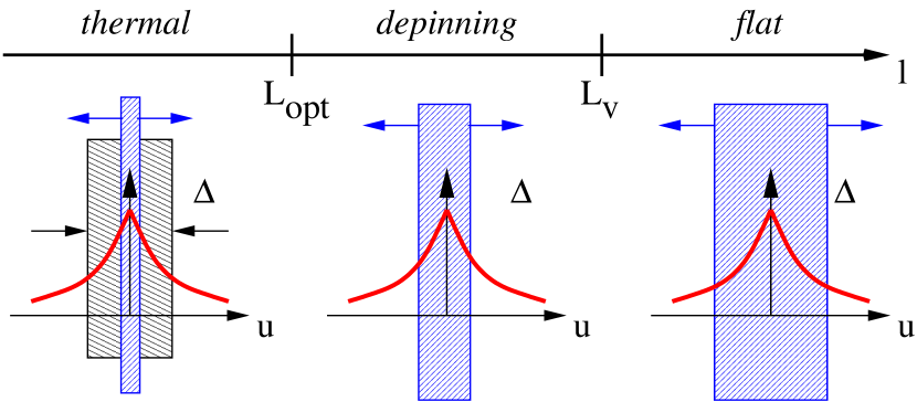
Figure 6: The cusp is rounded by both the temperature and the finite velocity of the interface. In the thermal regime, the main source of rounding comes from the temperature and the role of velocity is negligible. Then the system enters a regime in which the main source of rounding is the velocity and the role of temperature is negligible. This regime is very similar to a depinning regime. Finally the velocity rounds the whole correlator of the disorder and thus disorder is washed out by the averaging due to motion. At this length scale one recovers a purely thermal interface.

At very low velocity the cusp is cut first by the temperature and the velocity can be forgotten. A physical way to interpret this regime is that the motion consists essentially in overcoming the barriers by thermal activation. This regime corresponds essentially to the one in the phenomenological derivation of the creep. Increasing the scale $l$ the temperature renormalizes down and the velocity renormalizes up. For this reason, above a lengthscale that can be identified with $L_{\text{opt}}$, the cusp starts to be regularized by the velocity. The temperature can now be forgotten and a regime very similar to the standard depinning regime at $T=0$ takes place. Then, finally, at a certain length scale $L_{v}$ the whole $u$ dependence of the correlator of the disorder $\Delta(u)$ is erased by the finite velocity. This corresponds to a regime where the motion of the interface has averaged over the disorder and thus, in the moving frame, the interface is now simply submitted to the thermal-like noise nattermann_stepanow_depinning .

The FRG calculation of the velocity confirms the phenomenological arguments and finds the creep law (11). Moreover, at the first order in $\epsilon$, the creep exponent $\mu$ agrees with the scaling (12). The velocity behavior is thus dominated by the first (thermal) regime. On the other hand because the second regime exists, we expect that the phenomenological derivation is incorrect as far as the characteristic lengthscales of the problem are concerned. Indeed, the phenomenological derivation would predict that the characteristic size of a moving domain is the optimal length scale $L_{\text{opt}}$, which coincides with the end of the thermal regime. However the FRG equations predict that the size of a moving domain corresponds to $L_{v}$, the scale of the end of the depinning regime. A physical way to understand this behavior is to say that the motion of the thermal nucleus, of size $L_{\text{opt}}$, triggers an avalanche of a larger size $L_{v}$. The FRG thus predicts much larger avalanche scales than what should be naively expected from the phenomenological theory, as shown in Fig. 7.

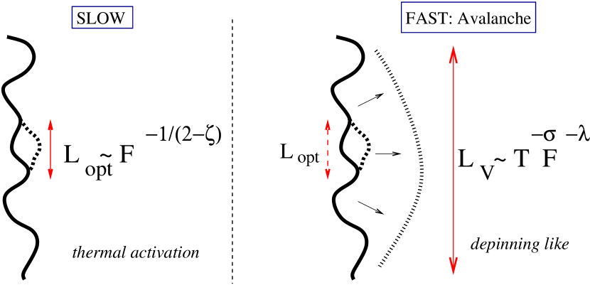
Figure 7: The phenomenological theory of creep (left) would predict that the avalanche size corresponds to the size of the thermal nucleus $L_{\text{opt}}$. From the FRG a quite different size emerges corresponding to a larger avalanche of size $L_{v}$ triggered by the thermal motion, in a way similar than for a depinning process. $\lambda$ and $\sigma$ are two characteristic exponents.

Such large avalanches are in agreement with recent experiments in magnetic systems repain_avalanches_magnetic .

Confirming the stretched exponential behavior of the creep is of course an experimental challenge given the large span of velocities needed. The first unambiguous determination of the creep law with a precise determination of the exponent was made in magnetic films, for one dimensional domain walls lemerle_domainwall_creep , and confirmed with subsequent measurements repain_avalanches_magnetic ; caysol_minibridge_domainwall . Ferroelectric systems tybell_ferro_creep ; paruch_2.5 have shown a creep exponent compatible with two dimensional domain walls in presence of dipolar forces . In periodic systems, such as vortices, it is more delicate to determine the precise value of the exponent, even when non linear behavior has been clearly observed. The experiment fuchs_creep_bglass shows a creep exponent in agreement with the theoretical predictions.

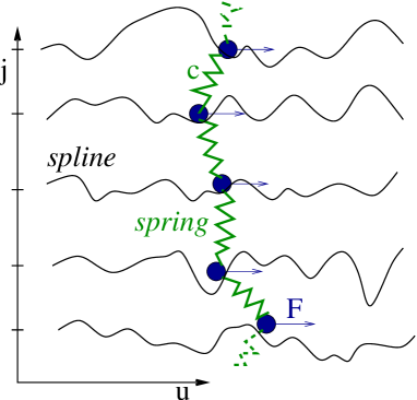
Figure 8: Discretization scheme for the elastic line driven in a random potential.

5 Low dimensional situation: domain walls

Around four dimensions the creep hypothesis gives a velocity dependence consistent with the one obtained from the microscopic derivation, at least up to the order $\epsilon$ at which the renormalization group analysis can be performed. Let us now focus at the other extreme limit, namely when the wall is one dimensional and moves in a two dimensional space. The interest in such a situation is twofold. First, as already mentioned, controlled experiments are performed on domain wall motion. Second, from the theoretical point of view the situations of a low dimensional domain wall is very interesting. Thermal effects are increasingly important as the dimension is lowered. For $d\leq 2$ they lead to a roughening of the domain wall, even in the absence of disorder (with an exponent $\zeta_{T}=(2-d)/2$). One can thus expect more intricate competition between temperature and disorder effects.

Numerical simulations are a valuable alternative theoretical tool to address this open issue. In this respect, Langevin dynamics simulations have been used to study both the velocity-force ($v$-$F)$ characteristics and the dynamic roughness $\zeta$ of an elastic string in a random potential kaper_creep_simulation ; chen_marchetti ; kolton_string_creep . In kolton_string_creep we have studied equation (5) with a short range elasticity:

$$\eta\frac{\partial}{\partial t}u(r,t)=c\partial_{r}^{2}u(r,t)+F_{p}(u,r)+F+\zeta(r,t)$$ (17)

where $F_{p}(u,r)=-\partial_{u}V(u(r),r)$ is the pinning force derived from the random bond disorder $V(u,r)$.

To solve numerically (17) we discretize the string along the $r$ direction, $r\rightarrow j=0,\ldots,L-1$, keeping $u_{j}(t)$ as a continuous variable. A second order stochastic Runge-Kutta method greenside_runge_kutta is used to integrate the resulting equations. To model a continuous random potential we generate, for each $j$, a cubic spline $V(u_{j},j)$ passing through regularly spaced uncorrelated Gaussian random points rosso_depinning_simulation . The geometry of our system is shown in Fig. 8. We are interested in the $v$-$F$ characteristics. Typical curves, obtained in the simulations, are shown in Fig. 9.

Figure 9: After kolton_string_creep . $v$-$F$ characteristics for several temperatures, increasing from bottom to top. Solid lines are fits of the creep formula (11) with $U_{c}$ and $\mu$ as fitting parameters. The inset assures the validity of the creep formula in the range of temperature and velocity analyzed.

In the whole range of temperature and pinning strength analyzed we find that the $v$-$F$ curve can be well fitted by the creep formula (11) with $U_{c}$ and $\mu$ as fitting parameters. We thus confirm the predicted stretched exponential behavior. However, contrarily to the naive creep relation (12) we find that not only $U_{c}$, but also $\mu$, depend on temperature. Since the phenomenological theory assumes that $\mu$ can be computed directly from the roughness exponent $\zeta$ it is important to study the geometrical properties of the driven string. For this reason we introduce the averaged structure factor,

$$S(q)\sim\overline{\biggl{\langle}\biggl{|}\int dru(r,t)e^{-iqr}\biggr{|}^{2}\biggr{\rangle}}.$$ (18)

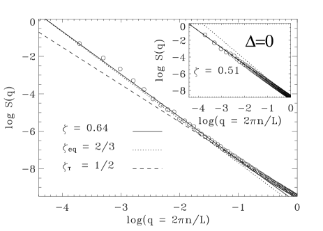
Figure 10: Structure factor $S(q)$ of the elastic line for the statics. In the presence of disorder the long distance behavior is characterized by a roughness exponent $\zeta_{eq}=2/3$, while in the absence of disorder (see inset) thermal fluctuation gives $\zeta_{T}=1/2$.

The dimensional analysis of this double integral allow us to compute $\zeta$ from $S(q)\sim q^{-(1+2\zeta)}$, valid for small $q$. In Fig. 10 we show the structure factor of an elastic string thermally equilibrated at $F=0$. We can observe a crossover between a short distance regime where thermal fluctuations are dominant ($\zeta\sim\zeta_{T}=1/2$) and a long distance disorder dominated regime where we find the well known roughness exponent $\zeta\sim\zeta_{eq}=2/3$ kardar_exponent_line .

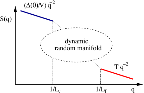
Figure 11: Sketch of $S(q)$ expected for a driven elastic line.

For the dynamics (see Fig. 11), when $F\neq 0$ one can predict that the short distance behavior $L<L_{T}$ of the elastic string is still dominated by thermal fluctuations ($\zeta_{T}=1/2$). Note that this thermally dominated regime has nothing to do with the regime derived in the previous section and valid up to the scale $L_{\text{opt}}$. In this regime disorder is already dominant and barriers are overcomed by thermal activation. On the other hand, as already discussed, the finite velocity makes the quenched disorder to act as a thermal noise at the largest length scale $l>L_{v}$. Thus, in this case, the expected exponent is also $\zeta_{v}=1/2$ nattermann_stepanow_depinning . Finally, at intermediate length scales, the physics is determined by the competition between disorder and elasticity and characterized by a non trivial random manifold roughness exponent.

A systematic analysis of the $v$-$F$ characteristics and $S(q)$ show essentially two different regimes of creep motion. In Fig. 12(a) and (b) we show the structure factor for the two cases.

Figure 12: After kolton_string_creep . Structure factor $S(q)$ of the elastic line in the driven case. Two regimes are distinguished. (a) In the low disorder/high temperature regime the roughness exponent is consistent with $\zeta_{eq}=2/3$. (b) In the high disorder/low temperature regime the roughness exponent is clearly bigger than $\zeta_{eq}$.

As predicted, we get $\zeta\sim\zeta_{T}=1/2$ for large $q$. At a certain scale we observe a crossover between the thermal and the random manifold scaling. The location of this crossover decreases as temperature (disorder) is increased (decreased). We can also observe that the second velocity-controlled crossover is not achieved in our finite-size simulation due to the very slow dynamics. Interestingly, for the small disorder case (Fig. 12(a)) the random manifold scaling gives $\zeta=0.67\pm 0.05$, in excellent agreement with the equilibrium value $\zeta_{eq}=2/3$, while a much higher roughness exponent $\zeta=0.9\pm 0.05$ is found for the strong disorder case (Fig. 12(b)). The analysis of the $v$-$F$ characteristics brings us to the same conclusion: the value of the exponent $\mu$ is close to the equilibrium value $\mu=1/4$ for low disorder (high temperature) and departs from this value when the disorder (temperature) increases (decreases). In Fig. 13 we summarize all the results.

Figure 13: After kolton_string_creep . Roughness exponent, $\zeta(T)$, and creep exponent, $\mu(T)$, vs $T$. The dashed line gives the equilibrium roughness exponent $\zeta_{eq}=2/3$, and the dotted line the purely thermal roughness $\zeta_{T}=1/2$. The expected value for the creep exponent $\mu=1/4$ is also indicated.

We notice that although the values of $\zeta$ and $\mu$ depart from the equilibrium values, the relation (12) seems still to hold, within the error bars for the two exponents. This is highly non-trivial since equation (12) is derived from a calculation of the barriers in an equilibrium situation.

We thus have found two regimes of creep motion. The first one occurs when the temperature is larger than the strength of the disorder, giving $\mu\sim 1/4$ and $\zeta\sim 2/3$ as predicted by assuming a quasi-equilibrium nucleation picture of the creep motion. This implies that the domain wall has time to re-equilibrate between hops, being the underlying assumption behind (12) essentially satisfied. The second regime occurs for temperatures smaller than the strength of the disorder, and is characterized by anomalously large values of both exponents. This clearly shows that in this regime the domain wall stays out of equilibrium, and that the naive creep hypothesis does not apply. Note that the measured roughness exponent is intermediate between the equilibrium value and the depinning value $\zeta_{dep}=1.26\pm 0.01$ rosso_depinning_simulation . The fact that the thermal nucleation which is the limiting process in the creep velocity, is in fact followed by depinning like avalanches was noted in the FRG study of the creep chauve_creep_long . Whether such avalanches and the time it would take them to relax to equilibrium is at the root of the observed increase of the exponent, is clearly an interesting but quite complicated open question.

6 Conclusions and open questions

In these short notes we have presented a brief review of the dynamical properties of interfaces in a disordered environment. We have in particular focused on the response of such interfaces to a very small external force, and the corresponding very slow motion it entails (so called creep). Clearly many important questions remain to be understood for this problem. for large dimensions the microscopic derivation clearly supports the phenomenological one as far as the velocity is concerned, but also shows that different length scales enter to describe the dynamics. In particular, it predicts a much larger avalanche size than initially anticipated. For one dimensional walls the situation is even more complex, and the very hypothesis that the wall is constantly in equilibrium between two creep processes seems incorrect at least when the disorder is not weak enough or if the temperature becomes too low. The deviations such effect might entail on the creep exponent is of course important in connection with the experimental work.

Of course these questions are only the tip of the iceberg and more subtle questions such as how such a domain wall can age in the presence of the disorder are still largely not understood, and more analytical, numerical or experimental work is clearly needed to address these issues.

7 Acknowledgments

We have benefitted from invaluable discussions with many colleagues, too numerous to thank them all here. We would however like to specially thank D. Domínguez, J. Ferré, J. P. Jamet, W. Krauth, S. Lemerle, P. Paruch, V. Repain, J.M. Triscone. TG acknowledges the many fruitful and enjoyable collaborations with P. Le Doussal and P. Chauve. This work was supported in part by the Swiss National Science Foundation under Division II.

References

- (1) S. Lemerle et al., Phys. Rev. Lett. 80, 849 (1998).
- (2) L. Krusin-Elbaum et al., Nature 410, 444 (2001).
- (3) V. Repain et al., Europhys. Lett. 68, 460 (2004).
- (4) F. Caysoll et al., Phys. Rev. Lett. 92, 107202 (2004).
- (5) T. Tybell, P. Paruch, T. Giamarchi, and J. M. Triscone, Phys. Rev. Lett. 89, 097601 (2002).
- (6) P. Paruch, J. M. Triscone, and T. Giamarchi, 2004, cond-mat/0412470.
- (7) D. Wilkinsion and J. F. Willemsen, J. Phys. A 16, 3365 (1983).
- (8) S. Moulinet, C. Guthmann, and E. Rolley, Eur. Phys. J. E 8, 437 (2002).
- (9) A.-L. Barabasi and H. E. Stanley, in Fractal Concepts in Surface Growth (Cambridge University Press, Cambridge, 1995).
- (10) E. Bouchaud et al., Journal of the Mechanics and Physics of Solids 50, 1703 (2002).
- (11) G. Blatter et al., Rev. Mod. Phys. 66, 1125 (1994).
- (12) T. Nattermann and S. Scheidl, Adv. Phys. 49, 607 (2000).
- (13) T. Giamarchi and S. Bhattacharya, in High Magnetic Fields: Applications in Condensed Matter Physics and Spectroscopy, edited by C. Berthier et al. (Springer-Verlag, Berlin, 2002), p. 314, cond-mat/0111052.
- (14) G. Grüner, Rev. Mod. Phys. 60, 1129 (1988).
- (15) E. Y. Andrei et al., Phys. Rev. Lett. 60, 2765 (1988).
- (16) T. Giamarchi, in Quantum phenomena in mesoscopic systems, edited by Italian Physical Society (IOS Press, Bologna, 2004), cond-mat/0403531.
- (17) A. I. Larkin, Sov. Phys. JETP 31, 784 (1970).
- (18) M. Mézard and G. Parisi, J. Phys. I France 1, 809 (1991).
- (19) D. S. Fisher, Phys. Rev. Lett. 56, 1964 (1986).
- (20) T. Giamarchi and P. Le Doussal, in Spin Glasses and Random fields, edited by A. P. Young (World Scientific, Singapore, 1998), p. 321, cond-mat/9705096.
- (21) A. I. Larkin and Y. N. Ovchinnikov, J. Low Temp. Phys 34, 409 (1979).
- (22) A. Schmidt and W. Hauger, J. Low Temp. Phys 11, 667 (1973).
- (23) A. I. Larkin and Y. N. Ovchinnikov, Sov. Phys. JETP 38, 854 (1974).
- (24) A. Rosso and W. Krauth, Phys. Rev. E 65, 025101R (2002).
- (25) D. S. Fisher, Phys. Rev. B 31, 1396 (1985).
- (26) O. Duemmer and W. Krauth, 2005, cond-mat/0501467.
- (27) T. Nattermann, S. Stepanow, L. H. Tang, and H. Leschhorn, J. Phys. (Paris) 2, 1483 (1992).
- (28) O. Narayan and D. Fisher, Phys. Rev. B 48, 7030 (1993).
- (29) P. Chauve, T. Giamarchi, and P. Le Doussal, Phys. Rev. B 62, 6241 (2000).
- (30) A. Rosso, A. K. Hartmann, and W. Krauth, Phys. Rev. E 67, 021602 (2003).
- (31) A. E. Koshelev and V. M. Vinokur, Phys. Rev. Lett. 73, 3580 (1994).
- (32) T. Giamarchi and P. Le Doussal, Phys. Rev. Lett. 76, 3408 (1996).
- (33) A. B. Kolton and D. D. N. Grønbech-Jensen, Phys. Rev. Lett. 83, 3061 (1999).
- (34) P. W. Anderson and Y. B. Kim, Rev. Mod. Phys. 36, 39 (1964).
- (35) T. Nattermann, Europhys. Lett. 4, 1241 (1987).
- (36) L. B. Ioffe and V. M. Vinokur, J. Phys. C 20, 6149 (1987).
- (37) T. Nattermann, Y. Shapir, and I. Vilfan, Phys. Rev. B 42, 8577 (1990).
- (38) M. Feigelman, V. B. Geshkenbein, A. I. Larkin, and V. Vinokur, Phys. Rev. Lett. 63, 2303 (1989).
- (39) A. B. Kolton, A. Rosso, and T. Giamarchi, Phys. Rev. Lett. 94, 047002 (2005).
- (40) P. Chauve, T. Giamarchi, and P. Le Doussal, Europhys. Lett. 44, 110 (1998).
- (41) T. Nattermann, J. Phys. C 16, 4125 (1983).
- (42) J. F. Joanny and P. G. de Gennes, J. Chem. Phys. 81, 552 (1984).
- (43) H. Gao and J. R. Rice, J. Appl. Mech. 56, 828 (1989).
- (44) M. Kardar, Physica B 221, 60 (1996).
- (45) T. Nattermann, Phys. Rev. Lett. 64, 2454 (1990).
- (46) H. K. Janssen, Z. Phys. B 23, 377 (1976).
- (47) P. C. Martin, E. D. Siggia, and H. A. Rose, Phys. Rev. A 8, 423 (1973).
- (48) D. S. Fisher, Phys. Rev. B 31, 7233 (1985).
- (49) P. Le Doussal, K. J. Wiese, and P. Chauve, Phys. Rev. B 66, 174201 (2002).
- (50) K. J. Wiese, Acta Physica Slovaca 52, 341 (2002), cond-mat/0205116.
- (51) D. T. Fuchs et al., Phys. Rev. Lett. 80, 4971 (1998).
- (52) H. G. Kaper et al., Phys. Rev. Lett. 71, 3713 (1993).
- (53) L. W. Chen and M. C. Marchetti, Phys. Rev. B 51, 6296 (1995).
- (54) H. S. Greenside and E. Helfand, Bell Syst. Tech. J. 60, 1927 (1981).
- (55) M. Kardar, Phys. Rev. Lett. 55, 2923 (1985).