Slow energy relaxation of macromolecules and nano-clusters in solution

Abstract

Many systems in the realm of nanophysics from both the living and inorganic world display slow relaxation kinetics of energy fluctuations. In this paper we propose a general explanation for such phenomenon, based on the effects of interactions with the solvent. Within a simple harmonic model of the system fluctuations, we demonstrate that the inhomogeneity of coupling to the solvent of the bulk and surface atoms suffices to generate a complex spectrum of decay rates. We show for Myoglobin and for a metal nano-cluster that the result is a complex, non-exponential relaxation dynamics.

Matter from both the living and the inorganic worlds displays unusual structural and dynamical properties when it is reduced to small objects of nano-metric scale  nanoworld . One interesting feature that has recently been arousing interest is the relaxation to thermal equilibrium of local or distributed temperature fluctuations. Heat dissipation experiments in metallic nano-clusters in solution have revealed that the approach to equilibrium follows a stretched-exponential law slow.clus . Similarly, experiments on proteins have shown that their relaxation after excitation may also be highly non–exponential frauenfelder ; slow.prot .

Slow energy relaxation is naturally associated with the presence of a hierarchy of relaxation times. Nevertheless, the origin of such hierarchy is not always easy to pinpoint. A common assumption is that multiple time scales arise because of the roughness of the energy landscape, i.e. lots of local minima of different depths whose sequence en route to equilibrium determines a cascade of decay times. However, while such a picture would be compatible with our current understanding of protein folding dynamics dill , such mechanism is unlikely to apply to metallic nano-clusters, which are regular stacks of identical atoms, and whose energy landscape close to the ground state is likely to be mostlyfeatureless. Yet, the relaxation dynamics in solution of proteins and nano-clusters share enough similarities to raise the question whether a common mechanism could be at work in a broad class of nano-systems.

The physiological environment of proteins is a viscous aqueous solution, while metallic nano-clusters are believed to be promising markers to study the behavior of cells and living tissues, so that an aqueous solution is also the environment in many of their applications. In this paper we propose that a natural, simple and unifying explanation for the spectrum of decay times for nano-particles in solution can be found in the different coupling to the solvent of surface and bulk atoms.

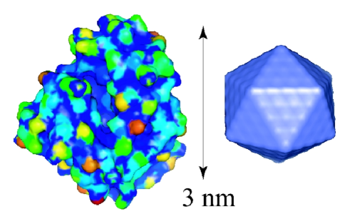
Figure 1: Structure of Myoglobin (pdb code 1A6M) and of a model icosahedral metal cluster with $N=309$ atoms. The protein structure is color–coded according to the fraction of surface accessible to the solvent at each site – from blue (low accessibility) to red (highest exposure).

The idea is that energy is dissipated to the environment only by surface atoms, whereas bulk atoms only exchange energy with each other with very little or no dissipation. To investigate the effects of the damping inhomogeneity, we model the systems under investigation as elastic networks. The interatomic interactions are simple harmonic potentials $V(\vec{r}_{i},\vec{r}_{j})=k_{ij}/2(|\vec{r}_{i}-\vec{r}_{j}|-|\vec{r}_{i0}-\vec{r}_{j0}|)^{2}$, where $\vec{r}_{i}$ is the position of atom $i$, $\vec{r}_{i0}$ its equilibrium position and $k_{ij}$ is the interaction stiffness between atoms $i$ and $j$. In the case of metallic nano-clusters this modelization is the usual, textbook description, which correctly predicts most of the general features of crystal vibrations Ashcroft . The application of elastic network models to proteins is more recent Tirion , since it had been customary to assume that proteins are characterized by complex energy landscapes. Yet, it has been realized that most features of the large- and medium-scale dynamics of proteins close to their native state can be successfully reproduced by simple harmonic interactions between amino-acids Bahar ; hinsen ; yhs . In these coarse-grained models $\vec{r}_{i}$ represents the position of the $\alpha$-carbon of the $i$-th amino-acid, $\vec{r}_{i0}$ its position in the native state as determined from X-ray crystallography or Nuclear Magnetic Resonance, and $k_{ij}$ can take different functional forms, such as $k_{ij}=k\;\theta(|\vec{r}_{i0}-\vec{r}_{j0}|-r_{c})$ or $k_{ij}=k\;\exp(-|\vec{r}_{i0}-\vec{r}_{j0}|^{2}/r_{c}^{2})$, where $r_{c}$ is a suitable cutoff (or typical) interaction distance that tunes the overall connectivity of the structure, and $k$ a phenomenological strength constant.

Treating the systems as elastic networks is indeed the simplest hypothesis. Yet, recent rigorous findings about energy relaxation in one and two dimensions suggest that even linear distributed systems display highly non-trivial relaxation properties Piazza1 ; Piazza2 . We thus start up illustrating the solution to the following problem: a chain of $N$ equal masses connected by springs of equal strength, coupled to a heat bath at its edges. The chain has free ends and at $t=0$ is at equilibrium at a temperature $T_{\scriptscriptstyle 0}$. Modeling the system à la Langevin, only the first and last particles are damped and subject to randomly fluctuating forces due to their interaction with the solvent, according to the equations

$$m\ddot{x_{i}} = k(x_{i-1}-2x_{i}+x_{i+1})\;\;\;\;i=2,...,N-1$$

$$m\ddot{x_{1}} = k(x_{2}-x_{1})-\gamma\dot{x_{1}}+\eta_{1}$$

$$m\ddot{x_{N}} = k(x_{N-1}-x_{N})-\gamma\dot{x_{N}}+\eta_{N}$$ (1)

where $\gamma$ is the viscous friction coefficient and $\eta_{k}(t)$ ($k=1,N$) is a Gaussian, delta-correlated white noise, whose standard deviation is fixed by the fluctuation dissipation theorem. We want to study the system relaxation to a temperature $T<T_{\scriptscriptstyle 0}$.

The time behavior of the system only depends on the temperature difference $\Delta T=T_{\scriptscriptstyle 0}-T$ because of the absence of local energy barriers in the energy landscape. This property shall be proved rigorously later on in the framework of the Fokker–Planck (FP) approach. As a consequence, we may solve the problem as that of a deterministic dissipative system of energy $Nk_{\scriptscriptstyle B}\Delta T$ damped at its edges. Such problem is amenable to a perturbative treatment in the limits of small and large damping, resulting in a decay spectrum of the linear modes given by Piazza1

$$\gamma(\omega)=\gamma_{\scriptscriptstyle 0}\left[1-\left(\frac{\omega}{\omega_{0}}\right)^{2}\right]\,,\ \ \gamma_{\scriptscriptstyle 0}=\begin{cases}f\gamma&\gamma\ll\omega_{0}\\ \frac{\displaystyle f\omega^{2}_{0}}{\displaystyle 4\gamma}&\gamma\gg\omega_{0}\end{cases}$$ (2)

where $\gamma$ and $\omega_{0}$ are the damping strength and band–edge frequency, respectively, and $f=2/N$ is the surface fraction. The superposition of decay constants of the form (2) allows to calculate the energy relaxation analytically, revealing a crossover in the system from the initial exponential decay $\exp(-\gamma_{\scriptscriptstyle 0}t)$ (single fastest relaxing mode) to a power–law relaxation of the type $t^{-1/2}$ (integrated regime) Piazza1 . Accordingly, the solution to the original problem may be written as

$$\frac{\langle E(t)\rangle-\langle E(\infty)\rangle}{\langle E(0)\rangle-\langle E(\infty)\rangle} =\int_{0}^{\infty}g(\omega)e^{-2\gamma(\omega)t}\,d\omega=\mathcal{I}_{0}\left(\gamma_{\scriptscriptstyle 0}t\right)$$ (3)

$$\approx\begin{cases}e^{\displaystyle-\gamma_{\scriptscriptstyle 0}t}&t\ll 1/\gamma_{\scriptscriptstyle 0}\\ (2\pi\gamma_{\scriptscriptstyle 0}t)^{-1/2}&t\gg 1/\gamma_{\scriptscriptstyle 0}\end{cases}$$

where $g(\omega)$ is the density of modes and $\mathcal{I}_{0}$ is the exponentially-modified zero–order Bessel function. The same calculation may be repeated in higher dimensions, yielding

$$\frac{\langle E(t)\rangle-\langle E(\infty)\rangle}{\langle E(0)\rangle-\langle E(\infty)\rangle}=\left[\mathcal{I}_{0}\left(\gamma_{\scriptscriptstyle 0}t\right)\right]^{d}$$ (4)

where $d$ is the spatial dimension, the parameter $\gamma_{\scriptscriptstyle 0}$ still carrying the information on the linear surface fraction $f/d$. In the rest of the Letter we show that a similar crossover from an exponential to an integrated, non–exponential regime also occurs for more complex geometries and connectivities. In order to treat the general case, we numerically compute the exact solution of the FP formulation of the problem.

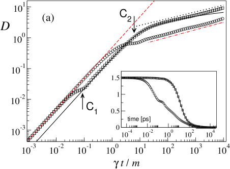
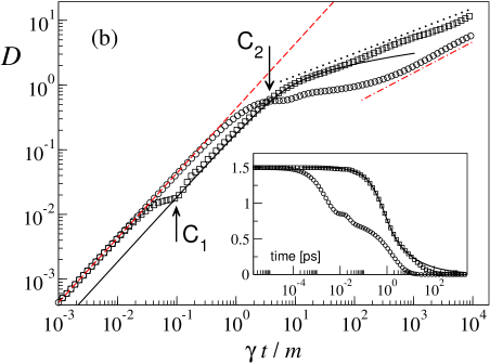
Figure 2: Relaxation to equilibrium in Myoglobin (a) and in an icosahedral cluster (b). Symbols are plots of $\mathcal{D}(t)$ (see text) as calculated through Eq. (13). Squares: under-damped regime ($\gamma/m=0.27$ ps^-1 (a) and $\gamma/m=4.27$ ps^-1 (b)). Circles: over-damped regime ($\gamma=27$ ps^-1 (a) $\gamma=427$ ps^-1 (b)). The dashed lines are plots of the straight lines $\mathcal{D}(t)=2f_{\rm eff}\gamma t$. The dotted and dot-dashed lines are stretched exponential laws with exponent $\sigma\approx 0.22$ and $\sigma\approx 0.24$, respectively (a) and $\sigma\approx 0.35$ and $\sigma\approx 0.48$, respectively (b). The solid lines are plots of formula (4) with $\gamma_{\scriptscriptstyle 0}=(f_{\rm eff}/d_{\rm eff})\gamma$ and effective dimension $d_{\rm eff}\approx 1.45$ (a), and $d_{\rm eff}\approx 0.83$ (b). In the insets we plot $\langle E(t)\rangle-\langle E(\infty)\rangle$ in units of $k_{\scriptscriptstyle B}T$ (symbols). The solid lines are the same as in the main panels. Parameters are $T_{0}=2T$, $N=194$, $f_{\rm eff}=0.242$, $r_{c}=8$ Å (a) and $N=309$, $f_{\rm eff}=0.217$, $r_{c}=6$ Å (b).

In the harmonic approximation, the total potential energy of a system of size $N$ can be written as a quadratic form

$${U}=\frac{1}{2}(X-X^{\scriptscriptstyle 0})^{T}K\,(X-X^{\scriptscriptstyle 0})$$ (5)

where $X=\{r_{1,x},r_{1,y},r_{1,z},\dots,r_{N,x},r_{N,y},r_{N,z}\}$, $X^{0}$ the same vector at equilibrium and the “contact” matrix $K$ is simply the Hessian of the potential energy function evaluated at the equilibrium structure (for the sake of simplicity, we have set all masses equal to one). Accordingly, the FP equation for the probability distribution in phase space takes the form FP

$$\frac{\partial P(Y,t|Y(0))}{\partial t}=\\ \sum_{i,j=1}^{6N}\left[-\mathbb{A}_{i,j}\frac{\partial}{\partial Y_{i}}Y_{j}+\mathbb{B}_{i,j}\frac{\partial^{2}}{\partial Y_{i}\partial Y_{j}}\right]P(Y,t|Y(0))$$ (6)

where $Y=(X-X^{\scriptscriptstyle 0},\dot{X})$ is the $6N$–dimensional vector of displacements and velocities, and the matrices $\mathbb{A}$ and $\mathbb{B}$ are given by

$$\mathbb{A}=\left(\BMAT(e)[2pt,1cm,1cm]{c.c}{c.c}0&\mathbb{I}_{\scriptscriptstyle 3N}\\ -K-\Gamma\right)\ \ \ \ \ \ \mathbb{B}=k_{\scriptscriptstyle B}T\left(\BMAT(e)[2pt,1.2cm,1.2cm]{c.c}{c.c}0&0\\ 0\Gamma\right)\quad.$$ (7)

The information on the coupling to the solvent of individual atoms is contained in the diagonal matrix $\Gamma$. The latter has the form $\Gamma_{ij}=\gamma\delta_{ij}S_{i}$, where the vector $S$ fixes the fraction of surface exposed to the solvent by each particle ($0<S_{i}<1$, $i=1,2,\dots,N$). The parameter $\gamma$ specifies the overall strength of the viscous force.

The solution of Eq. (6) is the multivariate Gaussian distribution Risken

$$P(Y,t|Y(0))=(2\pi)^{-3N}|\det C(t)|^{-1/2}\times\\ \exp\left\{-\frac{1}{2}[Y-G(t)Y(0)]^{T}C^{-1}(t)[Y-G(t)Y(0)]\right\}$$ (8)

where $C_{i,j}(t)=\langle Y_{i}(t)Y_{j}(t)\rangle$ is the block correlation matrix

$$C=\left(\BMAT(e)[2pt,1.1cm,1.1cm]{c.c}{c.c}C_{XX}&C_{X\dot{X}}\\ C_{X\dot{X}}C_{\dot{X}\dot{X}}\right)$$ (9)

and $G(t)$ is the propagator matrix. The latter can be evaluated at any time in terms of a normalized bi-orthogonal set of left and right eigenvectors of the matrix $\mathbb{A}$ (sometimes referred to as Langevin modes) as

$$G(t)=\Psi_{R}e^{\Lambda t}\Psi^{T}_{L}$$ (10)

where $\Lambda$ is the diagonal matrix of the eigenvalues of $\mathbb{A}$, and $\Psi_{R}$ and $\Psi_{L}$ are the matrices of right and left eigenvectors, respectively. It is easy to show that the evolution law for the correlations reads, in matrix form,

$$C(t)=C(\infty)+G(t)[C(0)-C(\infty)]G^{T}(t)$$ (11)

where we have introduced the equilibrium correlation matrix

$$C(\infty)=k_{\scriptscriptstyle B}T\left(\BMAT(e)[2pt,1cm,1cm]{c.c}{c.c}K^{-1}&0\\ 0\mathbb{I}_{\scriptscriptstyle 3N}\right)$$ (12)

$K^{-1}$ being the generalized inverse of matrix $K$.

In order to calculate the energy relaxation to equilibrium, we first diagonalize matrix $\mathbb{A}$ and then evaluate the correlation matrix (11) as a function of time with the aid of Eq. (10). The expression for the total energy then finally reads

$$\langle E(t)\rangle=\frac{1}{2}{\rm Tr}\,\left[C_{\dot{X}\dot{X}}(t)+KC_{XX}(t)\right]\quad.$$ (13)

To illustrate our analysis, let us examine the relaxation to equilibrium of a typical globular protein, Myoglobin, and of a model Au nano-cluster with icosahedral symmetry Siber (see Fig. 1). We estimate the effective fraction of surface exposed to the solvent at each site (the vector $S$) through standard solvent-accessible surface areas. As initial conditions, we set the specific potential energy at its equilibrium value $3/2k_{\scriptscriptstyle B}T$, while each particle is given the kinetic energy $3/2k_{\scriptscriptstyle B}T_{\scriptscriptstyle 0}$ ($T_{\scriptscriptstyle 0}>T$). This amounts to taking in Eq. (11) $C_{XX}(0)=C_{XX}(\infty)=k_{\scriptscriptstyle B}TK^{-1}$, $C_{X\dot{X}}(0)=C_{X\dot{X}}(\infty)=0$, and $C_{\dot{X}\dot{X}}(0)=k_{\scriptscriptstyle B}T_{0}\mathbb{I}_{\scriptscriptstyle 3N}$. Incidentally, the latter assignments, together with Eq. (11), also prove that the relaxation process only depends on the difference $\Delta T=T_{\scriptscriptstyle 0}-T$.

Our results are summarized in Figs. 2 (a) and (b), where we plot the quantity $\mathcal{D}(t)$ defined as

$$\mathcal{D}(t)=-\log\left[\frac{\langle E(t)\rangle-\langle E(\infty)\rangle}{\langle E(0)\rangle-\langle E(\infty)\rangle}\right]\quad.$$ (14)

This representation is most useful in identifying crossovers from an exponential law (straight line) to a slower decay regime, such as a stretched exponential of the form $\exp[-(t/\tau)^{\sigma}]$ (power law $t^{\sigma}$ with $\sigma<1$).

Remarkably, the two systems under scrutiny display the same complex behavior of the energy decay. Initially, the relaxation is exponential, which is the first signature of the linear damping on surface atoms. Accordingly, $\mathcal{D}(t)=2f_{\rm eff}\gamma t/m$, where $f_{\rm eff}=\sum_{i}S_{i}/N$ is the total effective surface fraction of the system. The first crossover occurs in correspondence with the onset of energy transfer from kinetic to potential (arrows marked C₁ in the plots), which occurs on a time scale of the order of the inverse of the maximum frequency. This crossover is independent of the damping rate $\gamma$. At this stage the potential energies of all modes have been transferred a fraction of the initial kinetic energy, and thus the relaxation process can be described in terms of Eq. (4). In fact, it turns out that the decay curves in the under-damped regime can be extremely well approximated by formula (4) with $\gamma_{\scriptscriptstyle 0}=(f_{\rm eff}/d_{\rm eff})\gamma$, where the linear surface fraction is naturally obtained by allowing for an effective dimension $d_{\rm eff}$ (see insets in Figs. 2 (a) and (b)). One-parameter fits of the exact solutions yield $d_{\rm eff}\approx 1.45$ and $d_{\rm eff}\approx 0.83$ for Myoglobin and the nano-cluster, respectively, which agree with the sizeable surface fraction of the systems.

In accordance with the prescription of formula (4), at a time of the order $d_{\rm eff}/f_{\rm eff}(\gamma/m)$ the systems undergo a second crossover to an integrated regime, which reflects the superposition of the time scales of all Langevin modes (arrows marked C₂ in the figures). This second crossover is by all means captured by the transition from exponential to a power law implicit in formula (4). In the over-damped case, the fast damping of the surface atoms increases the time scale for the dissipation of the bulk energy. As a consequence, the first stage of surface relaxation stretches until the system reaches the crossover to the integrated regime, thus merging the two crossovers.

In our chosen time span, the long-term behavior of the decay curves is best approximated by a stretched exponential (see again Figs. 2). To this concern, it is however important to stress that asymptotically the decay laws shall eventually bend again to a pure exponential. This is a finite-size effect that reflects the progressive depletion of modes, until only the slowest one is left with significant energy. Consequently, its decay constant $\gamma_{\scriptscriptstyle N}$ sets the time scale for the last exponential stage $\exp(-2\gamma_{\scriptscriptstyle N}t)$, which in both systems is of the order of $10^{5}$ in natural time units ($\omega_{0}=2$). This effect may make it hard to distinguish between a stretched exponential and a slow transition from power-law to exponential.

In this Letter we have shown that the inhomogeneity of coupling to the solvent of the surface and core atoms naturally produces a hierarchy of relaxation times, and hence complex energy relaxation, in systems as un-suspect as harmonic bead-spring networks. It can be argued that non-linear effects could also affect the nature of relaxation dynamics straub . However, within our treatment, at least for small polynomial non-linearities, an-harmonic effects are not expected to introduce dramatic modifications. In fact, the fast damping of low-frequency modes with respect to band-edge ones rapidly hinders effective inter-mode energy exchange. This phenomenon has been well documented in one- and two-dimensional lattices with quartic anharmonicity Piazza1 ; Piazza2 , where the crossover from exponential to a collective, power-law regime has been observed during relaxation irrespective of the anharmonicity strength. It is however interesting to recall that relaxation in non-linear systems is under certain circumstances associated with spontaneous energy localization Piazza1 ; Aubry1 . This phenomenon is definitely worth attention for example in the context of protein dynamics, as it may play a role in relaxation and redistribution of local energy fluctuations, such as after hydrolysis of ATP molecules.

We stress that our results are qualitatively consistent with a number of experimental observations slow.clus ; slow.prot . However, further experimental work would be necessary in order to discriminate between our model and alternative explanations, such as ruggedness of the system energy landscape frauenfelder .

The authors wish to thank A. Siber for providing the coordinate file of the nano-cluster and A. Pasquarello for a critical reading of the manuscript.

References

- (1) E. Tosatti and S. Prestipino, Science, 289 (5479), 561 (2000).
- (2) M. Hu and G. V. Hartland, J. Phys. Chem. B, 106, 7029 (2002).
- (3) H. Frauenfelder, F. Parak and R.D. Young Ann. Rev. Bioph. Bioph. Chem., 17, 451 (1988).
- (4) A. Xie, L. Van Der Meer and R. H. Austin, J. Biol. Phys., 28, 147 (2002).
- (5) K. A. Dill and H. S. Chan, Nat. Struct. Biol., 4, 10 (1997).
- (6) see e.g. N. W. Ashcroft and N. D. Mermin, Solid State Physics, Holt, Rinehart and Winston, New York (1976).
- (7) M. M. Tirion, Phys. Rev. Lett. 77, 1905 (1996).
- (8) T. Haliloglu, I. Bahar and B. Erman, Phys. Rev. Lett., 79, 3090 (1997); A. R. Atligan, S. R. Durrell, R. L. Jernigan, M. C. Demirel, O. Keskin and I. Bahar, Biophys. J., 80, 505 (2001).
- (9) K. Hinsen, Proteins, 33, 417 (1998).
- (10) F. Tama and Y. H. Sanejouand, Protein Engineering, 14, 1 (2001).
- (11) F. Piazza, S. Lepri and R. Livi, J. Phys. A, 34, 9803 (2001).
- (12) F. Piazza, S. Lepri and R. Livi, Chaos, 13, 2 (2003).
- (13) M. C. Wang and G. E. Uhlenbeck, Rev. Mod. Phys. 17, 323 (1945).
- (14) H. Risken, The Fokker–Planck Equation, Springer, New York (1984).
- (15) A. Siber, Phys. Rev. B 70, 075407 (2004).
- (16) D.E. Sagnella and J.E. Straub J. Phys. Chem. B, 105, 7057 (2001).
- (17) G. P. Tsironis and S. Aubry, Phys. Rev. Lett., 77, 5225 (1996).