Criticality in quantum triangular antiferromagnets via fermionized vortices

Abstract

We revisit two-dimensional frustrated quantum magnetism from a new perspective, with the aim of exploring new critical points and critical phases. We study easy-plane triangular antiferromagnets using a dual vortex approach, fermionizing the vortices with a Chern-Simons field. Herein we develop this technique for integer-spin systems which generically exhibit a simple paramagnetic phase as well as magnetically-ordered phases with coplanar and collinear spin order. Within the fermionized-vortex approach, we derive a low-energy effective theory containing Dirac fermions with two flavors minimally coupled to a $U(1)$ and a Chern-Simons gauge field. At criticality we argue that the Chern-Simons gauge field can be subsumed into the $U(1)$ gauge field, and up to irrelevant interactions one arrives at quantum electrodynamics in (2+1) dimensions (QED3). Moreover, we conjecture that critical QED3 with full $SU(2)$ flavor symmetry describes the $O(4)$ multicritical point of the spin model where the paramagnet and two magnetically-ordered phases merge. The remarkable implication is that QED3 with flavor SU(2) symmetry is dual to ordinary critical $\Phi^{4}$ field theory with $O(4)$ symmetry. This leads to a number of unexpected, verifiable predictions for QED3. A connection of our fermionized-vortex approach with the dipole interpretation of the $\nu=1/2$ fractional quantum Hall state is also demonstrated. The approach introduced in this paper will be applied to spin-1/2 systems in a forthcoming publication.

I Introduction

Geometrically frustrated two-dimensional (2D) quantum spin systems provide promising settings for the realization of exotic quantum phenomena due to the frustration-enhanced role of quantum fluctuations. The quasi-2D spin-1/2 triangular antiferromagnet $\text{Cs}_{2}\text{CuCl}_{4}$ and the organic Mott insulator $\kappa\text{-(ET)}_{2}\text{Cu}_{2}(\text{CN})_{3}$ provide two noteworthy examples that have generated much interest. While $\text{Cs}_{2}\text{CuCl}_{4}$ exhibits “cycloid” magnetic order at low temperatures, evidence of a spin-liquid phase with deconfined spinon excitations was found at higher temperatures.Coldea et al. (2001, 2003) Moreover, application of an in-plane magnetic field suppressed magnetic order down to the lowest temperatures achieved, which might indicate a stabilization of the spin-liquid phase.Coldea et al. (2001) In the organic material $\kappa\text{-(ET)}_{2}\text{Cu}_{2}(\text{CN})_{3}$, NMR measurements show no signs of magnetic ordering, suggesting a spin-liquid phase as a candidate ground state.Shimizu et al. (2003)

Understanding critical spin-liquid states in 2D frustrated spin-1/2 systems is a central issue that has been the focus of significant theoretical attention in response to the above experiments. Several authors have attempted to access spin-liquid phases in these systems using slave-fermion and slave-boson mean field approaches,Chung et al. (2001, 2003); Zhou and Wen and recent workIsakov et al. has studied universal properties near the quantum phase transition between a spiral magnetic state and one such spin liquid with gapped bosonic spinons. Spin-liquid states were also recently examined using slave-particle mean field approaches in the triangular lattice Hubbard model near the Mott transition, which is argued to be relevant for $\kappa\text{-(ET)}_{2}\text{Cu}_{2}(\text{CN})_{3}$.Lee and Lee ; Motrunich

The purpose of this paper is to introduce a new dual vortex approach to frustrated quantum spin systems that allows one to gain insight into critical spin-liquid phases coming from the easy-plane regime. Our goal will be to illustrate how one can formulate and analyze an effective low-energy dual theory describing criticality in frustrated quantum systems using fermionized vortices. As we will see, an advantage of this approach is that critical points and critical phases arise rather naturally from this perspective.

In the present paper we develop the fermionized-vortex approach by studying easy-plane integer-spin triangular antiferromagnets, postponing an analysis of the more challenging spin-1/2 systems for a future publication. In the integer-spin case, a direct Euclidean formulation of the quantum spin model is free of Berry phases, and therefore equivalent to a classical system of stacked triangular antiferromagnets. Thus, a fairly complete analysis is accessible in the direct spin language. Generically, such systems exhibit a paramagnetic phase, a magnetically-ordered phase with collinear spin order, and the well-known coplanar $\sqrt{3}\times\sqrt{3}$ state, and much is known about the intervening phase transitions.

Using the direct analysis as a guide, we are led to a number of surprising results in the fermionized-vortex formulation, which we now summarize. We conjecture that criticality in the spin model is described by critical quantum electrodynamics in (2+1) dimensions (QED3) with two flavors of two-component Dirac fermions minimally coupled to a noncompact gauge field. In particular, we conjecture that this critical QED3 theory describes the $O(4)$ multicritical point of the spin model where the paramagnet merges with the coplanar and collinear ordered phases. In other words, we propose that critical QED3 with $SU(2)$ flavor symmetry is dual to $O(4)$ critical $\Phi^{4}$ theory. Some remarkable predictions for the former theory follow from this conjecture, and can in principle be used to test its validity. Namely, we predict that single-monopole insertions in the QED3 theory, which add discrete units of $2\pi$ gauge flux, have the same scaling dimension as the ordering field in the $O(4)$ theory. In fact, the correspondence between the two theories can be stated by observing that there are two distinct monopole insertions in the QED3, associating a complex field with each monopole, and grouping the two complex fields into an $O(4)$ vector. Furthermore, fermionic bilinears $\overline{\psi}\bm{\tau}\psi$, which are not part of any conserved current, and double-strength monopoles in QED3 are predicted to have identical scaling dimensions, equal to that of the quadratic anisotropy fields at the $O(4)$ fixed point. It would be quite remarkable if the scaling dimensions for these seemingly unrelated operators indeed merge at the QED3 fixed point.

Given the length of this paper, it will be worthwhile to now provide an overview of the fermionized-vortex approach and describe the main steps that lead to our results for the integer-spin triangular antiferromagnet. We will first illustrate how one obtains a low-energy description of fermionized vortices, and then present a more detailed summary of the integer-spin case. We will also mention below an application of this approach in a different context, namely treating bosons at filling factor $\nu=1$, which reproduces the so-called “dipole picture” of the compressible quantum Hall fluid.

We start by highlighting the difficulties associated with frustration encountered in a conventional duality approach. Frustrated easy-plane spin models are equivalent to systems of bosons hopping in a magnetic field inducing frustration, and can be readily cast into the dual vortex representation.Fisher and Lee (1989) A crucial feature of the resulting dual theory is that the vortices are at finite density due to the underlying frustration. The finite vortex density together with the strong vortex interactions present a serious obstacle in treating the bosonic vortices, as it is not clear how one can obtain a low-energy description of such degrees of freedom that describes criticality in the spin system. However, we will demonstrate that fermionizing the vortices via Chern-Simons flux attachment allows one to successfully construct a low-energy dual vortex description in both the integer-spin and spin-1/2 cases. From the view of spin systems the principal gain here is the ability to describe the latter, as a direct analysis in the spin-1/2 case is plagued by Berry phases. Nevertheless, even in the case of integer-spin systems, the dual approach leads to interesting and unexpected predictions as mentioned above.

The formulation of a low-energy dual theory proceeds schematically as follows. Let us focus on the easy-plane triangular lattice antiferromagnet (either integer-spin or spin-1/2), which dualizes to a system of half-filled bosonic vortices on the honeycomb lattice with “electromagnetic” interactions. First, the bosonic vortices are converted into fermions carrying $2\pi$ fictitious flux via a Jordan-Wigner transformationFradkin (1989). At this stage, the dual theory describes fermionic vortices hopping on the dual lattice, coupled to a Chern-Simons field and $U(1)$ gauge field that mediates logarithmic vortex interactions. Next, one considers a mean-field state in which fluctuations in the gauge fields are ignored and the flux is taken as an average background. Such “flux-smeared” treatments have been successful in the composite-particle approach to the fractional quantum Hall effect.Heinonen (1998) Pursuing a similar approach in the context of spin systems, Lopez et al.Lopez et al. (1994) developed a theory of the square-lattice Heisenberg antiferromagnet in terms of fermions coupled to a Chern-Simons field. Compared with the latter application, we have an advantage working with vortices as there is an additional $U(1)$ gauge field which gives rise to long-range interactions that strongly suppress vortex density fluctuations. This fact will play a central role in our analysis. Exchange statistics are consequently expected to play a lesser role compared with the case of weakly-interacting fermions. Replacing the Chern-Simons flux by its average should then be a good starting point for deriving a low-energy theory, and the resulting continuum theory should be more tractable.

It is straightforward to diagonalize the “flux-smeared” mean-field hopping Hamiltonian, which at vortex half-filling reveals two Dirac nodes in the integer-spin case and four Dirac nodes in the spin-1/2 case. Focusing on excitations in the vicinity of these nodes and restoring the gauge fluctuations, one finally arrives at a low-energy Dirac theory with either two or four species of fermions coupled to the Chern-Simons and $U(1)$ gauge fields. In the absence of the Chern-Simons field, the theory becomes identical to QED3.

In the spin-1/2 case, this dual theory has a very rich structure, and describes either a critical point in the spin model or a new critical spin-liquid phase. As mentioned above, we defer an analysis of spin-1/2 systems to a subsequent paper, focusing instead on the integer-spin case. Integer-spin systems provide an ideal setting for us to establish the dual approach introduced here, as much is known about their critical behavior from a direct analysis of the spin model. Viewed another way, using the known results from a direct approach leads us to the remarkable predictions described above for the dual critical theory, which are highly nontrivial from the latter perspective. We proceed now by providing a more detailed summary of the dual analysis for the integer-spin case, beginning with the spin model to make the preceding discussion more concrete.

Throughout the paper, the easy-plane spins are cast in terms of quantum rotors. The integer-spin Hamiltonian with nearest-neighbor interactions then reads

$$H_{XY}=J\sum_{\langle{\bf rr^{\prime}}\rangle}\cos(\varphi_{\bf r}-\varphi_{\bf r^{\prime}})+U\sum_{\bf r}n_{\bf r}^{2},$$ (1)

where $n_{\bf r}$ is the density, $\varphi_{\bf r}$ is the conjugate phase, and $J,U>0$. For small $U/J$ [i.e., low temperatures in the corresponding (2+1)D classical system], this model realizes the well-known $\sqrt{3}\times\sqrt{3}$ coplanar ordered phase, although deformations of the model can give rise to collinear magnetic order as well. For large $U/J$ the paramagnetic phase arises. The dual vortex Hamiltonian obtained from Eq. (1) can be conveniently written

$${\mathcal{H}}_{\text{dual}} = -2t_{v}\sum_{\langle{\bf xx^{\prime}}\rangle}\cos(\theta_{\bf x}-\theta_{\bf x^{\prime}}-a_{\bf xx^{\prime}})$$ (2)

$$+ \sum_{\bf xx^{\prime}}(N_{\bf x}-1/2)V_{\bf xx^{\prime}}(N_{\bf x^{\prime}}-1/2)$$

$$+ U^{\prime}\sum_{\bf r}(\Delta\times a)_{\bf r}^{2}+J^{\prime}\sum_{\langle{\bf xx^{\prime}}\rangle}e_{\bf xx^{\prime}}^{2},$$

with $J^{\prime},U^{\prime}>0$. Here $a_{\bf xx^{\prime}}\in{\mathbb{R}}$ is a gauge field living on the links of the dual honeycomb lattice and $e_{\bf xx^{\prime}}$ is the conjugate electric field, $e^{i\theta_{\bf x}}$ is a vortex creation operator, and $N_{\bf x}$ is the vortex number operator. $(\Delta\times a)_{\bf r}$ in the last line denotes a lattice curl around each hexagon of the dual lattice. The $t_{v}$ term allows nearest-neighbor vortex hopping, and $V_{\bf xx^{\prime}}$ encodes the logarithmic vortex interactions. This form of the dual Hamiltonian makes manifest the half-filling of the vortices.

To proceed, the vortices are converted into fermions coupled to a Chern-Simons gauge field. Because the vortices are half-filled, the Chern-Simons flux through each dual plaquette averages to $2\pi$, which on the lattice is equivalent to zero flux. Hence, in the flux-smeared mean-field state we simply set the gauge fields to zero. We emphasize again that this is expected to be a good approximation due to the vortex interactions, which strongly suppress density fluctuations. One then has fermions at half-filling hopping on the honeycomb lattice. Diagonalizing the resulting hopping Hamiltonian, one finds two Dirac nodes. These nodes occur at the same wavevectors – namely, the $\sqrt{3}\times\sqrt{3}$ ordering wavevectors – that characterize the low-energy physics in the Landau approach to the spin model, which are not apparent in the dual theory of bosonic vortices but arise naturally in the fermionized representation. A low-energy description can be obtained by focusing only on excitations near these nodes, and upon restoring gauge fluctuations one finds the following Euclidean Lagrangian density,

$${\mathcal{L}} = \overline{\psi}_{a}\gamma^{\mu}(\partial_{\mu}-ia_{\mu}-iA_{\mu})\psi_{a}$$ (3)

$$+ \frac{1}{2e^{2}}(\epsilon_{\mu\nu\lambda}\partial_{\nu}a_{\lambda})^{2}+\frac{i}{4\pi}\epsilon_{\mu\nu\lambda}A_{\mu}\partial_{\nu}A_{\lambda}+{\mathcal{L}}_{\rm 4f}.$$

Here $\psi_{R/L}$ denote the two-component spinors corresponding to each node, the flavor index $a=R/L$ is implicitly summed, and $A$ is the Chern-Simons field. The usual form for the Chern-Simons action above enforces the flux attachment that restores the bosonic exchange statistics to the vortices. Finally, ${\mathcal{L}}_{\rm 4f}$ represents four-fermion terms arising from short-range interactions allowed in the microscopic model.

The phases of the original spin model correspond to massive phases for the fermions in this formulation. The paramagnetic phase is realized in the dual fermionic language as an integer quantum Hall state, with gapped excitations corresponding to the magnon of the paramagnet. The magnetically-ordered states correspond to spontaneous mass generation driven by fermion interactions; the $\sqrt{3}\times\sqrt{3}$ spin state is obtained as a vortex “charge-ordered” state, while the collinearly-ordered states are realized as vortex valence bond solids.

Since the fermionized dual formulation faithfully captures the phases of the original spin model, it is natural to ask about the phase transitions in this framework. Our exploration of criticality begins by implementing the following trick. First, note that the fermions couple to the combination $\tilde{a}_{\mu}=a_{\mu}+A_{\mu}$. Rewriting the Lagrangian in terms of this sum field, we then integrate out the Chern-Simons field to arrive at a Lagrangian of the form

$${\mathcal{L}} = \overline{\psi}_{a}\gamma^{\mu}(\partial_{\mu}-i\tilde{a}_{\mu})\psi_{a}+\frac{1}{2e^{2}}(\epsilon_{\mu\nu\lambda}\partial_{\nu}\tilde{a}_{\lambda})^{2}$$ (4)

$$+ {\cal L}_{4f}+i\frac{\pi}{e^{4}}(\nabla\times\tilde{a})\cdot(\nabla\times\nabla\times\tilde{a})~{}.$$

Remarkably, the lowest-order term generated by this procedure is the last Chern-Simons-like term containing three derivatives, which at criticality is irrelevant by power counting compared to the Maxwell term. It is therefore tempting to drop this term altogether, which is tantamount to discarding the bosonic exchange statistics and replacing the bosonic vortices by fermions without any statistical flux attachment, or more precisely a complete ‘screening’ of the statistical gauge field. Such a replacement leads to an additional symmetry corresponding to the naïve time reversal for fermions without any Chern-Simons field, a symmetry which the higher-derivative term violates. The unimportance of exchange statistics and concomitant emergence of this additional time-reversal symmetry at criticality seems plausible on physical grounds since the logarithmic vortex interactions strongly suppress density fluctuations. Indeed, the trick performed above is only possible because of the additional $U(1)$ gauge field that mediates these interactions. We postulate that it is indeed legitimate at criticality to drop this higher-derivative term, and that the resulting QED3 theory,

$${\mathcal{L}}_{QED3}=\overline{\psi}_{a}\gamma^{\mu}(\partial_{\mu}-i\tilde{a}_{\mu})\psi_{a}+\frac{1}{2e^{2}}(\epsilon_{\mu\nu\lambda}\partial_{\nu}\tilde{a}_{\lambda})^{2}+{\cal L}_{4f},$$ (5)

contains a description of criticality in the spin model. Furthermore, we boldly conjecture that the critical QED3 theory with the full $SU(2)$ symmetry describes the $O(4)$ multicritical point of the spin model where the paramagnet and two magnetically-ordered phases meet.

We support the above conjecture by establishing the symmetry-equivalence of operators in the spin model with operators in QED3. Specifically, we identify the two complex order parameter fields of the spin model with the two leading monopole insertions of QED3, which add discrete units of $2\pi$ gauge flux. Moreover, we establish the equivalence of the various spin bilinears with fermionic bilinears and double-strength monopole operators of QED3. At the multicritical point, all of the spin bilinears (except the energy) must have the same scaling dimension due to the emergent global $O(4)$ symmetry. This leads us to another bold prediction: specific fermionic bilinears and double-strength monopole insertions in QED3 with two fermion species have the same scaling dimension. We again remark that this would be quite surprising, as from the perspective of the dual theory there is a priori no apparent relation between these operators.

The above predictions are in principle verifiable in lattice QED3 simulations.Hands et al. (2004) However, this likely requires fine-tuning of the lattice model to criticality, since we expect that the system generically ends up in a phase with spontaneously-generated mass driven by the fermion interactions that become relevant for the low number of fermion flavors in our theory. In particular, based on the correspondence with the $O(4)$ fixed point, we expect two four-fermion interactions to be relevant at the QED3 fixed point (one strongly relevant and one weakly relevant). We note that we have performed a leading-order “large-$N$” analysis to assess the stability of the QED3 fixed point in the limit of a large number of fermion flavors, where gauge fluctuations are suppressed. This analysis suggests that only one interaction in the two-flavor theory is relevant; however, higher-order corrections could certainly dominate and lead to two relevant interactions as predicted above.

We now want to give a physical view of the fermionized vortices and also point out a connection with the so-called dipole interpretation of a Fermi-liquid-like state of bosons at filling factor $\nu=1$.Pasquier and Haldane (1998); Read (1998) This system was studied in connection with the Halperin, Lee, and Read (HLR) theoryHalperin et al. (1993) of a compressible fractional quantum Hall state for electrons at $\nu=1/2$. In the direct Chern-Simons approach, the two systems lead to very similar theories, but many researchers have argued the need for improvement over the HLR treatment (for a recent review see Ref. Murthy and Shankar, 2003). A detailed picture for bosons at $\nu=1$ is developed in Refs. Read, 1998; Pasquier and Haldane, 1998 working in the lowest Landau level. The present approach of fermionizing vortices rather than the original bosons provides an alternative and perhaps more straightforward route for describing this system and obtaining the results of Ref. Read, 1998. Our approach is closest in spirit to Ref. Lee, 1998, which also uses duality to represent vortices. The fermionized vortices appear to be ‘natural’ fermionic degrees of freedom for describing the compressible quantum Hall state. We also note an early workFeigelman et al. (1993) where the qualitative possibility of fermionic vortices was raised in a context closer to frustrated easy-plane magnets.

The vortex fermionization procedure is essentially the same as for the spin model described above. More details for this case can be found in Appendix A. Dualizing the $\nu=1$ bosons, one obtains a theory of bosonic vortices at filling factor $\nu_{\rm dual}=1/\nu=1$, with mean vortex density equal to the density of the original bosons $\bar{\rho}$. Again, unlike the original bosons, the vortices interact via a 2D electromagnetic interaction, and fermionization of vortices gives a more controlled treatment. We obtain fermions in zero average field, coupled to a $U(1)$ gauge field, $a$, and a Chern-Simons gauge field, $A$. This theory is very similar to Eq. (3), but with nonrelativistic fermions at density $\bar{\rho}$. With this theory, one can, for example, reproduce the physical response properties expected of the compressible stateRead (1998) by using an RPA approximation for integrating out the fermions.

It is useful to exhibit the equivalent of Eq. (4) in the present case,

$${\mathcal{L}}_{\nu=1} = \psi^{\dagger}\left(\partial_{\tau}-\frac{[{\bm{\nabla}}-i\tilde{\bm{a}}]^{2}}{2m_{\rm vort}}\right)\psi-i\tilde{a}_{0}(\psi^{\dagger}\psi-\bar{\rho})+\dots~{}.$$ (6)

Here $m_{\rm vort}$ is a phenomenological vortex mass. As before, $\tilde{a}=a+A$, and the Chern-Simons field has been integrated out. The final action has nonrelativistic fermions coupled to the gauge field $\tilde{a}$. As detailed in Appendix A, in the lowest Landau level limit there is no Chern-Simons like term for the field $\tilde{a}$ in contrast to Eq. (4), and the theory has the same structure as in Ref. Read, 1998.

In the present formulation, the fermions are neutral and do not couple directly to external fields. However, their dynamics dictates that they carry electrical dipole moments oriented perpendicular to their momentum ${\bm{k}}$ and of strength proportional to $|{\bm{k}}|$, which can be loosely viewed as a dumbbell formed by an original boson and a vortex. This can be seen schematically as follows. First we note that the flux of $\tilde{\bm{a}}$ is equal to the difference in the boson and vortex densities:

$${\bm{\nabla}}\wedge\tilde{\bm{a}}={\bm{\nabla}}\wedge{\bm{a}}+{\bm{\nabla}}\wedge{\bm{A}}=2\pi(\rho_{\rm bos}-\rho_{\rm vort})~{}.$$ (7)

Here ${\bm{\nabla}}\wedge\tilde{\bm{a}}=\epsilon_{ij}\partial_{i}\tilde{a}_{j}$ denotes a 2d scalar curl; we also define $(\wedge{\bm{v}})_{i}=\epsilon_{ij}v_{j}$ for a 2d vector ${\bm{v}}$. Consider now a wavepacket moving with momentum ${\bm{k}}$ in the $\hat{\bf y}$ direction, and imagine a finite extent in the $\hat{\bf x}$ direction. In the region of the wavepacket, we have $\tilde{a}_{y}=|{\bm{k}}|$, while $\tilde{a}_{y}$ is zero to the left and to the right of the wavepacket. Then ${\bm{\nabla}}\wedge\tilde{\bm{a}}\sim\partial_{x}\tilde{a}_{y}$ is positive near the left edge and negative near the right edge, i.e. the boson density is higher than the vortex density on the left side of the moving fermion and vice versa on the right side. A more formal calculation is presented in Appendix A and gives the following dipolar expression for the original boson density in terms of the fermionic fields:

$$\delta\rho_{\rm bos}({\bm{q}})=i{\bm{q}}\cdot\int\frac{d^{2}k}{(2\pi)^{2}}\;\frac{\wedge{\bm{k}}}{2\pi\bar{\rho}}\;\psi^{\dagger}_{{\bm{k}}-{\bm{q}}/2}\psi_{{\bm{k}}+{\bm{q}}/2}~{}.$$ (8)

Thus, by fermionizing the vortices we indeed obtain a description of the compressible $\nu=1$ state very similar to the dipole picture, and this is achieved in a rather simple way without using the lowest Landau level projection. The success of our approach in this case makes us more confident in the application to frustrated spin systems.

The remainder of the paper focuses on the integer-spin triangular antiferromagnet and is arranged as follows. In Sec. II we review the phases and critical behavior that arise from a direct analysis of the spin model. The duality mapping is introduced in Sec. III. In Sec. IV the fermionized-vortex formulation is developed. A low-energy continuum theory is obtained here, and we also discuss how to recover the phases of the spin model from the fermionic picture. An analysis of the QED3 theory conjectured to describe criticality in the spin model is carried out in Sec. V. We conclude with a summary and discussion in Sec. VI.

II Direct Landau Theory

II.1 The Model

In this paper we focus on quantum triangular XY antiferromagnets with integer spin, described by the Hamiltonian

$$H=J/2\sum_{\langle{\bf rr^{\prime}}\rangle}(S_{\bf r}^{+}S_{\bf r^{\prime}}^{-}+S_{\bf r}^{-}S_{\bf r^{\prime}}^{+})+U\sum_{\bf r}(S_{\bf r}^{z})^{2},$$ (9)

with $J,U>0$, $S_{\bf r}^{\pm}=S_{\bf r}^{x}\pm iS_{\bf r}^{y}$, and $[S_{\bf r}^{\alpha},S_{\bf r^{\prime}}^{\beta}]=i\delta_{\bf rr^{\prime}}\epsilon_{\alpha\beta\gamma}S_{\bf r}^{\gamma}$. Rather than working with spin models, it will be particularly convenient to instead model such easy-plane systems with rotor variables, introducing an integer-valued field $n_{\bf r}$ and a $2\pi$-periodic phase variable $\varphi_{\bf r}$ that satisfy $[\varphi_{\bf r},n_{\bf r^{\prime}}]=i\delta_{\bf rr^{\prime}}$. Upon making the identification, $S_{\bf r}^{+}\to e^{i\varphi_{\bf r}}$ and $S_{\bf r}^{z}\to n_{\bf r}$, the appropriate rotor XY Hamiltonian reads,

$$H_{XY}=J\sum_{\langle{\bf rr^{\prime}}\rangle}\cos(\varphi_{\bf r}-\varphi_{\bf r^{\prime}})+U\sum_{\bf r}n_{\bf r}^{2}.$$ (10)

Equation (10) can equivalently be written

$$H_{XY}=-J\sum_{\langle{\bf rr^{\prime}}\rangle}\cos(\phi_{\bf r}-\phi_{\bf r^{\prime}}+{\cal A}^{0}_{\bf rr^{\prime}})+U\sum_{\bf r}n_{\bf r}^{2},$$ (11)

where we have introduced new phase variables $\phi_{\bf r}$ and a static vector potential ${\cal A}^{0}_{\bf rr^{\prime}}$ that induces $\pi$ flux per triangular plaquette. In this form, the nearest-neighbor couplings can be viewed as ferromagnetic, with frustration arising instead from the flux through each plaquette. The model can alternatively be viewed as bosons at integer-filling hopping on the triangular lattice in an external field giving rise to one-half flux quantum per triangular plaquette.

A closely related model also described by Eq. (11) is the fully-frustrated XY model on a square lattice, which has applications to rectangular Josephson junction arrays. The techniques applied to the triangular antiferromagnets in this paper can be extended in a straightforward manner to this case as well.

Within a Euclidean path integral representation, the 2D quantum model becomes identical to a vertical stacking of classical triangular XY antiferromagnets with ferromagnetic XY coupling between successive planes, imaginary time giving one extra classical dimension. This classical model has been extensively studied, and much is known about the phases and intervening phase transitions. We will be particularly interested in the phase transitions, which are quantum transitions in the spin model. In this section we will briefly review the known results obtained from a Landau-Ginzburg-Wilson analysis and from Monte Carlo studies. This summary of the direct approach to these models will later serve as a useful counterpart to our dual approach.

II.2 Low-energy Landau Theory

A low-energy effective theory for the triangular XY antiferromagnet can be obtained by introducing a Hubbard-Stratonovich transformation that replaces $e^{i\varphi_{i}}$ by a “soft spin” $\Phi_{i}^{*}$ with the same correlations. This leads to a Euclidean action of the form

$$S = \int_{\tau}\bigg{[}\sum_{\bf r}(|\partial_{\tau}\Phi_{\bf r}|^{2}+m|\Phi_{\bf r}|^{2}+u|\Phi_{\bf r}|^{4})$$ (12)

$$+ {\mathcal{J}}\sum_{\langle{\bf rr^{\prime}}\rangle}(\Phi_{\bf r}^{*}\Phi_{\bf r^{\prime}}+c.c.)\bigg{]},$$

with ${\mathcal{J}}>0$. [Note that we used the angle variables appearing in Eq. (10) to implement this transformation.] Diagonalizing the kinetic part of the action in momentum space, one finds two global minima at wavevectors $\pm{\bf Q}$, where ${\bf Q}=(4\pi/3,0)$. The low-energy physics can be captured by expanding the fields around these wavevectors by writing

$$\Phi({\bf r})\approx e^{i{\bf Q}\cdot{\bf r}}\Phi_{R}({\bf r})+e^{-i{\bf Q}\cdot{\bf r}}\Phi_{L}({\bf r}),$$ (13)

where $\Phi_{R/L}$ are complex fields assumed to be slowly-varying on the lattice scale.

To explore the phases of the system within a Landau-Ginzburg-Wilson framework, one needs to construct an effective action for these fields that respects the microscopic symmetries of the underlying lattice model. In particular, the action must preserve the following discrete lattice symmetries: translation by triangular lattice vectors $\delta{\bf r}$ ($T_{\delta\bf r}$), $x$-reflection [${\cal R}_{x}:(x,y)\to(-x,y)$], and $\pi/3$ rotation about a lattice site ($R_{\pi/3}$). Additionally, the action must be invariant under a number of internal symmetries, specifically a global $U(1)$ symmetry, $\varphi_{\bf r}\to\varphi_{\bf r}+\alpha$; a “particle-hole” or “charge” conjugation (${\mathcal{C}}$) symmetry,

$${\mathcal{C}}\;:\quad n_{\bf r}\rightarrow-n_{\bf r},\quad\varphi_{\bf r}\rightarrow-\varphi_{\bf r};$$ (14)

and spin time reversal ($\mathcal{T}$) which sends $S_{\bf r}^{\alpha}\rightarrow-S_{\bf r}^{\alpha}$,

$${\mathcal{T}}\;:\quad n_{\bf r}\rightarrow-n_{\bf r},\quad\varphi_{\bf r}\rightarrow\varphi_{\bf r}+\pi,\quad i\rightarrow-i.$$ (15)

Under these symmetry operations, the continuum fields $\Phi_{R/L}$ transform according to

$$T_{\delta{\bf r}} : \Phi_{R/L}\rightarrow e^{\pm i{\bf Q}\cdot{\delta{\bf r}}}\Phi_{R/L},$$

$${\cal R}_{x},R_{\pi/3} : \Phi_{R}\leftrightarrow\Phi_{L},$$

$$U(1) : \Phi_{R/L}\rightarrow e^{i\alpha}\Phi_{R/L},$$ (16)

$${\mathcal{C}} : \Phi_{R/L}\rightarrow\Phi_{L/R}^{*},$$

$${\mathcal{T}} : \Phi_{R/L}\rightarrow\Phi_{R/L}^{*}.$$

In the last line above, we followed time reversal by a $U(1)$ transformation to remove an overall minus sign.

These symmetry constraints lead to a continuum action of the form

$$S_{eff} = \int_{{\bf r},\tau}\bigg{\{}\sum_{a=R/L}(|\partial_{\mu}\Phi_{a}|^{2}+r|\Phi_{a}|^{2})$$ (17)

$$+ u_{4}(|\Phi_{R}|^{2}+|\Phi_{L}|^{2})^{2}+v_{4}|\Phi_{R}|^{2}|\Phi_{L}|^{2}$$

$$- v_{6}[(\Phi_{R}^{*}\Phi_{L})^{3}+c.c.)]\bigg{\}}.$$

The $v_{6}$ term has been included since it is the lowest-order term that reduces the symmetry down to the global $U(1)$ of the microscopic model. Note that when $v_{4}=v_{6}=0$ the action acquires an $O(4)$ symmetry. On the other hand, when $v_{6}=0$ and $v_{4}=-2u_{4}$ the action reduces to two decoupled $U(1)$ models.

We now proceed to explore the phases that arise from Eq. (17) within mean-field theory, assuming $u_{4}>0$ but allowing $r$, $v_{4}$, and $v_{6}$ to be either positive or negative.

II.3 Phases

1. The simplest phase arises when $r>0$ so that $\langle\Phi_{a}\rangle=0$. This corresponds to the quantum paramagnet with $\langle S^{-}\rangle=0$ at each site.

When $r<0$, magnetic order develops, with the character depending on the sign of $v_{4}$:

2. The case $r<0$, $v_{4}>0$ favors a state with $\langle\Phi_{R}\rangle\neq 0$ and $\langle\Phi_{L}\rangle=0$ (or vice versa). Taking $\langle\Phi_{R}\rangle=1$, the order parameter in terms of the original spin variables is $\langle S_{\bf r}^{-}\rangle=e^{i{\bf Q}\cdot{\bf r}}$. This corresponds to the $\sqrt{3}\times\sqrt{3}$ state with $120^{\circ}$ coplanar order, whose spin configuration is illustrated in Fig. 1(a).

3. When $r,v_{4}<0$, states with $\langle\Phi_{R/L}\rangle\sim e^{i\theta_{R/L}}\neq 0$ emerge. These states are characterized by collinear spin order, which can be obtained from

$$\langle S_{\bf r}^{-}\rangle\sim e^{i\theta_{+}/2}\cos({\bf Q}\cdot{\bf r}+\theta_{-}/2),$$ (18)

where $\theta_{\pm}\equiv\theta_{R}\pm\theta_{L}$. Two types of collinear spin states can occur depending on the phase difference $\theta_{-}$, which is determined by the sign of $v_{6}$. (i) For $v_{6}>0$, the action is minimized with a phase difference of $\theta_{-}=2n\pi/3$, where $n$ is an integer. The resulting spin order on the three sublattices of the triangular lattice can be written schematically as $(1,-\frac{1}{2},-\frac{1}{2})$. This can be viewed as the dice-lattice collinear antiferromagnetic state depicted in Fig. 1(b), where “happy” nearest-neighbor bonds with spins aligned antiparallel form a dice lattice as shown by the solid lines. There are three distinct such ground states (in addition to broken global $U(1)$ symmetry) corresponding to the three inequivalent values of $\theta_{-}$. (ii) When $v_{6}<0$, a phase difference of $\theta_{-}=(2n+1)\pi/3$ is preferred. The spin order on the three sublattices is then $(1,-1,0)$, which can be viewed as hexagonal collinear antiferromagnetic order as illustrated in Fig. 1(c). In this state, spins on one of the three hexagonal subnetworks of the triangular lattice order antiferromagnetically, while spins on the remaining sites fluctuate around zero average. Here also there are three distinct ground states arising from the inequivalent values of $\theta_{-}$.

One can also distinguish between the coplanar and collinear magnetic orders by considering chirality and bond energy wave operators. Spin chirality $\kappa_{p}$ at each triangular plaquette $p$ can be defined by

$$\kappa_{p}\sim\sum_{\langle{\bf rr^{\prime}}\rangle\in p}\!\!\!\!\!\!\!\!\!\!\!\!\!\circlearrowleft\>\>\sin(\varphi_{\bf r^{\prime}}-\varphi_{\bf r}),$$ (19)

where the sum is over the links of the plaquette oriented counterclockwise. A local chirality operator is obtained by summing $\kappa_{p}$ over local “up” triangles. A bond energy wave operator may be defined as

$$B_{{\bf rr}^{\prime}}\sim e^{i{\bf Q}\cdot({\bf r}+{\bf r^{\prime}})}\cos(\varphi_{\bf r}-\varphi_{\bf r^{\prime}})~{}.$$ (20)

In terms of the continuum fields $\Phi_{R/L}$, we identify

$$\kappa \sim |\Phi_{R}|^{2}-|\Phi_{L}|^{2}\equiv K_{z}~{},$$

$$B \sim \Phi_{R}^{*}\Phi_{L}\equiv(K_{x}+iK_{y})/2~{}.$$ (21)

Here we have introduced a three-component vector field,

$$\bm{K}=\Phi^{*}_{a}\bm{\tau}_{ab}\Phi_{b},$$ (22)

with $\bm{\tau}=(\tau^{x},\tau^{y},\tau^{z})$ a vector of Pauli matrices. In the coplanar phase, the vector $\bm{K}$ points in the $\pm K_{z}$ direction, while in the collinear phase it lies in the $(K_{x},K_{y})$ plane. The degeneracy in the plane is lifted by the $v_{6}$ term, leaving three possible ordering directions $\theta_{-}$ for each collinear phase as discussed above.

Figure 1: (a) Coplanar spin configuration in the $\sqrt{3}\times\sqrt{3}$ ordered state. (b) Dice-lattice collinear antiferromagnetic state. Bold lines denote satisfied bonds, which form a dice lattice, while the remaining bonds are frustrated. $|\langle S^{-}\rangle|$ is roughly twice as large on sites with long arrows than on sites with short arrows. (c) Hexagonal collinear antiferromagnetic state. Circles represent fluctuating spins with $\langle S^{-}\rangle=0$. Satisfied bonds denoted by bold lines form a hexagonal lattice.

Microscopically, the coplanar, collinear, and paramagnetic phases can be realized in the classical stacked triangular XY antiferromagnet with an additional “boson pair hopping” term,

$$H_{cl} = -J\sum_{{\bf r},z}\cos[\varphi_{{\bf r},z+1}-\varphi_{{\bf r},z}]$$ (23)

$$+ J\sum_{\langle{\bf rr^{\prime}}\rangle,z}\cos[\varphi_{{\bf r},z}-\varphi_{{\bf r^{\prime}},z}]$$

$$- J^{\prime}\sum_{\langle{\bf rr^{\prime}}\rangle,z}\cos[2(\varphi_{{\bf r},z}-\varphi_{{\bf r^{\prime}},z})],$$

where $J^{\prime}>0$ and the $z$ coordinate labels the different triangular lattice planes. The $\sqrt{3}\times\sqrt{3}$ coplanar phase is the ground state when $J^{\prime}\ll J$. As $J^{\prime}$ increases, collinear antiferromagnet order eventually becomes more energetically favorable. Of course, at high enough temperature we obtain the paramagnetic phase. A sketch of the phase diagram containing the three phases is shown in Fig. 2(a).

Figure 2: (a) Sketch of the phase diagram in the vicinity of the coplanar-collinear transition. (b) Putative renormalization group flows in the $(r,v_{4})$ plane assuming a continuous transition from both the coplanar and collinear states to the paramagnet.

II.4 Critical Behavior

Significant numerical and analytical effort has been directed towards understanding the phase transitions occurring in classical stacked triangular XY antiferromagnets. For a recent review, the reader is referred to Refs. Kawamura, 1998; Pelissetto and Vicari, 2002; Delamotte et al., 2004; Calabrese et al., 2004. Here, we shall only highlight the known results that are pertinent to the present work. A brief discussion of our own exploratory Monte Carlo study of the classical model Eq. (23) that realizes both the coplanar and collinear (hexagonal) spin-ordered phases will also be given.

In mean field theory, the paramagnet to magnetically-ordered transitions are continuous, while the transition from the coplanar to the collinear state is first order.

The transition between the paramagnet and the collinear state also appears to be continuous in our Monte Carlo study of the model Eq. (23) near the multicritical point where the three phases meet. Moreover, such a continuous transition is expected to be governed by a $U(1)\times U(1)$ fixed point with $v_{4}^{*}=-2u_{4}^{*}$ and $v_{6}^{*}=0$. Small deviations from the condition $v_{4}=-2u_{4}$ give rise to energy-energy coupling of the two $U(1)$ models, which is irrelevant at the decoupled fixed point in three dimensions.Pelissetto and Vicari (2002); Sak (1974) It should be noted that a $4-\epsilon$ expansion in the $v_{4}<0$ case predicts a continuous transition characterized by a different stable fixed point, while the $U(1)\times U(1)$ fixed point is found to be unstable in that approach.Kawamura (1988); Pelissetto and Vicari (2002) Thus in this case the $4-\epsilon$ expansion does not capture the critical physics in three dimensions.

The nature of the transition between the paramagnetic and coplanar phases is controversial.Pelissetto and Vicari (2002); Delamotte et al. (2004); Calabrese et al. (2004) Starting with Kawamura, several Monte Carlo simulations on the stacked triangular XY antiferromagnet conclude that the transition is continuous,Kawamura (1992); Plumer and Mailhot (1994); Boubcheur et al. (1996); Zukovic et al. (2002) which also appears to be the case in our Monte Carlo simulations in the vicinity of the multicritical point. However, recent simulations on larger lattices claim a very weak first-order transition,Itakura (2003); Peles et al. (2004) and simulations of modified XY systems expected to be in the same universality class have also seen a first-order transition.Loison and Schotte (1998); Peles et al. (2004) On the other hand, Ref. Calabrese et al., 2004 claims a continuous transition in the vicinity of the $O(4)$ fixed point in a model which is a lattice discretization of the action Eq. (17).

Analytical results for the paramagnet-to-coplanar transition are conflicting as well. For instance, recent six-loop perturbative renormalization group calculations in $d=3$ dimensionsPelissetto et al. (2001); Calabrese et al. (2002) find a stable “chiral” fixed point as conjectured by KawamuraKawamura (1988). On the other hand, “non-perturbative” renormalization group techniques predict a weak first-order transition.Delamotte et al. (2004) The $4-\epsilon$ expansion in the XY case ($n=2$ case in Ref. Kawamura, 1988) finds runaway flows for $v_{4}>0$, which would be interpreted as predicting a first-order transition.

Finally, the multicritical point where the three phases meet is described by an $O(4)$ fixed point with $v_{4}^{*}=v_{6}^{*}=0$; this fixed point is unstable towards introducing a small nonzero $v_{4}$ term.

Figure 2(b) contains a sketch of the renormalization group flows in the ($r,v_{4}$) plane expected if the transition from the paramagnet to the coplanar state is indeed continuous and governed by the corresponding fixed point, labeled “C”. (In the figure, the $u_{4}$ axis is perpendicular to the plane, and we are considering fixed points that are stable in this direction.) Fixed point C would disappear if this transition is first-order, leading to unstable flows toward $v_{4}\to\infty$. We note the possibility of observing crossover behavior controlled by the unstable $O(4)$ fixed point shown in Fig. 2(b) by fine-tuning both $r$ and $v_{4}$. This can be explored with Monte Carlo simulations of $H_{cl}$ by observing scaling in the vicinity of the multicritical point where the paramagnet, coplanar, and collinear phases meet in Fig. 2(a).

Table 1: Transformation properties of the bosonic fields and bilinears under the microscopic symmetries. Here $K_{\pm}=K_{x}\pm iK_{y}$ and $I_{\pm}=I_{x}\pm iI_{y}$. For brevity, the lattice coordinates which should transform appropriately under the lattice symmetries have been suppressed. We also show field transformations under the modified reflection $\tilde{\cal R}_{x}\equiv{\cal R}_{x}{\cal C}{\cal T}$, which will be useful later.

	$T_{\bf\delta r}$	$R_{\pi/3},{\mathcal{R}}_{x}$	${\mathcal{C}}$	${\mathcal{T}}$	$\tilde{\mathcal{R}}_{x}$
$\Phi_{R/L}\to$	$e^{\pm i{\bf Q}\cdot\delta{\bf r}}\Phi_{R/L}$	$\Phi_{L/R}$	$\Phi_{L/R}^{*}$	$\Phi_{R/L}^{*}$	$\Phi_{R/L}$
$K_{z}\to$	$K_{z}$	$-K_{z}$	$-K_{z}$	$K_{z}$	$K_{z}$
$K_{\pm}\to$	$e^{\mp 2i{\bf Q\cdot\delta r}}K_{\pm}$	$K_{\mp}$	$K_{\pm}$	$K_{\mp}$	$K_{\pm}$
$I_{z}\to$	$I_{z}$	$I_{z}$	$-I^{*}_{z}$	$I^{*}_{z}$	$-I_{z}$
$I_{\pm}\to$	$e^{\pm 2i{\bf Q\cdot\delta r}}I_{\pm}$	$-I_{\mp}$	$I^{*}_{\mp}$	$I^{*}_{\pm}$	$-I_{\pm}$

To examine the $O(4)$ symmetry at the multicritical point, it is convenient to express $\Phi_{R/L}$ as

$$\Phi_{R}=\chi_{1}+i\chi_{2},\quad\Phi_{L}=\chi_{3}+i\chi_{4},$$ (24)

where $\chi_{j}$ are real fields. One expects that $\vec{\chi}\equiv(\chi_{1},\chi_{2},\chi_{3},\chi_{4})$ should transform as an $O(4)$ vector, and the ten independent bilinears $\chi_{i}\chi_{j}$ can be decomposed into an $O(4)$ scalar,

$$K_{0}\equiv\Phi_{a}^{*}\Phi_{a}=\vec{\chi}^{2}~{},$$ (25)

and a traceless, symmetric $4\times 4$ matrix that transforms as a second rank tensor representation of $O(4)$. It will be useful later to observe that these nine bilinears can be arranged into the $SU(2)$ vector $\bm{K}$ defined in Eq. (22), together with two other $SU(2)$ vectors:

$$\bm{I}=\Phi_{a}[\bm{\tau}\tau^{y}]_{ab}\Phi_{b},$$ (26)

and its Hermitian conjugate, $\bm{I}^{*}$. Under the global $U(1)$ symmetry one has $\bm{K}\to\bm{K}$ and $\bm{I}\to e^{2i\alpha}\bm{I}$. For future comparisons the transformation properties of these nine bilinears under the remaining microscopic symmetries are shown in Table 1. The $O(4)$ scalar $K_{0}$ defined in Eq. (25) is invariant under all of the above microscopic symmetries.

One can furnish explicit microscopic realizations of the bilinears $\bm{I}$ and $\bm{I}^{*}$, just as we did in Eq. (21) for the bilinears $\bm{K}$. In our Monte Carlo study of the model Eq. (23), we monitored the apparent scaling dimensions of the nine bilinears and find that these indeed merge upon approaching the multicritical point, consistent with the expectation for the $O(4)$ fixed point.

III Dual Vortex Theory

III.1 Duality Mapping

In this section we introduce the dual formalism that will be used throughout the remainder of the paper. At this point, it will prove convenient to work with the Hamiltonian as written in Eq. (11), where frustration arises from the flux induced by the vector potential ${\mathcal{A}^{0}_{\bf rr^{\prime}}}$. We will implement the standard XY duality,Fisher and Lee (1989) expressing the Hamiltonian in terms of gauge fields living on the links of the dual lattice, which in the case of the triangular lattice is the honeycomb (see Fig. 3).

As a first step, we define oriented gauge fields $\tilde{e}_{\bf xx^{\prime}}\in[-1/2,1/2)$ and $a_{\bf xx^{\prime}}\in 2\pi{\mathbb{Z}}$ living on the links of the honeycomb lattice, where ${\bf x}$ and ${\bf x^{\prime}}$ label nearest-neighbor dual lattice sites. (We reserve “${\bf x}$” and “${\bf r}$” for sites of the honeycomb and triangular lattices, respectively.) The dual “electric field” $\tilde{e}_{\bf xx^{\prime}}$ and “vector potential” $a_{\bf xx^{\prime}}$ satisfy the commutation relation $[\tilde{e}_{\bf xx^{\prime}},a_{\bf xx^{\prime}}]=i$ on the same link and commute on different links.

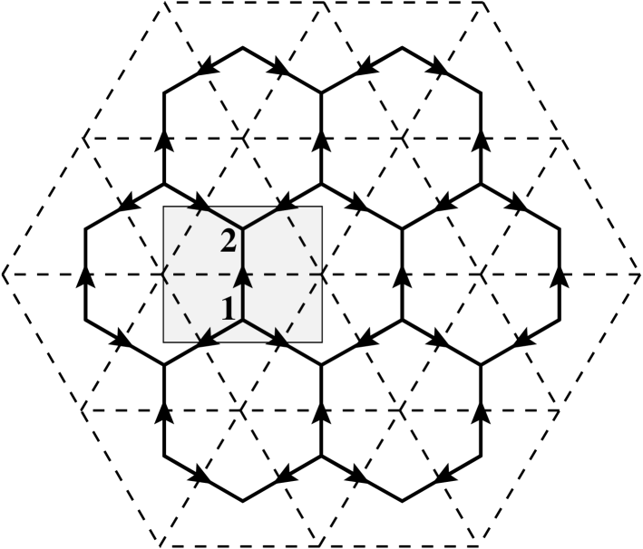
Figure 3: Triangular lattice (dashed lines) and its dual honeycomb lattice (solid lines). The shaded region indicates the two-site unit cell taken for the honeycomb, with the bottom site labeled “1” and the top site “2”.

The boson number and phase are related to the dual fields as follows:

$$n_{\bf r} = \frac{1}{2\pi}(\Delta\times a)_{\bf r}\equiv\frac{1}{2\pi}\sum_{\langle{\bf xx^{\prime}}\rangle\in p_{\bf r}}\!\!\!\!\!\!\!\!\!\!\!\!\!\!\circlearrowleft\>\>a_{\bf xx^{\prime}}$$ (27)

$$e^{i\phi_{\bf r}} = \prod_{\bf r}^{\infty}\!\!\!\!\!\!\!\!\!\!\longrightarrow e^{2\pi i\tilde{e}_{\bf xx^{\prime}}}.$$ (28)

On the right side of Eq. (27), the sum is over the counterclockwise-oriented links of the dual plaquette $p_{\bf r}$ enclosing site ${\bf r}$ of the triangular lattice. The product in Eq. (28) is carried out over an arbitrary string running along the triangular lattice from site ${\bf r}$ to spatial infinity. A factor of $e^{2\pi i\tilde{e}_{\bf xx^{\prime}}}$ appears in the product for every link on the dual lattice bisected by the string, with ${\bf x}$ on the “right” side of the string and ${\bf x^{\prime}}$ on the “left”.

To ensure the uniqueness of the phases $\phi_{\bf r}$ obtained from Eq. (28), the dual Hilbert space is constrained so that the operator

$$N_{\bf x}\equiv(\Delta\cdot\tilde{e})_{\bf x}=\sum_{\bf x^{\prime}}\tilde{e}_{\bf xx^{\prime}}$$ (29)

has integer eigenvalues for all ${\bf x}$. On the right-side of Eq. (29), the sum is over the three nearest-neighbor sites of ${\bf x}$. The meaning of ${N}_{\bf x}$ can be understood by using Eq. (28) to show that

$$N_{\bf x}=\frac{1}{2\pi}\sum_{\langle{\bf rr^{\prime}}\rangle\in p_{\bf x}}\!\!\!\!\!\!\!\!\!\!\!\!\!\!\circlearrowleft\>\>(\phi_{\bf r^{\prime}}-\phi_{\bf r})_{[-\pi,\pi)},$$ (30)

where the sum is over the counterclockwise-oriented links of the triangular plaquette $p_{\bf x}$ enclosing site ${\bf x}$ and the phase difference between adjacent sites is taken to lie in the interval $[-\pi,\pi)$. The eigenvalues of this operator therefore encode vorticity, i.e., the winding number of the phase around the triangular plaquette enclosing ${\bf x}$.

To complete the duality transformation, define a static electric field $e^{0}_{\bf xx^{\prime}}$ related to the vector potential ${\cal A}^{0}_{\bf rr^{\prime}}$ of Eq. (11) by

$$e^{0}_{\bf xx^{\prime}}=-\frac{1}{2\pi}{\cal A}^{0}_{\bf rr^{\prime}},$$ (31)

where $e^{0}_{\bf xx^{\prime}}$ and ${\cal A}^{0}_{\bf rr^{\prime}}$ live on intersecting links of the honeycomb and triangular lattices. Since ${\cal A}^{0}_{\bf rr^{\prime}}$ generates $\pi$ flux per plaquette of the triangular lattice, we require $(\Delta\cdot e^{0})_{\bf x}$ to be half-integer valued. A convenient gauge choice we will now employ is ${\cal A}^{0}_{\bf rr^{\prime}}=\pm\pi/3$ on each nearest-neighbor link, directed clockwise around “up” triangles and counterclockwise around “down” triangles. In this gauge, $e^{0}_{\bf xx^{\prime}}=1/6$ along the arrows shown in Fig. 3 so that $(\Delta\cdot e^{0})_{\bf x}=+1/2$ on sublattice 1 while $(\Delta\cdot e^{0})_{\bf x}=-1/2$ on sublattice 2.

Upon defining $e_{\bf xx^{\prime}}\equiv\tilde{e}_{\bf xx^{\prime}}-e_{\bf xx^{\prime}}^{0}$ we thereby arrive at a simple form for the dual Hamiltonian,

$${\mathcal{H}}=-J\sum_{\langle{\bf xx^{\prime}}\rangle}\cos(2\pi e_{\bf xx^{\prime}})+U^{\prime}\sum_{\bf r}(\Delta\times a)_{\bf r}^{2},$$ (32)

with $U^{\prime}=U/(2\pi)^{2}$. This Hamiltonian is supplemented by the constraint that,

$$(\Delta\cdot e)_{\bf x}=N_{\bf x}-1/2,$$ (33)

where we have found it convenient to shift the integer field $N_{\bf x}\rightarrow N_{\bf x}-1$ for all ${\bf x}$ on sublattice 2.

As it stands, this Hamiltonian is difficult to work with due to the integer constraint on the field $a_{\bf xx^{\prime}}/(2\pi)$. It is therefore highly desirable to “soften” this constraint, allowing $a_{\bf xx^{\prime}}$ to roam over all real numbers. To be consistent $e_{\bf xx^{\prime}}$ must also be taken on the real numbers, and it is then legitimate to expand the cosine term in Eq. (32) to obtain,

$$\tilde{\mathcal{H}} = \sum_{\langle{\bf xx^{\prime}}\rangle}[J^{\prime}e_{\bf xx^{\prime}}^{2}-2t_{v}\cos(\theta_{\bf x}-\theta_{\bf x^{\prime}}-a_{\bf xx^{\prime}})]$$ (34)

$$+ U^{\prime}\sum_{\bf r}(\Delta\times a)_{\bf r}^{2},$$

with $J^{\prime}\approx 2\pi^{2}J$. Here we have added a cosine term acting on the field $a_{\bf xx^{\prime}}$ to implement the integer constraint softly, and explicitly expressed the longitudinal piece of $a_{\bf xx^{\prime}}$ as a lattice derivative of a “phase” field $\theta_{\bf x}\in[-\pi,\pi)$ living on the dual lattice sites. The dual Hilbert space satisfies the constraint Eq. (33) with the vortex number operator $N_{\bf x}\in{\mathbb{Z}}$ conjugate to $\theta_{\bf x}$. The operator $e^{i\theta_{\bf x}}$ creates a vortex at site ${\bf x}$ and satisfies the commutation relations $[N_{\bf x},e^{i\theta_{\bf x^{\prime}}}]=\delta_{\bf xx^{\prime}}e^{i\theta_{\bf x}}$. The $t_{v}$ term above thus allows nearest-neighbor vortex hopping in addition to energetically favoring integer values for the density $n_{\bf r}$.

Generically, we should also allow short-range vortex interaction of the form

$$\sum_{\bf xx^{\prime}}(N_{\bf x}-1/2)V^{\rm sr}_{\bf xx^{\prime}}(N_{\bf x^{\prime}}-1/2),$$ (35)

in addition to the retarded long-range interaction mediated by the gauge fields. For a static configuration of vortices or in the instantaneous limit when the “speed of light” $(U^{\prime}/J^{\prime})^{1/2}$ is infinite, the latter interaction becomes a 2D lattice Coulomb potential varying as $V^{\rm Coul}_{\bf xx^{\prime}}\sim-J^{\prime}\ln|{\bf x}-{\bf x^{\prime}}|$.

III.2 Phases in the Dual Vortex Variables

Physically, the dual Hamiltonian describes vortices hopping on the sites of the dual honeycomb lattice, interacting via a 2D “electromagnetic” interaction. Most importantly, the vortices are at half-filling, which can be directly traced to the frustration on the original triangular lattice plaquettes. This highlights the distinction between the triangular lattice XY antiferromagnet and its unfrustrated counterparts, which have a dual vortex theory with an integer mean vortex number.

To illuminate the challenge in treating the strongly interacting vortex system when at half-filling, it is instructive to consider how the various phases of the original model are described in terms of the dual variables. The magnetically-ordered states correspond to “insulating” phases of the dual vortices. For example, the ordered phase with $120^{\circ}$ coplanar order of the XY spins corresponds to a “vortex density wave” state in which the vortices sit preferentially on one of the two sublattices of the dual honeycomb lattice. On the other hand, the ordered states with collinear order correspond to “vortex valence bond” phases; one signature of these phases is the bond energy density order, which can be measured both in terms of the vortices and in terms of the original spins. Specifically, the bond energy wave operator for the vortices takes a similar form as in Eq. (20), except with the vortex bond energy operator inserted,

$$B_{{\bf rr}^{\prime}}\sim e^{i{\bf Q}\cdot({\bf r}+{\bf r^{\prime}})}\cos(\theta_{\bf x}-\theta_{\bf x^{\prime}}-a_{\bf xx^{\prime}})~{}.$$ (36)

Here, the nearest-neighbor pairs ${\bf r}$, ${\bf r^{\prime}}$ and ${\bf x}$, ${\bf x^{\prime}}$ are bridged by intersecting links of the triangular and honeycomb lattices.

In all of these magnetically-ordered phases, since the dual vortices are “insulating” and immobile, the “photon” in the dual fields $a_{\bf xx^{\prime}}$ and $e_{\bf xx^{\prime}}$ can freely propagate. This “photon” mode corresponds to the Goldstone spin-wave mode of the original XY spins. On the other hand, the paramagnetic phase for the XY spins corresponds to a phase within which the dual vortices have condensed, $\langle e^{i\theta_{\bf x}}\rangle\neq 0$. In this dual vortex “superfluid” the dual gauge flux is expelled, and the dual gauge field $a_{\bf xx^{\prime}}$ picks up a Higgs mass; thus, the spectrum is gapped in this phase as expected in the spin paramagnet.

The quantum phase transitions separating the paramagnet from the coplanar and collinear ordered spin states correspond to “superfluid-insulator” transitions for the dual vortices. But all of these vortex “insulators” involve a spontaneous breaking of lattice translational symmetries, due to the fact that the vortices are at half-filling. Due to these complications it is not at all clear how one can possibly access the critical properties of these transitions from this dual vortex formulation. In the next section we demonstrate how this can be achieved, by fermionizing the vortices. Before undertaking this rather tricky business, we first summarize how the vortex fields transform under all of the lattice and internal symmetries.

III.3 Symmetry Transformations for Vortices

The transformation properties of the dual vortex and gauge fields can be deduced upon inspection of their defining equations, Eqs. (27) and (28), together with the transformation properties of the rotor fields $\phi_{\bf r}$ and $n_{\bf r}$. For example, lattice translations $T_{\bf\delta r}$ and $\pi/3$ rotations $R_{\pi/3}$ transform the dual coordinates (e.g., ${\bf x}\rightarrow{\bf x}+{\bf\delta r}$ under $T_{\bf\delta r}$), but do not transform the dual gauge fields $a,e$ or vortex fields $\theta,N$ as shown in Table 2. Here and in what follows, our coordinate origin is always at a triangular lattice site. Under charge conjugation ${\mathcal{C}}$, however, the fields $a,e,\theta$ change sign while $N\rightarrow 1-N$. Similarly, time reversal ${\mathcal{T}}$ changes the sign of the dual fields $a,\theta$ but leaves $e,N$ unchanged. Since ${\cal T}$ is accompanied by complex conjugation the vortex creation operator $e^{i\theta}$ remains invariant under time reversal.

For lattice reflections it is convenient for later developments to henceforth consider a modified (antiunitary) transformation, $\tilde{\cal R}_{x}$, which is defined as ${\cal R}_{x}$ combined with ${\cal C}$ and ${\cal T}$:

$$\tilde{\cal R}_{x}\equiv{\cal R}_{x}{\cal C}{\cal T}.$$ (37)

The dual fields transform under $\tilde{\mathcal{R}}_{x}$ in the same way they transform under time reversal, with the dual coordinates additionally $x$-reflected. The complete set of symmetry transformations for the dual fields is summarized in Table 2.

Finally, we remark that the global $U(1)$ or XY spin symmetry corresponding to $e^{i\phi}\rightarrow e^{i(\phi+\alpha)}$ is not directly manifest in the dual vortex formulation, as can be seen by examining Eq. (28). This global $U(1)$ symmetry reflects the underlying conservation of the boson number $n_{\bf r}$ (or the $S^{z}$-component of spin) and is replaced in the dual formulation by the conservation of the dual flux $(\Delta\times a)_{\bf r}$. Note also that the dual theory has a $U(1)$ gauge redundancy (not a physical symmetry) given by $a_{\bf xx^{\prime}}\to a_{\bf xx^{\prime}}+\Lambda_{\bf x}-\Lambda_{\bf x^{\prime}}$ and $\theta_{\bf x}\to\theta_{\bf x}+\Lambda_{\bf x}$, where $\Lambda_{\bf x}\in{\mathbb{R}}$.

Table 2: Transformation properties of the dual fields under the microscopic symmetries. For brevity, the lattice coordinates, which also transform appropriately under the lattice symmetries, have been suppressed on all fields. Here we use a modified reflection $\tilde{\mathcal{R}}_{x}$, which is a combination of ${\mathcal{R}}_{x}$, ${\mathcal{C}}$, and ${\mathcal{T}}$. Both ${\cal T}$ and $\tilde{\cal R}_{x}$ are accompanied with a complex conjugation, so that e.g. $e^{i\theta}$ is invariant.

$T_{{\bf\delta r}}$, $R_{\pi/3}$	${\mathcal{C}}$	$\tilde{\mathcal{R}}_{x}$, ${\mathcal{T}}$
$a\rightarrow a$	$a\rightarrow-a$	$a\rightarrow-a$
$e\rightarrow e$	$e\rightarrow-e$	$e\rightarrow e$
$\theta\rightarrow\theta$	$\theta\rightarrow-\theta$	$\theta\rightarrow-\theta$
$N\rightarrow N$	$N\rightarrow 1-N$	$N\rightarrow N$

IV Fermionization of vortices

IV.1 Chern-Simons Flux Attachment

As described in Sec. III.2, an analysis of the phase transitions in the dual bosonic vortex theory is highly nontrivial because the vortices are at half-filling, and we do not know how to formulate a continuum theory of such bosonic degrees of freedom. We will sidestep difficulties associated with the finite vortex density by fermionizing the vortices, which as we will demonstrate enables one to make significant progress in this direction. Specifically, we first treat the vortices as hard-core bosons, with the identification

$$b_{\bf x}^{\dagger}\sim e^{i\theta_{\bf x}},\quad N_{\bf x}=b_{\bf x}^{\dagger}b_{\bf x}=0,1~{}.$$ (38)

This is a reasonable approximation due to the repulsive vortex interactions, and the hard-core condition does not affect generic behavior. We then perform a two-dimensional Jordan-Wigner transformationFradkin (1989),

$$b_{\bf x}^{\dagger} = d_{\bf x}^{\dagger}\exp[i\sum_{{\bf x}^{\prime}\neq{\bf x}}\arg({\bf x},{\bf x}^{\prime})N_{{\bf x}^{\prime}}],$$ (39)

$$N_{\bf x} = b_{\bf x}^{\dagger}b_{\bf x}=d_{\bf x}^{\dagger}d_{\bf x}.$$ (40)

Here, $\arg({\bf x},{\bf x}^{\prime})$ is an angle formed by the vector ${\bf x}-{\bf x}^{\prime}$ with some fixed axis. It is simple to check that $d_{\bf x}$ are fermionic operators satisfying the anticommutation relations $\{d_{\bf x},d_{{\bf x}^{\prime}}^{\dagger}\}=\delta_{{\bf x}{\bf x}^{\prime}}$. The vortex hopping part of the Hamiltonian becomes

$$-t_{v}\sum_{\langle{\bf x}_{1}{\bf x}_{2}\rangle}[d_{{\bf x}_{1}}^{\dagger}d_{{\bf x}_{2}}e^{-iA_{{\bf x}_{1}{\bf x}_{2}}}e^{-ia_{{\bf x}_{1}{\bf x}_{2}}}+{\rm h.c.}]~{}.$$ (41)

The Chern-Simons field

$$A_{{\bf x}_{1}{\bf x}_{2}}\equiv\sum_{{\bf x}^{\prime}\neq{\bf x}_{1},{\bf x}_{2}}[\arg({\bf x}_{2},{\bf x}^{\prime})-\arg({\bf x}_{1},{\bf x}^{\prime})]N_{{\bf x}^{\prime}}$$ (42)

lives on the links of the honeycomb lattice and is completely determined by the positions of the particles. In this transformation, we have essentially expressed hard-core bosons on the lattice as fermions each carrying a fictitious $2\pi$ flux. We used the Hamiltonian language in order to facilitate our discussion of the discrete symmetries below.

The Chern-Simons field satisfies

$$(\Delta\times A)_{\bf r}=\frac{2\pi}{3}\sum_{{\bf x}\in p_{\bf r}}(N_{\bf x}-1/2),$$ (43)

i.e., the fictitious $2\pi$ flux attached to a fermion can be viewed as equally-shared among its three adjacent plaquettes. In the above equation, we subtracted $1/2$ from each $N_{\bf x}$ to remove an unimportant $2\pi$ flux from each hexagon. This constitutes a convenient choice such that the Chern-Simons flux piercing the dual lattice vanishes on average since the vortices are half-filled. There are further restrictions on the Chern-Simons field which we write schematically as $\Delta\cdot A=0$ appropriate in the continuum limit.

The complete Hamiltonian describes half-filled fermions with nearest-neighbor hopping on the honeycomb lattice, coupled to the $U(1)$ gauge field $a_{{\bf x}{\bf x}^{\prime}}$ and the Chern-Simons field $A_{{\bf x}{\bf x}^{\prime}}$. We can crudely say that the gauge field $a_{{\bf x}{\bf x}^{\prime}}$ gives rise to repulsive logarithmic interactions between the fermions.

Under the microscopic symmetries, the fields in this fermionized representation transform as shown in Table 3. The symmetry properties of the fermion operators under translation, rotation, and modified reflection are readily obtained by inspecting Eq. (39) (throughout, we ignore a possible global $U(1)$ phase). In each case, the transformation of the Chern-Simons field is obtained from Eq. (42).

Table 3: Symmetry transformation properties of the fields in the fermionized representation. The transformation properties of $a,e$ are the same as in Table 2. In the ${\mathcal{C}}$ column, $j=1,2$ refers to the sublattice index on the honeycomb lattice (site index in the unit cell pictured in Fig. 3). The additional column ${\mathcal{T}}_{\rm ferm}$ corresponds to the naïve time reversal for the lattice fermions and is not a symmetry of the vortex Hamiltonian.

	$T_{\delta{\bf r}}$, $R_{\pi/3}$	$\tilde{\mathcal{R}}_{x}$	${\mathcal{C}}$	${\mathcal{T}}$	${\mathcal{T}_{\rm ferm}}$
$a\to$	$a$	$-a$	$-a$	$-a$	$-a$
$e\to$	$e$	$e$	$-e$	$e$	$e$
$d_{\bf x}\to$	$d$	$d$	$(-1)^{j}d^{\dagger}$	$d_{\bf x}e^{-2i\sum_{{\bf x}^{\prime}\neq{\bf x}}\arg({\bf x},{\bf x}^{\prime})N_{{\bf x}^{\prime}}}$	$d$
$A\to$	$A$	$-A$	$-A$	$A$

Charge conjugation and time reversal require some explanation. From Eq. (39), we have for particle-hole

$${\cal C}:d_{\bf x}\to d_{\bf x}^{\dagger}\exp[i\sum_{{\bf x}^{\prime}\neq{\bf x}}\arg({\bf x},{\bf x}^{\prime})]=d_{\bf x}^{\dagger}\exp[i\gamma_{\bf x}]~{}.$$ (44)

The phase $\gamma_{\bf x}$ is constant in time but depends on the lattice site. For two nearest-neighbor sites on the honeycomb lattice we have

$$\gamma_{{\bf x}_{1}}-\gamma_{{\bf x}_{2}} = \arg({\bf x}_{1},{\bf x}_{2})-\arg({\bf x}_{2},{\bf x}_{1})$$

$$+\sum_{{\bf x}^{\prime}\neq{\bf x}_{1},{\bf x}_{2}}[\arg({\bf x}_{1},{\bf x}^{\prime})-\arg({\bf x}_{2},{\bf x}^{\prime})]$$

$$= \pi-2A_{{\bf x}_{1}{\bf x}_{2}}[N_{{\bf x}^{\prime}}\equiv 1/2]~{}.$$

With our convention in Eq. (43) where the Chern-Simons field fluctuates around zero, we conclude that $e^{i\gamma_{\bf x}}$ changes sign going between nearest neighbors. The resulting $e^{i\gamma_{\bf x}}$ is written as $(-1)^{j}$ in Table 3, where $j=1,2$ refers to the sublattice index of site ${\bf x}$.

Finally, time reversal acts as

$${\cal T}:d_{\bf x}\to d_{\bf x}\exp[-2i\sum_{{\bf x}^{\prime}\neq{\bf x}}\arg({\bf x},{\bf x}^{\prime})N_{{\bf x}^{\prime}}].$$ (45)

This is a formally exact implementation of the symmetry, but the phases multiplying the fermion operators now depend on the positions of all the vortices. This nonlocal transformation represents a serious difficulty once we derive a low-energy continuum theory in the next subsection. In particular, it will not be possible to correctly represent the time-reversal transformation ${\cal T}$ using only the continuum fields. Since our treatment below will involve crucial assumptions regarding this issue, it is useful to also give a formulation of time-reversal symmetry in first-quantized language. Focusing on the particle degrees of freedom, the Jordan-Wigner transformation expresses the wavefunction for the bosonic vortices as

$$\Psi_{\rm boson}({\bf x}_{1},{\bf x}_{2},\dots)=\prod_{i<j}e^{-i\arg({\bf x}_{i},{\bf x}_{j})}\;\;\Psi_{\rm ferm}({\bf x}_{1},{\bf x}_{2},\dots)~{}.$$ (46)

When the Chern-Simons phase factor is not affected by a symmetry transformation, the properties of the bosonic and fermionic wavefunctions coincide under the transformation. However, time reversal sends $i\to-i$, hence the requirement that the bosonic wavefunction is real implies that

$$\Psi^{*}_{\rm ferm}({\bf x}_{1},{\bf x}_{2},\dots)=\prod_{i<j}e^{-2i\arg({\bf x}_{i},{\bf x}_{j})}\;\;\Psi_{\rm ferm}({\bf x}_{1},{\bf x}_{2},\dots)~{}.$$ (47)

Thus, the time-reversal invariance of the bosonic wave function is a highly nontrivial condition for the fermionic wavefunction.

For this reason, it is convenient to define a modified time-reversal transformation, which corresponds to naïve time reversal for the lattice fermions:

$${\cal T}_{\rm ferm}:\quad d_{\bf x}\to d_{\bf x};\quad a\to-a;\quad e\to e;\quad i\to-i.$$ (48)

In first-quantized language ${\cal T}_{\rm ferm}$ corresponds to complex conjugation of the wavefunction for the fermionized vortices, $\Psi_{\rm ferm}\to\Psi^{*}_{\rm ferm}$. It is important to emphasize that this transformation is not a symmetry of the fermionic Hamiltonian, since under ${\cal T}_{\rm ferm}$ the field $a$ changes sign while the Chern-Simons field $A$ from Eq. (42) remains unchanged.

However, as we shall argue further below, since the vortices interact logarithmically, their density fluctuations are greatly suppressed, and it is plausible that the phase factors in Eqs. (45) and (47) might be essentially the same for all vortex configurations that carry substantial weight. For an extreme example, if the vortices form a perfect charge-ordered state, then the Chern-Simons phase factor is constant. We conjecture below that this is also the case at the critical points separating the spin-ordered states from the spin paramagnet. In any event, in situations where the Chern-Simons phase factors are roughly constant for all important configurations, the physical and modified time-reversal transformations become essentially identical. It is then legitimate to require that the theory be invariant under ${\cal T}_{\rm ferm}$. This will be useful when we describe a conjectured low-energy continuum fermionic theory for criticality in the vortex system, since ${\cal T}_{\rm ferm}$ acts in a simple, local way on the continuum fermion fields.

IV.2 Naïve Continuum Theory

To arrive at a low-energy continuum theory, we first consider a “flux-smeared” mean-field state with $A_{{\bf x}{\bf x}^{\prime}}=0$. We will also ignore fluctuations in $a_{{\bf x}{\bf x}^{\prime}}$ for the moment, taking $a_{{\bf x}{\bf x}^{\prime}}=0$. We are then left with half-filled fermions hopping on the honeycomb lattice with no fluxes.

Diagonalizing the hopping Hamiltonian in momentum space using the two-site unit cell shown in Fig. 3, one finds that there are two Dirac points at momenta $\pm{\bf Q}$, where ${\bf Q}=(4\pi/3,0)$. (Note that these are the same wavevectors found for the low-energy spin-1 excitations in the continuum analysis of the original spin model in Sec. II.2.) Focusing only on low-energy excitations in the vicinity of these momenta, the fermion operators can be expanded around the Dirac points. Denoting the lattice fermion field on the two sublattices as $d_{{\bf x}\alpha}$ with $\alpha=1,2$ the sublattice label, we write

$$d_{{\bf x}\alpha}\approx\psi_{R\alpha}e^{i{\bf Q}\cdot{\bf x}}+i\sigma_{\alpha\beta}^{y}\psi_{L\beta}e^{-i{\bf Q}\cdot{\bf x}},$$ (49)

where ${\bf x}$ continues to label the real-space position of the honeycomb lattice site and $\sigma^{y}$ is a Pauli matrix. The fields $\psi_{R/L}$ are two-component spinors that vary slowly on the lattice scale. Using this expansion we obtain for the free-fermion part of the continuum Hamiltonian

$$H_{f}^{(0)}=\int d{\bf x}\;\psi_{a}^{\dagger}\,v\,(p_{x}\sigma^{x}+p_{y}\sigma^{y})\psi_{a}~{},$$ (50)

where ${\bf p}=-i\bm{\nabla}$ is the momentum operator, an implicit summation over the flavor index $a\in[R,L]$ is understood, and we have suppressed the summation over the spinor indices $\alpha,\beta$. From now on, we absorb the nodal velocity $v$ in the scaling of the coordinates.

It is convenient to work in the Euclidean path integral description. The free-fermion Lagrangian density is written in the form

$${\mathcal{L}}_{f}^{(0)} = \overline{\psi}_{a}\gamma^{\mu}\partial_{\mu}\psi_{a},$$ (51)

$$\overline{\psi}_{R/L} \equiv \psi_{R/L}^{\dagger}\gamma^{0},$$ (52)

with implicit sums over the flavor index $a\in[R,L]$ and space-time index $\mu\in[0,1,2]$, defined so that $\partial_{0,1,2}\equiv\partial_{\tau,x,y}$. The $2\times 2$ Dirac matrices $\gamma^{\mu}$ are given by $\gamma^{0}=\sigma^{z}$, $\gamma^{1}=\sigma^{y}$, $\gamma^{2}=-\sigma^{x}$ and satisfy the usual algebra $\{\gamma^{\mu},\gamma^{\nu}\}=2\delta^{\mu\nu}$. These matrices act within each two-component field so that $(\gamma^{\mu}\psi_{a})_{\alpha}\equiv\gamma^{\mu}_{\alpha\beta}\psi_{a\beta}$. We will also find it useful to define Pauli matrices $\tau^{x,y,z}$ that act on the $R/L$ flavor indices, i.e., $(\tau^{k}\psi)_{a\alpha}\equiv\tau^{k}_{ab}\psi_{b\alpha}$.

Including the gauge-field fluctuations and the short-range fermion interactions, we arrive at a Lagrangian of the form

$${\mathcal{L}} = \overline{\psi}_{a}\gamma^{\mu}(\partial_{\mu}-ia_{\mu}-iA_{\mu})\psi_{a}$$ (53)

$$+ \frac{1}{2e^{2}}(\epsilon_{\mu\nu\lambda}\partial_{\nu}a_{\lambda})^{2}+\frac{i}{4\pi}\epsilon_{\mu\nu\lambda}A_{\mu}\partial_{\nu}A_{\lambda}+{\mathcal{L}}_{\rm 4f}.$$

Here $\epsilon_{\mu\nu\lambda}$ is the anti-symmetric tensor, and for simplicity we wrote a space-time isotropic form for the Maxwell action of the gauge field $a_{\mu}$. We also used the standard $(2+1)$-dimensional form for the Chern-Simons action that ensures the attachment of $2\pi$ flux to the fermions, restoring the bosonic exchange statistics of the vortices. In the absence of the four-fermion terms ${\mathcal{L}}_{4f}$, there is a global $SU(2)$ flavor symmetry, whose action on the fermion fields is generated by the $\tau^{k}$ Pauli matrices.

The four-fermion interaction terms can be written as

$${\mathcal{L}}_{4f}=\lambda_{0}J_{0}^{2}+\lambda_{z}J_{z}^{2}+\lambda_{\perp}(J_{x}^{2}+J_{y}^{2})+\lambda^{\prime}_{0}(\overline{\psi}_{a}\gamma^{0}\psi_{a})^{2},$$ (54)

where we have defined a flavor $SU(2)$ vector of fermion bilinears,

$$\bm{J}\equiv\overline{\psi}_{a}{\bm{\tau}}_{ab}\psi_{b}=\psi^{\dagger}_{a}\sigma^{z}{\bm{\tau}}_{ab}\psi_{b}~{},$$ (55)

and a “mass term,”

$$J_{0}\equiv\overline{\psi}_{a}\psi_{a}=\psi^{\dagger}_{a}\sigma^{z}\psi_{a}~{}.$$ (56)

The four-fermion terms arise from vortex density-density interactions and other short-range interaction processes. For example, the $\lambda_{0}^{\prime}$ term roughly represents an overall vortex repulsion, while the $\lambda_{z}$ term represents the difference in repulsion between vortices on the same sublattice and opposite sublattices of the honeycomb. ${\mathcal{L}}_{4f}$ contains all independent four-fermion terms that can arise from the microscopic short-range fermion interactions (including possible short-range pieces mediated by the gauge fields).

The above constitutes the naïve continuum limit obtained by inserting the slow-field expansion Eq. (49) into the microscopic Hamiltonian and assuming small fluctuations in the gauge field $a$ and the Chern-Simons field $A$. We now discuss the symmetries of the continuum formulation. Table 4 shows the transformation properties of the continuum fermion fields deduced from the lattice fermion transformations in Table 3. Also shown are the symmetry transformation properties of the fermion bilinears $\bm{J}$ and $J_{0}$. Missing from the table is the original time-reversal invariance, which we do not know how to realize in the continuum. In its place we have included the modified time reversal ${\cal T}_{\rm ferm}$, defined in Eq. (48), which corresponds to the naïve time-reversal transformation for fermions hopping on the honeycomb lattice. Remarkably, the transformation properties of the flavor $SU(2)$ vector $\bm{J}$ of fermionic bilinears are identical to the transformation properties of the bosonic flavor $SU(2)$ vector defined in Sec. II.2, $\bm{K}=\Phi^{*}_{a}\bm{\tau}_{ab}\Phi_{b}$. Surprisingly, the fermionic bilinear $\bm{J}$ transforms under the modified time-reversal transformation ${\cal T}_{\rm ferm}$ in precisely the way that the bosonic bilinear $\bm{K}$ transforms under the physical time reversal ${\cal T}$.

Table 4: Transformation properties of the continuum fermion fields $\psi_{R/L}$ and the fermion bilinears $\bm{J}$, $J_{0}$ under the microscopic symmetries. Here $J_{\pm}=J_{x}\pm iJ_{y}$. The spatial coordinates, which should transform appropriately under the lattice symmetries, have been suppressed for conciseness. The last column does not correspond to the physical time-reversal symmetry, which we cannot realize in a local manner in the continuum theory. Rather, it corresponds to the naïve time reversal in Eq. (48) for fermions hopping on the honeycomb lattice.

	$T_{\bf\delta r}$	$R_{\pi/3}$	$\tilde{\cal R}_{x}$	${\mathcal{C}}$	${\cal T}_{\rm ferm}$
$\psi\to$	$e^{i{\bf Q\cdot\delta r}\tau^{z}}\psi$	$i\tau^{x}e^{-i\pi\sigma^{z}/6}\psi$	$\psi$	$\tau^{x}\sigma^{x}[\psi^{\dagger}]^{t}$	$i\tau^{y}\,i\sigma^{y}\psi$
$J_{z}\to$	$J_{z}$	$-J_{z}$	$J_{z}$	$-J_{z}$	$J_{z}$
$J_{\pm}\to$	$e^{\mp 2i{\bf Q\cdot\delta r}}J_{\pm}$	$J_{\mp}$	$J_{\pm}$	$J_{\pm}$	$J_{\mp}$
$J_{0}\to$	$J_{0}$	$J_{0}$	$J_{0}$	$J_{0}$	$-J_{0}$

One can verify that the first four symmetries in Table 4 (translation, rotation, modified reflection, and particle-hole) preclude all quartic fermion terms from the Lagrangian except the four terms exhibited in Eq. (54). Moreover, these symmetries prohibit all fermionic bilinears in the Lagrangian except a mass term of the form $MJ_{0}=M\overline{\psi}\psi$. This merits some discussion. In situations where it is legitimate to replace the time-reversal transformation by the modified symmetry ${\cal T}_{\rm ferm}$, we can use this modified symmetry to preclude such a mass term. However, generally this might not be possible. Indeed, as we shall see in the next subsection, a large mass term of this form when added to the Lagrangian places the system in the spin paramagnetic phase, provided the mass $M$ has a specific sign relative to the Chern-Simons term. Since we know that the spin paramagnet does not break time-reversal symmetry ${\cal T}$, it is clear that at least in this phase it is not legitimate to replace ${\cal T}$ with ${\cal T}_{\rm ferm}$. The reasons for this will become clear in the next subsection where we describe how the spin paramagnet and the spin ordered phases can be correctly described using the fermionized-vortex formulation. The discussion of whether or not it is legitimate to replace ${\cal T}$ with ${\cal T}_{\rm ferm}$ at the critical points separating these phases will be deferred until Sec. IV.4.

IV.3 Phases in the Fermionic Representation

We now discuss how to recover the phases of the original spin model using the fermionic vortex fields. This extends our earlier discussion using the bosonic vortices in Sec. III.2. The paramagnetic phase of the original spin model is the bosonic vortex superfluid (Higgs) phase. In terms of the fermionic vortex fields, the paramagnet is obtained as an integer quantum Hall state, which in the continuum description corresponds to the presence of a mass term $M\overline{\psi}\psi$. Both fermion fields $\psi_{R}$ and $\psi_{L}$ then have the same mass $M$ with the same sign. Let us see that we indeed recover the correct description of the original spin paramagnet. Integrating out the massive fermions induces a Chern-Simons term for the sum field $(a+A)_{\mu}$, so the Lagrangian for the fields $a_{\mu}$ and $A_{\mu}$ becomes

$${\cal L}_{a,A} = \frac{1}{2e^{2}}(\epsilon_{\mu\nu\lambda}\partial_{\nu}a_{\lambda})^{2}+\frac{i}{4\pi}\epsilon_{\mu\nu\lambda}A_{\mu}\partial_{\nu}A_{\lambda}$$ (58)

$$+\frac{i\text{sign}(M)}{4\pi}\epsilon_{\mu\nu\lambda}(a+A)_{\mu}\partial_{\nu}(a+A)_{\lambda}~{}.$$

We now stipulate that the sign of the mass $M$ is taken to cancel the original Chern-Simons term for the field $A$. One can then verify that the spectrum corresponding to the above Lagrangian is gapped. For example, upon integrating out $A$ the gauge field $a$ obtains a mass. This is as expected, since there are no gapless excitations in this phase. Gapped quasiparticles of the paramagnetic phase of the spin model are described as follows. Consider acting with the fermion field $\psi_{R/L}^{\dagger}$ on the ground state. This is essentially the same as inserting a vortex in the vortex field $\theta$. The added fermion couples to $a+A$, and by examining ${\cal L}_{a,A}$ we find that it binds $\nabla\!\times\!a=-2\pi$ flux to the fermion. Thus, the fermion is turned into a localized bosonic excitation, which is the familiar screened vortex in the vortex field $\theta$ (the sign of the flux is of course consistent with our minimal coupling convention ${\bm{\nabla}}\theta+{\bm{a}}$). In terms of the original spin model, this bosonic excitation carries spin 1 and is precisely the magnon of the paramagnet.

It is worth remarking about the role of time-reversal symmetry and the modified time-reversal transformation ${\cal T}_{\rm ferm}$ of Eq. (48) in the spin paramagnetic phase. Since the spin paramagnet corresponds to an integer quantum Hall state for the fermions, it is clear that ${\cal T}_{\rm ferm}$ will not be respected in this phase. This is consistent with Table 4, which shows that the mass term $\overline{\psi}\psi$ is odd under ${\cal T}_{\rm ferm}$. On the other hand, the phase factors in the fermionic integer quantum Hall wavefunction will conspire to cancel the Chern-Simons phase factors in Eq. (47) leading to a wavefunction for the bosonic vortices which is real—consistent with physical time-reversal invariance.

Consider now the magnetically ordered phases of the original spin model. These correspond to vortex insulators and are obtained in the fermionic theory as a result of spontaneously generating a fermion mass of the form

$$\langle\bm{J}\rangle=\langle\overline{\psi}\bm{\tau}\psi\rangle\neq 0~{}.$$ (59)

In the presence of such mass terms we have two massive Dirac fermion fields with opposite-sign masses, and integrating out the fermions produces only a generic Maxwell term for the sum field $(a+A)_{\mu}$. The gapless photon mode of the gauge field $a$ then corresponds to the spin wave of the magnetically-ordered phase. Acting with a fermion creation operator also binds $2\pi$ flux of the Chern-Simons field $A$ and turns the fermion back into the original bosonic vortex. Because of the gapless gauge field $a$ such an isolated vortex costs a logarithmically-large energy as expected in the spin-ordered phase.

Spontaneous mass generation is driven by interaction terms in the Hamiltonian such as the $\lambda_{z}$ and $\lambda_{\perp}$ interactions. The details of the magnetic order are determined by the specific mass term that is generated. For example, the mass term $m_{z}J_{z}$ in the Lagrangian corresponds to the vortex “charge density wave” (CDW) state wherein vortices preferentially occupy one sublattice of the honeycomb lattice as shown in Fig. 4a. Indeed, from Table 4, this mass term is odd under the $\pi/3$ rotation and particle-hole symmetries, and can be identified with a staggered chemical potential for the lattice fermions that selects one of the charge-ordered states over the other. Therefore such spontaneously-generated mass gives rise to the translation symmetry breaking in the vortex system that produces the CDW state. In the original spin model, this corresponds to the coplanar spin state of Fig. 1a.

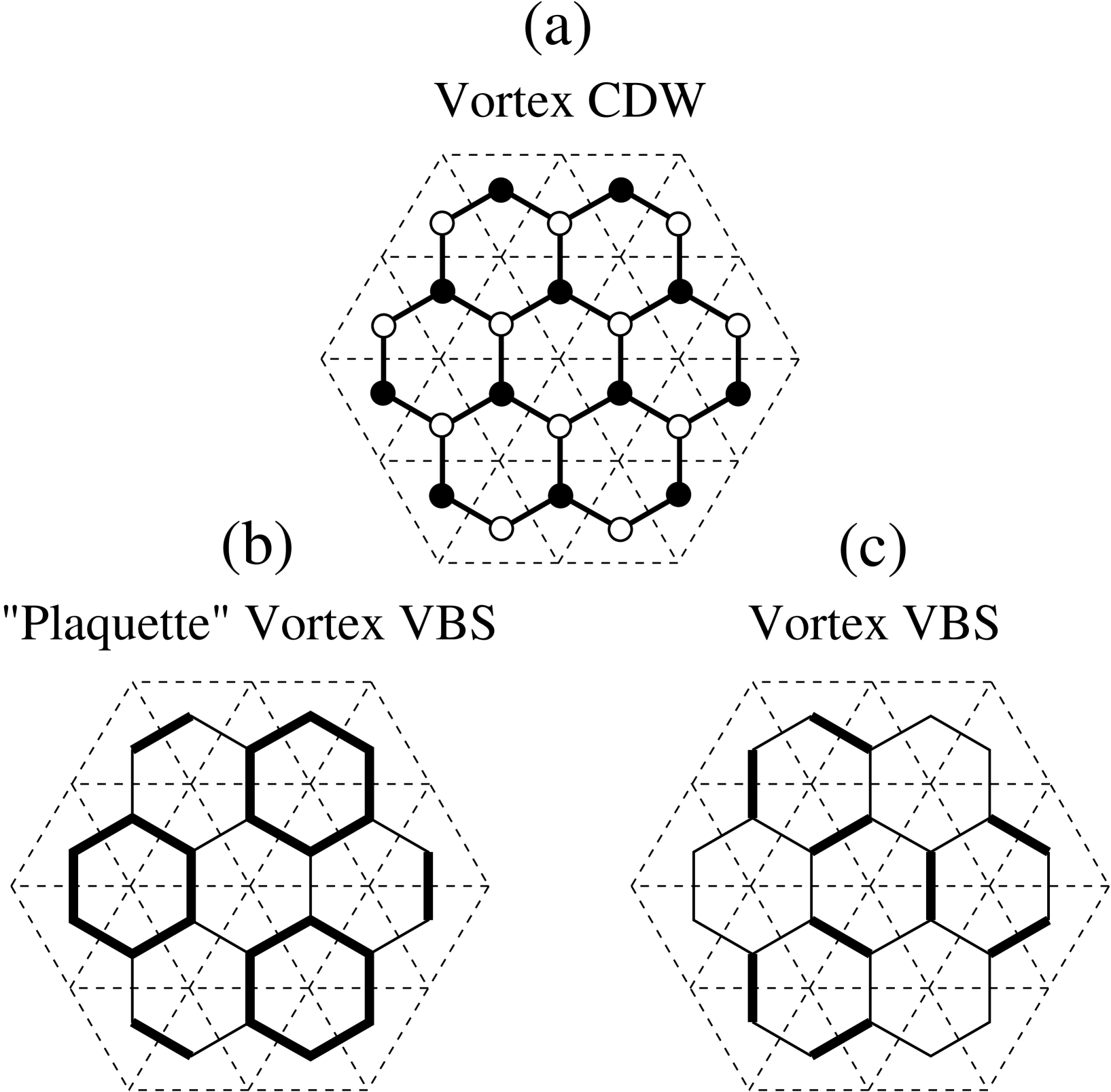
Figure 4: Vortex insulators that correspond to the spin-ordered states of Fig. 1. (a) Staggered vortex “charge density wave” (CDW) state, corresponding to the coplanar $\sqrt{3}\times\sqrt{3}$ state in the original spin variables. Vortices preferentially occupy one of the two sublattices. (b) “Plaquette” vortex valence bond solid (VBS), corresponding to the dice-lattice collinear antiferromagnetic spin order. Vortex density is spread over the bold hexagons. (c) Vortex VBS, corresponding to the hexagonal collinear antiferromagnetic spin order. Vortices preferentially occupy the lattice of bold links.

On the other hand, the mass term $m_{x}J_{x}+m_{y}J_{y}$ corresponds to the vortex valence bond solid (VBS) state. The specific pattern is not resolved with only the four-fermion interactions, but we expect that because of the underlying lattice there are higher-order terms in the action that pin the direction in the $(J_{x},J_{y})$ plane so that $\langle J_{+}\rangle^{3}$ is either $+1$ or $-1$. The corresponding bond orders are deduced by interpreting the spontaneously-generated mass term $|m|(e^{i\alpha}J_{+}+e^{-i\alpha}J_{-})/2$ as inducing a modulated vortex hopping amplitude $t_{{\bf x},{\bf x}^{\prime}}=1+|m|\cos[{\bf Q}\cdot({\bf x}+{\bf x}^{\prime})+\alpha]/2$. For $e^{i3\alpha}=-1$ the stronger bonds form hexagons and produce the vortex “plaquette” VBS shown in Fig. 4b, which in the original spin model corresponds to the dice-lattice collinear spin order of Fig. 1b. On the other hand, for $e^{i3\alpha}=1$ the strong bonds form the lattice shown in Fig. 4c; the resulting vortex VBS corresponds to the hexagonal collinear spin state in Fig. 1c.

It is worth recalling from Sec. II.2 that in the Landau theory of the spin model, the chirality order parameter ($\kappa$) that develops in the coplanar state and the bond energy wave (complex) order parameter ($B$) that is non-vanishing in the collinear spin states are both expressible in terms of the $SU(2)$ vector $\bm{K}$ defined in Eq. (22):

$$\kappa\sim\langle K_{z}\rangle;\quad B\sim\langle K_{x}+iK_{y}\rangle~{}.$$ (60)

Thus, the magnetically-ordered states are characterized by

$$\langle\bm{K}\rangle=\langle\Phi^{*}\bm{\tau}\Phi\rangle\neq 0,$$ (61)

with coplanar order corresponding to ordering $K_{z}$ and collinear order corresponding to an ordering in the $(K_{x},K_{y})$ plane. This is directly analogous to the ordering patterns of the $SU(2)$ vector $\bm{J}=\overline{\psi}\bm{\tau}\psi$ as discussed above.

The fermionic formulation of the dual vortex theory thus allows us to correctly describe the phases of the original spin model. From the point of view of the bosonic vortex system at half-filling, this is rather nontrivial. For example, the fermionic formulation correctly captures the two low-energy spin-1 excitations with wavevectors $\pm{\bf Q}$ in the spin paramagnet phase, even though these wavevectors are not apparent in terms of the bosonic vortices. Moreover, the magnetically ordered phases are accessed in a unified manner within the fermionic formulation, via a spontaneous mass generation driven by the vortex interactions which produces either the vortex CDW or one of the VBS states, thereby “releasing” the dual photon. While the vortex CDW is perhaps natural in the bosonic vortex theory given the strong repulsive vortex interactions and the specific charge ordering, the VBS phases are nontrivial for the vortex bosons at half-filling. Indeed, a common approach for analyzing such VBS states of bosons is to study their dual formulation,Lannert et al. (2001) which in the present context corresponds to our analysis of the original spin model. Our alternative route via the fermionization achieves this due to the fact that it in some sense combines the direct and dual perspectives.

IV.4 Criticality in the Fermionic Theory?

Encouraged by these successes, we now embark on a study of the transitions between the phases using the fermionic formulation. As a guide we use the anticipation that the original spin model has continuous transitions. We have confidence for the presence of the $O(4)$ fixed point and its likely appearance as a multicritical point, and also for the continuous decoupled $U(1)\times U(1)$ transition between the paramagnet and the collinearly-ordered phase. Moreover, the paramagnet-to-coplanar ordering transition may also be continuous. We want to now see if we can access any of these critical points within the Dirac theory of fermionized vortices.

At criticality, we expect the vortices to be massless. We also expect the original spins to be critical, which corresponds to the dual gauge field $a$ being critical. To proceed we first perform the following trick in the continuum action. The fermion current couples to the combination $\tilde{a}_{\mu}=a_{\mu}+A_{\mu}$, and it is instructive to retain only this field in the path integral by performing the Gaussian integration over the field $A$. The resulting naïve continuum Lagrangian has the form

$${\mathcal{L}} = \overline{\psi}_{a}\gamma^{\mu}(\partial_{\mu}-i\tilde{a}_{\mu})\psi_{a}+{\cal L}_{4f}$$ (62)

$$+ \frac{1}{2e^{2}}(\nabla\times\tilde{a})^{2}+i\frac{\pi}{e^{4}}(\nabla\times\tilde{a})\cdot(\nabla\times\nabla\times\tilde{a})~{}.$$

Since $\tilde{a}$ should be massless at criticality, it seems likely that the last term above (which can be viewed as a higher-derivative Chern-Simons term) is irrelevant compared with the Maxwell term at long wavelengths. Indeed, ignoring the effects of this term on the field $\tilde{a}_{\mu}$ gives a correct description in the vortex insulator phases, where the fluctuations of $\tilde{a}_{\mu}$ are essentially the same as $a_{\mu}$ and represent gapless spin waves of the original spin model. As a putative description of criticality in the original spin model, we henceforth drop this term altogether. The theory is then equivalent to quantum electrodynamics in (2+1) dimensions,

$${\mathcal{L}}_{QED3}=\overline{\psi}_{a}\gamma^{\mu}(\partial_{\mu}-i\tilde{a}_{\mu})\psi_{a}+\frac{1}{2e^{2}}(\nabla\times\tilde{a})^{2}+{\mathcal{L}}_{4f}~{}.$$ (63)

We conjecture that this QED3 theory with two Dirac fermions contains a description of the critical properties of the original spin model.

Words of caution are in order here. Dropping the higher-derivative Chern-Simons term changes the symmetry of the continuum Lagrangian, which is now invariant under the modified time-reversal symmetry ${\cal T}_{\rm ferm}$, as can be seen from Table 4. Apparently, neglecting the higher-derivative Chern-Simons term is tantamount to replacing the physical time-reversal symmetry transformation by the modified one. This seems reasonable on physical grounds since the vortices are strongly-interacting, and power-counting in the Lagrangian lends further mathematical support to the validity of this approximation. Once we have replaced ${\cal T}$ by ${\cal T}_{\rm ferm}$, both the fermion mass term $M\overline{\psi}\psi$ and the higher-derivative Chern-Simons term are symmetry precluded. This seems consistent since we are looking for a fixed-point theory with massless fields.

It is worth emphasizing that the above QED3 Lagrangian is the proper continuum theory for fermions hopping on the honeycomb lattice coupled to a noncompact gauge field (no Chern-Simons field). Invariance under the modified time-reversal symmetry ${\mathcal{T}}_{\rm ferm}$ follows provided the fermionic hopping Hamiltonian is real. Our proposal is that such a critical QED3 theory faithfully describes the continuous transitions of our bosonic vortices at half-filling. Again, the strong logarithmic interaction between vortices greatly suppresses their density fluctuations, and one expects that as a result the vortex statistics might not be so important. The trick that eliminated the Chern-Simons gauge field $A$ leaving only the higher-derivative Chern-Simons-like term for $\tilde{a}$ can be viewed as a more formal argument for this. If we are allowed to drop such higher-derivative terms, then we can essentially eliminate the statistical Chern-Simons field by absorbing it into the already-present gauge field $a$, which is precisely the field that mediates the vortex repulsion.

Assuming that QED3 is appropriate for describing criticality in the spin model, it is not at first clear whether or not this requires a further fine-tuning of the mass term $M\overline{\psi}\psi$ to zero in the continuum theory. However, once we assume that it is legitimate to replace ${\cal T}$ by ${\cal T}_{\rm ferm}$ at criticality, then this fermion mass term is symmetry-precluded, and we are not allowed to add it to the critical Lagrangian as a perturbing field.

In the next section we will analyze the QED3 Lagrangian per se, focusing on its potential to describe criticality in the spin model.

V Analysis of QED3

The QED3 theory with two Dirac fermions as realized on the half-filled honeycomb lattice is a difficult problem with its own phase diagram. As we will argue below, it is likely that the lattice model generically ends up in a phase with a spontaneously-generated fermion mass. In this case, the continuum Lagrangian ${\cal L}_{QED3}$ with massless fields potentially applies only to critical points of the lattice model.

V.1 Critical Theory

In addition to the discrete symmetries tabulated in Table 4, the Lagrangian ${\cal L}_{QED3}$ has a number of continuous global symmetries. The full Lagrangian is invariant under the (dual) global $U(1)$ symmetry, $\psi_{a}\to e^{i\alpha}\psi_{a}$. Associated with this symmetry is a conserved vortex current $G^{\mu}=\overline{\psi}\gamma^{\mu}\psi$, which satisfies $\partial_{\mu}G^{\mu}=0$. Here $G^{0}$ is simply the vortex density. In the absence of the four-fermion interaction terms, the Lagrangian also enjoys a global flavor $SU(2)$ symmetry, being invariant under

$$\psi_{a}\to U_{ab}\psi_{b};\quad\quad\overline{\psi}_{a}\to\overline{\psi}_{b}U^{\dagger}_{ba},$$ (64)

for arbitrary $SU(2)$ rotation, $U^{\dagger}=U^{-1}$. The associated $SU(2)$ conserved currents are given by $\bm{j}^{\mu}=\overline{\psi}\gamma^{\mu}\bm{\tau}\psi$, and satisfy $\partial_{\mu}\bm{j}^{\mu}=0$. The remaining fermionic bilinears $J_{0}=\overline{\psi}\psi$ and $\bm{J}=\overline{\psi}\bm{\tau}\psi$ are not parts of any conserved current; $J_{0}$ is a scalar while $\bm{J}$ rotate as a vector under the flavor $SU(2)$. In the special case $\lambda_{z}=\lambda_{\perp}$, the four-fermion interaction terms are also invariant under $SU(2)$ flavor rotations, but more generally are not.

Due to the gauge interactions QED3 is a strongly-interacting field theoryAppelquist et al. (1986). Specifically, expanding about the free-field limit with $e^{2}=0$ and ${\mathcal{L}}_{4f}=0$, the continuum fermion fields have scaling dimension $\Delta_{\psi}=1$ so that the four-fermion interactions are irrelevant. However, gauge invariance dictates that $\tilde{a}$ has scaling dimension $\Delta_{\tilde{a}}=1$, implying that $e^{2}$ is relevant and grows in the infrared.

To seek a controlled limit one is forced to generalize the model in some way. Perhaps the simplest approach is to introduce $N$ copies of the fermion fields, $\psi_{a\alpha}\to\psi_{ja\alpha}$ with $j=1,\dots,N$, each of which is minimally coupled to the same gauge field, and to then study the model in the large-$N$ limit.Appelquist et al. (1986); Rantner and Wen (2002); Franz et al. (2002, 2003); Kaveh and Herbut (unpublished); Hermele et al. (Note that the theory with two fermion flavors corresponds to $N=1$, and the flavor symmetry of the theory thus generalized is $SU(2N)$.) Upon integrating out the fermions and expanding to quadratic order in the gauge field one obtains an effective gauge action of the form,

$$S_{a}=\frac{1}{2g}\int\frac{d^{3}\bm{q}}{(2\pi)^{3}}\;|\bm{q}|\,\left(\delta_{\mu\nu}-\frac{q_{\mu}q_{\nu}}{|\bm{q}|^{2}}\right)\tilde{a}_{\mu}(-\bm{q})\tilde{a}_{\nu}(\bm{q})~{},$$ (65)

with a small coupling constant $g=8/N$. The gauge propagator proportional to $g/|\bm{q}|$ mediates a screened interaction between the fermions which falls off as $1/|\bm{r}|$ in real space and is much weaker than the bare logarithmic interaction. At infinite $N$ the gauge fluctuations are completely suppressed, and, except for some subtleties that will not be important here,Hermele et al. the model reduces to free Dirac fermions. It is then possibleAppelquist et al. (1986); Rantner and Wen (2002); Franz et al. (2002, 2003); Kaveh and Herbut (unpublished); Hermele et al. to perform a controlled analysis perturbative in inverse powers of $N$. Specifically, one can compute the scaling dimension of various perturbations, such as the quartic fermion terms, order by order in $1/N$.

To obtain the leading $1/N$ corrections it suffices to retain only the original two fermion fields $\psi_{R/L}$ that appear in ${\cal L}_{QED3}$ and to replace the Maxwell term by the singular gauge interaction from Eq. (65). One can then perform a simple Wilsonian renormalization group analysis perturbative in the single coupling constant $g$. After integrating out a shell of modes between a cutoff $\Lambda$ and $\Lambda/b$ with $b>1$, the fermion fields can be rescaled to keep the $\overline{\psi}\gamma^{\mu}\partial_{\mu}\psi$ term unchanged. Gauge invariance then automatically ensures that $\overline{\psi}\gamma^{\mu}\tilde{a}_{\mu}\psi$ is also unchanged. Due to the singular momentum dependence in Eq. (65), $1/g$ cannot pick up any diagrammatic contributions from the high-momenta mode integration. With $\Delta_{\tilde{a}}=1$ assured by gauge invariance, rescaling will not modify $g$, and the theory describes a fixed line parameterized by the coupling $g$.

With this simple Wilsonian renormalization group in hand, one can easily compute the scaling dimensions of the quartic fermion operators perturbatively in $g$. We find that to leading order in $g$ the scaling dimension of the $\lambda_{0}^{\prime}$ term is unmodified, with $\Delta_{\lambda_{0}^{\prime}}=4+O(g^{2})$.

The other three quartic fermion terms mix already at first-order in $g$. Of the three renormalization group eigenoperators, we find two that are singlets under the flavor $SU(2)$,

$$\hat{Q}_{0}=\bm{J}^{2}-J_{0}^{2};\quad\quad\hat{Q}^{\prime}_{0}=\bm{J}^{2}+3J_{0}^{2},$$ (66)

and one that transforms as spin 2 under the flavor $SU(2)$,

$$\hat{Q}_{2}=\bm{J}^{2}-3J_{z}^{2}.$$ (67)

To first order in $g$ the respective scaling dimensions are

$$\Delta_{Q_{0}}=4-4g/\pi^{2};\quad\Delta_{Q_{0}^{\prime}}=\Delta_{Q_{2}}=4+4g/(3\pi^{2}).$$ (68)

The above discussion is based on a particular generalization of the terms in ${\mathcal{L}}_{4f}$ to the $SU(2N)$-symmetric theory, where quartic terms contain only two fermion flavors. Another natural generalization proceeds by classifying all four-fermion terms in the $SU(2N)$-symmetric theory according to the irreducible representation of flavor and Lorentz symmetry under which they transform. It is possible to establish a natural correspondence between four of these multiplets and the multiplets in the $SU(2)$ theory to which the terms in ${\mathcal{L}}_{4f}$ belong. One can then calculate the scaling dimensions of the resulting terms order-by-order in $1/N$. For the terms corresponding to $\hat{Q}_{0}$, $\hat{Q}_{0}^{\prime}$ and $\hat{Q}_{2}$, we reproduce the same scaling dimensions above. On the other hand, the analog of the $\lambda^{\prime}_{0}$ term has dimension $6+{\cal O}(1/N)$, as can be seen by a calculation of its autocorrelation function at $N=\infty$. We remark that both generalizations of this term strongly suggest it is an irrelevant perturbation.

At sufficiently large $N$ all of the quartic terms have scaling dimensions greater than $D=2+1$, and are thus irrelevant. The Lagrangian ${\cal L}_{QED3}$ is then critical and describes a conformally-invariant, strongly-interacting fixed point. Our hope is that this fixed point (at $N=1$) corresponds to one of the three critical points of the original spin model discussed in Sec. II.4. We will try to identify which one in the next subsection. In Sec. V.3, we will return to the important issue of the stability of this fixed point in the physically-relevant $N=1$ case.

V.2 Multicritical Point in the Spin Model?

In the absence of the quartic terms, the critical theory described by ${\cal L}_{QED3}$ has a global $SU(2)$ symmetry shown explicitly in Eq. (64). Since the three fermionic bilinears comprising $\bm{J}$ rotate as a vector under this $SU(2)$ symmetry, at the critical point each component must have the same scaling dimension. As noted in the previous section, the vector $\bm{J}$ and the vector of bosonic bilinears $\bm{K}$ have identical symmetry properties under all of the microscopic lattice and internal symmetries, and can thus be equated at criticality. So we then ask: At which of the three putative critical points in the original spin model does $\bm{K}$ transform as an $SU(2)$ vector?

Recall that the transition between the paramagnet and the collinearly-ordered spin state is described by two independent $U(1)$ models, one for each of the two complex fields $\Phi_{R/L}$. Since $K_{+}=\Phi_{R}^{*}\Phi_{L}$, it is evident that $K_{z}=|\Phi_{R}|^{2}-|\Phi_{L}|^{2}$ most definitely does not have the same scaling dimension as $K_{x}$ and $K_{y}$ at this transition. Moreover, at the transition from the paramagnet into the coplanar spin state with long-range chiral order, one expects the chirality $\kappa\sim K_{z}$ correlator to decay substantially more slowly than the bond density wave operator $B\sim K_{+}$, which only orders with collinear spin order. This leaves only the multicritical point in the spin model as a candidate fixed point described by QED3 with the full $SU(2)$.

Since the multicritical point is the special point where the paramagnet merges with both the coplanar and the collinear spin-ordered states, one expects both $K_{z}$ and $K_{\pm}$ to have slowly-decaying correlators. In fact, as the Landau-Ginzburg-Wilson analysis demonstrates, the multicritical point has an emergent global $O(4)$ symmetry. Moreover, the three components of $\bm{K}$ together with six other bosonic bilinears transform as a symmetric and traceless second-rank tensor representation of $O(4)$. Indeed, the vector $\bm{K}$ transforms as a vector under an $SU(2)$ subgroup of the $O(4)$. We are thus led to the rather bold conjecture: The critical theory described by QED3 with two Dirac spinors is identical to the $O(4)$ critical point of $\Phi^{4}$ scalar field theory.

As detailed in Sec. II, at the $O(4)$ critical point of scalar field theory, the operators can be arranged into multiplets which transform under irreducible representations of the $O(4)$ symmetry group. For example, the real and imaginary parts of $\Phi_{R/L}$, denoted $\chi_{i}$ with $i=1,\dots,4$ in Eq. (24), transform as a vector under $O(4)$, while the ten independent bilinears formed from $\chi_{i}\chi_{j}$ decompose into an $O(4)$ scalar, $K_{0}=\sum_{i=1}^{4}\chi_{i}^{2}$, and the nine components of a symmetric, traceless matrix that transforms as a second-rank tensor under $O(4)$. Moreover, at the $O(4)$ multicritical point of the spin model there are precisely two relevant operators that must be tuned to zero: the quadratic mass term

$$\hat{\cal Q}_{0}\equiv K_{0}=|\Phi_{R}|^{2}+|\Phi_{L}|^{2},$$ (69)

which is an $O(4)$ scalar, and the quartic term

$$\hat{\cal Q}_{2}\equiv\bm{K}^{2}-3K_{z}^{2},$$ (70)

which transforms as spin-2 under $O(4)$ and breaks the global $O(4)$ symmetry down to $U(1)\times U(1)$. When the coupling of $\hat{\cal Q}_{2}$ is positive in the Hamiltonian, it favors the coplanar spin-ordered state ($\langle K_{z}\rangle\neq 0$) over the collinear states ($\langle K_{x,y}\rangle\neq 0$), and vice versa when it is negative.

In order to back up our bold conjecture that the critical QED3 theory describes this $O(4)$ multicritical point, it is clearly necessary, at the very least, to find operators in the QED3 theory that can be associated with each of the $O(4)$ multiplets mentioned above. That is, one must find operators in the QED3 theory which under the microscopic symmetries transform identically to their Landau theory counterparts. Moreover, one should identify the two relevant operators in the QED3 theory that transform identically to $\hat{\cal Q}_{0,2}$ above. Completing the latter task requires revisiting the issue of stability of the QED3 fixed point.

V.3 Stability of the QED3 Fixed Point

To assess the stability of the QED3 fixed point, we need to determine which of the quartic interactions are relevant perturbations. Equivalently, we need to see which of the quartic interactions have scaling dimensions smaller than $D=3$. In general this is a very difficult task. The best we can do is to examine the trends in the $1/N$ expansion. To leading order in $1/N$ only the $SU(2)$ scalar $\hat{Q}_{0}$ in Eq. (66) has a scaling dimension which is reduced below $4$, and if we naïvely put $N=1$ we find $\Delta_{Q_{0}}=0.76<3$. Let’s assume that $\hat{Q}_{0}$ is indeed relevant at the $N=1$ critical QED3 fixed point. Can we then identify $\hat{Q}_{0}$ with one of the two relevant perturbations at the $O(4)$ Landau critical point? Since $\hat{Q}_{0}$ is invariant under all of the symmetries, it has the same symmetry as the Landau mass term, $\hat{\cal Q}_{0}=K_{0}$. Moreover, if we add $\hat{Q}_{0}$ to the fixed-point QED3 Lagrangian with a positive coupling the paramagnetic spin state with $\langle J_{0}\rangle\neq 0$ is favored, whereas a negative coupling drives magnetic spin order, $\langle\bm{J}\rangle\neq 0$. Likewise, a positive mass term $\hat{\cal Q}_{0}$ when added to the $O(4)$ symmetric fixed point of the Landau action drives one into the paramagnet, while a negative mass leads to magnetic order. Apparently, it is then entirely consistent to identify the mass term $\hat{\cal Q}_{0}$ in the Landau theory with the QED3 perturbation $\hat{Q}_{0}$.

Similarly, it is possible to identify the second relevant perturbation at the $O(4)$ Landau fixed point, $\hat{\cal Q}_{2}=\bm{K}^{2}-3K_{z}^{2}$, with the quartic perturbation $\hat{Q}_{2}=\bm{J}^{2}-3J_{z}^{2}$ in QED3. We have already established that the two vectors $\bm{K}$ and $\bm{J}$ transform identically under all of the microscopic symmetries (see tables 1 and 4). Moreover, adding the two operators to their respective Lagrangians breaks the energetic degeneracy between the coplanar and collinear spin-ordered phases. If this identification is indeed correct, it would imply that the quartic perturbation $\hat{Q}_{2}$ is (weakly) relevant when added to the critical QED3 Lagrangian. Based on our leading-order $1/N$ calculation this is surprising since we found that the leading correction increased the scaling dimension of this operator: $\Delta_{Q_{2}}=4+4g/(3\pi^{2})+O(g^{2})$. But it is conceivable that higher-order corrections are negative and dominate when $N=1$.

At this stage our precise operator correspondence between $O(4)$ scalar field theory and QED3 has been limited to operators which are invariant under the global $U(1)$ spin symmetries. In order to complete the task, then, we must identify operators within QED3 that are symmetry-equivalent to the spin fields, $\Phi_{R/L}$, as well as the anomalous bilinears, $\bm{I}=\Phi_{a}[\bm{\tau}\tau^{y}]_{ab}\Phi_{b}$ and $\bm{I}^{\dagger}$. Since these operators carry non-zero spin, they correspond to operators in QED3 which add (dual) gauge flux ($\Delta\times a$) in discrete units of $2\pi$. We study the properties of such “monopole” operators in the next subsection.

V.4 Monopole Operators in QED3

It is important to note that since we are dealing with a noncompact gauge theory, we do not have monopoles as dynamical degrees of freedom in the system. We can still, however, consider states with monopoles inserted by hand. Our treatment is motivated by the work of Borokhov et al.Borokhov et al. (2002a), who discussed such topological disorder operators in three-dimensional QED.

Let us first consider the monopole operators in our dual QED3 formulation that correspond to $\Phi_{R/L}$ and $\Phi_{R/L}^{*}$. Since these fields carry spin $\pm 1$, the corresponding monopole operators add $\pm 2\pi$ gauge flux. In what follows, we will treat this gauge flux as a classical, static background to which the fermions respond. Moreover, we will assume that the flux is spread out over a large area compared to the lattice unit cell since these configurations have low energy. In the presence of such monopoles, the Hamiltonian density in Eq. (50) generalizes to

$${\mathcal{H}}_{f,q}^{(0)}=\psi_{a}^{\dagger}\;[(p_{x}-a^{q}_{x})\sigma^{x}+(p_{y}-a^{q}_{y})\sigma^{y}]\psi_{a}~{},$$ (71)

where as before $a=R/L$ denotes the fermion flavor and is implicitly summed. In Eq. (71), $a^{q}_{x,y}$ denotes the vector potential giving rise to $2\pi q$ flux, where $q\in\mathbb{Z}$ is the monopole “charge”. We will define monopole creation and annihilation operators by specifying their action on the zero-flux state, and therefore focus on the $q=\pm 1$ sectors.

In the presence of a charge $q=\pm 1$ monopole, the above Hamiltonian admits two zero-energy states, one for each fermion flavor.Jackiw (1984) Moreover, one of these states must be occupied in order to obtain a physical (i.e., gauge-invariant) $q=\pm 1$ ground state. To see this explicitly, first note that since the honeycomb lattice is bipartite, sending $d_{\bf x}\to-d_{\bf x}$ on one of the two sublattices changes the sign of the fermion hopping part of the lattice Hamiltonian, Eq. (41). Hence there is a one-to-one correspondence between states with energy $E$ and $-E$. Since the fermions are at half-filling, the lowest-energy $q=\pm 1$ states will therefore have all of the $E<0$ modes and one of the two zero modes occupied.

Thus, we see that our dual QED3 by its own dynamics has two species of monopole insertions carrying $R/L$ momentum (see below). Such topological disorder operators are expected to have nontrivial scaling dimensions in the interacting conformal field theory.Borokhov et al. (2002a) We can also ask how these monopoles transform under the various microscopic symmetries. For the lattice symmetries, we can guess the answer from the transformation properties of the $\psi_{R/L}$ fermion fields in Table 4 by simply retaining the $\tau$ matrix structure acting on the $R/L$ flavor indices. However, the transformations of the fermion fields have $U(1)$ ambiguity, while the monopole insertions are gauge-invariant objects and therefore have definite transformation properties. To fix this ambiguity we need to examine the monopole states more carefully, which is outlined below.

The analysis is performed in a fixed gauge and starts by considering the zero modes and how they transform under the microscopic symmetries. We obtain the zero-energy states of Eq. (71) in the presence of a charge $q=\pm 1$ monopole following the approach of Jackiw in Ref. Jackiw, 1984. In the Coulomb gauge, the vector potential may be written in terms of a scalar function $\alpha_{q}$ as $a^{q}_{i}=\epsilon_{ij}\partial_{j}\alpha_{q}$. Assuming an azimuthally-symmetric flux distribution centered around the origin, we can choose $\alpha_{q}\sim-q\ln|{\bf x}|$ as ${\bf x}\to\infty$ to achieve a total gauge flux of $2\pi q$. Focusing only on the unit-strength monopoles, we make the replacement

$$\psi_{a}({\bf x})\rightarrow\phi_{aq}({\bf x})f_{aq}$$ (72)

in Eq. (71), where for each $a=R/L$ and $q=\pm 1$, $\phi_{aq}({\bf x})$ is the corresponding two-component, zero-energy wavefunction and the operator $f_{aq}$ annihilates this state. It is straightforward to showJackiw (1984) that with the above gauge choice, the only suitable wavefunctions are

$$\phi_{a,+1} \sim \frac{1}{|{\bf x}|}\binom{1}{0}~{},$$ (73)

$$\phi_{a,-1} \sim \frac{1}{|{\bf x}|}\binom{0}{1}.$$ (74)

These states are quasi-localized since their normalization integrals diverge logarithmically with system size, but the only information that we actually need is the spinor structure of these wavefunctions.

The symmetry transformation properties of the zero-mode operators $f_{aq}$ can be deduced from Eq. (72) together with the transformation properties of the continuum fields $\psi_{a}$ in Table 4. Under translations for instance, $\psi_{R}\to e^{i{\bf Q}\cdot{\bf\delta r}}\psi_{R}$, which implies that $f_{Rq}\to e^{i{\bf Q}\cdot{\bf\delta r}}f_{Rq}$. Since the flux changes sign under particle-hole and fermionic time reversal, one must additionally transform $q\to-q$ under these symmetries. Thus, particle-hole transforms $\psi_{R}\to\sigma^{x}[\psi_{L}^{\dagger}]^{t}$ and $f_{R,q}\to f_{L,-q}^{\dagger}$, while time reversal sends $\psi_{R}\to i\sigma^{y}\psi_{L}$ and $f_{R,q}\to qf_{L,-q}$. The transformation properties of $f_{R/L,q}$ are summarized in Table 5.

Table 5: Transformation properties of the zero-mode operators $f_{R/L,q}$ in the charge $q=\pm 1$ monopole sectors. Note that these transformations were obtained by employing the Coulomb gauge.

	$T_{\bf\delta r}$	$R_{\pi/3}$	$\tilde{\mathcal{R}}_{x}$	${\mathcal{C}}$	${\mathcal{T}}_{\rm ferm}$
$f_{R,q}\to$	$e^{i{\bf Q\cdot\delta r}}f_{R,q}$	$ie^{-iq\pi/6}f_{L,q}$	$f_{R,q}$	$f_{L,-q}^{\dagger}$	$qf_{L,-q}$
$f_{L,q}\to$	$e^{-i{\bf Q\cdot\delta r}}f_{L,q}$	$ie^{-iq\pi/6}f_{R,q}$	$f_{L,q}$	$f_{R,-q}^{\dagger}$	$-qf_{R,-q}$

With the zero modes in hand, we are now in position to introduce the monopole operators that correspond to $\Phi_{R/L}$ and $\Phi_{R/L}^{*}$. First, we define operators $M^{\dagger}_{R/L}$ that insert $+2\pi$ flux and add momentum $\pm{\bf Q}$ by filling the resulting $R/L$ zero mode. Their Hermitian conjugates $M_{R/L}$ insert $-2\pi$ flux and add momentum $\mp{\bf Q}$ by filling the $L/R$ zero mode. In particular, $M^{\dagger}_{R/L}$ and $M_{R/L}$ act on the zero-flux ground state $|0\rangle$ according to

$$M^{\dagger}_{R/L}|0\rangle \equiv e^{i\alpha_{R/L}}f^{\dagger}_{R/L,+1}|DS,+1\rangle$$ (75)

$$M_{R/L}|0\rangle \equiv e^{i\beta_{R/L}}f^{\dagger}_{L/R,-1}|DS,-1\rangle,$$ (76)

where $|DS,\pm 1\rangle$ denotes the filled negative-energy Dirac sea in the presence of $\pm 2\pi$ gauge flux, with both zero modes vacant. The right-hand sides of the above equations are gauge-invariant quantum states and can be chosen with arbitrary phases $\alpha_{R/L}$ and $\beta_{R/L}$ (indeed, for any orthogonal $|0\rangle,|X\rangle,|Y\rangle$, we can define $\hat{A}\equiv|X\rangle\langle 0|+|0\rangle\langle Y|$ such that $\hat{A}|0\rangle=|X\rangle$ and $\hat{A}^{\dagger}|0\rangle=|Y\rangle$). We emphasize that we have defined the monopole creation/annihilation operators by constructing the corresponding physical states with one monopole/antimonopole, and we have the full freedom to specify the phases $\alpha_{R/L}$ and $\beta_{R/L}$ to our convenience.

The transformation properties of $M_{R/L}$ can be inferred from Eqs. (75) and (76), provided we know how the states $|0\rangle$ and $|DS,\pm 1\rangle$ transform. While $|0\rangle$ transforms simply, deducing the symmetry properties of the negative-energy Dirac sea in the presence of $\pm 2\pi$ flux is challenging since this would require the knowledge of all wavefunctions and not only the zero-energy modes. Nevertheless, even without such knowledge, by employing relations among the symmetries we can infer the needed transformation properties of $|DS,q\rangle$ so as to be able to fix the transformation properties of $M_{R/L}$ almost completely by appropriate choices of $\alpha_{R/L}$ and $\beta_{R/L}$. As this is somewhat involved, we relegate the details to Appendix B, and simply recall the results here. We find that the filled negative-energy Dirac sea in the presence of a charge $q=\pm 1$ monopole transforms as follows:

$$T_{\bf\delta r}|DS,q\rangle = |DS,q\rangle$$

$$R_{\pi/3}|DS,q\rangle = \zeta_{\pi/3}e^{-iq2\pi/3}|DS,q\rangle$$

$$\tilde{\mathcal{R}}_{x}|DS,q\rangle = \zeta_{x}|DS,q\rangle$$ (77)

$${\mathcal{C}}|DS,q\rangle = f^{\dagger}_{R,-q}f^{\dagger}_{L,-q}|DS,-q\rangle$$

$${\mathcal{T}}_{\rm ferm}|DS,q\rangle = |DS,-q\rangle.$$

Here $\zeta_{\pi/3},\zeta_{x}=\pm 1$ are possible overall signs which have not been determined in our analysis.

With the help of Table 5, we now know the transformation properties of the gauge-invariant states in Eqs. (75) and (76), and it is easy to check that we can choose the phases $\alpha_{R/L}$ and $\beta_{R/L}$ such that the monopole operators transform as follows,

$$T_{\delta{\bf r}} : M_{R/L}\rightarrow e^{\pm i{\bf Q}\cdot{\delta{\bf r}}}M_{R/L}$$

$$R_{\pi/3} : M_{R/L}\rightarrow M_{L/R}$$

$$\tilde{\mathcal{R}}_{x} : M_{R/L}\rightarrow M_{R/L}$$ (78)

$${\mathcal{C}} : M_{R/L}\rightarrow M_{L/R}^{\dagger}$$

$${\mathcal{T}}_{\rm ferm} : M_{R/L}\rightarrow sM_{R/L}^{\dagger}.$$

Here the sign $s=\pm 1$ is in principle fixed, but can not be determined from our analysis. Comparing with Table 1 we see that we have constructed monopole insertion operators $M_{R/L}$ in the dual QED3 that transform identically to $\Phi_{R/L}$ in the spin system under the lattice symmetries and particle-hole. Additionally, $M_{R/L}$ transform under ${\cal T}_{\rm ferm}$ in the same way that $\Phi_{R/L}$ transform under the physical time reversal, up to a possible overall minus sign. We are thus content with the agreement obtained here between the discrete symmetries in the two systems (a more precise analysis would of course be welcome).

We turn next to double-strength, charge $q=\pm 2$ monopoles. Although the operators $M_{R/L}$ defined above are insufficient to create all such monopoles (see below), we can nevertheless deduce from $M_{R/L}$ the transformation properties of the most relevant double-strength monopole operators using the following argument. For example, one can use $M_{R/L}^{\dagger}$ to create two isolated $q=+1$ monopoles separated by a large distance. If we fuse these monopoles together, the quantum numbers of the resulting double-strength monopole will be the sum of those for the two unit-strength monopoles since the quantum numbers are conserved. Such double-strength monopole operators must therefore transform identically to the “bilinears” $M_{R}^{2}$, $M_{L}^{2}$, and $M_{R}M_{L}$, where we treat $M_{R/L}$ as bosonic fields. These bilinears can be grouped into an $SU(2)$ vector,

$$\bm{D}=M_{a}[\bm{\tau}\tau^{y}]_{ab}M_{b},$$ (79)

which transforms identically to the $SU(2)$ vector $\bm{I}$ defined in Eq. (26). Thus, we have established the correspondence between the anomalous spin-field bilinears and double-strength monopole operators.

As remarked above, the preceding argument pertains only to the most relevant double-strength monopoles. In the presence of $4\pi$ flux there are four zero modes (two for each flavor), and two of these need to be occupied to obtain a gauge-invariant state. Hence, one has to consider six double-strength monopole operators since there are six ways of filling the zero modes. However, three of these states are not locally gauge-neutral and have contributions to the gauge charge density with dipolar angular dependence. Such states have higher energy due to associated electric fields than the remaining three states which have rotationally-invariant locally neutral charge distributions. Operators that create such dipolar states are expected to have higher scaling-dimensions and are neglected, leaving only the three double-strength monopole operators considered above.

To summarize our discussion, the monopole insertions $M_{R/L}$ in QED3 correspond to the $\Phi_{R/L}$ fields in the spin model. We predict that the scaling dimension of such monopole operators in QED3 with $N=1$ and full $SU(2)$ flavor symmetry is given by the scaling dimension of the ordering field $\Phi$ at the $O(4)$ critical point of $\Phi^{4}$ scalar field theory. Furthermore, we identified double-strength monopoles $\bm{D},\bm{D}^{\dagger}$ in QED3 that correspond to the spin-field bilinears $\bm{I},\bm{I}^{\dagger}$. Recall also that the fermionic bilinears $\bm{J}$ correspond to the spin bilinears $\bm{K}$. At the $O(4)$ fixed point, $\bm{K}$, $\bm{I}$, and $\bm{I}^{\dagger}$ all have the same scaling dimension—these are the quadratic anisotropy fields of the $\Phi^{4}$ theory. Thus, we are led to a rather unusual prediction: the fermionic bilinears and the double-strength monopole insertions have the same scaling dimension in our QED3 theory. We emphasize that this is striking from the perspective of the large-$N$ limit, where the monopole operators have large scaling dimension, gauge fluctuations being strongly suppressed, while the fermionic bilinears have scaling dimension $2-{\cal O}(1/N)$. It would be quite remarkable if the scaling dimensions of these operators which have no obvious relation indeed merge in the physically-relevant $N=1$ case.

V.5 Dual Picture for the Honeycomb QED3

We conclude this section with a separate argument for the applicability of the critical QED3 theory to the description of the continuous phase transitions in the original spin model. We intend to further address the question of whether it is appropriate to drop the higher-derivative Chern-Simons-like term in the fermionized-vortex Lagrangian Eq. (62) as irrelevant at criticality and at the same time prohibit the mass term $M\overline{\psi}\psi$. The setting below, which in many respects is a reversal of the preceding line of attack (but not a circular argument), gives us good control on the effects of the Chern-Simons gauge field in a situation where the particles in the theory already have strong interactions mediated by a photon field. Our difficulties in Sec. IV.4, which we distilled to the question regarding the realization of the physical spin time-reversal symmetry in the continuum dual action, stem from the inability to treat the statistical interactions accurately in this context. Specifically, the local symmetries of the formal Lagrangian Eq. (62) allow a generic mass term $M\overline{\psi}\psi$ which is of course a very relevant perturbation in the Dirac field theory. On the other hand, all such ${\cal T}_{\rm ferm}$-violating terms have to conspire to recover the original spin time-reversal invariance which appears lost in the continuum theory.

We therefore look for a similar situation where the statistical interactions can be treated accurately. In the present context, it is natural to consider the honeycomb lattice QED3 problem per se, and seek a “dual” description of this fermionic theory in a manner familiar from the treatment of “vortices” in fractional quantum Hall systems.Lee and Fisher (1989, 1991); Wen and Zee (1992) This is achieved by viewing the lattice fermions as bosons carrying fictitious $2\pi$ flux and performing a duality transformation on these Chern-Simons bosons. The Chern-Simons bosons are governed by a Hamiltonian similar to Eq. (34), but with additional statistical interactions mediated by the corresponding Chern-Simons gauge field. The duality transformation essentially reverses the steps in Sec. III, but in the presence of the Chern-Simons gauge field coupled to the currents conjugate to the $\theta$ fields. In the absence of the Chern-Simons gauge field, we would of course recover the original XY spin model on the frustrated triangular lattice. For example, in terms of the integer-valued currents $j$ conjugate to the $\phi$ fields, we would obtain a Euclidean action of the form

$$S_{XY}[j]=\sum\frac{j^{2}}{2\beta}-i\sum j_{\bf rr^{\prime}}{\cal A}^{0}_{\bf rr^{\prime}}~{},$$ (80)

where the first term denotes schematically generic short-range repulsion between the currents and the second term encodes the frustration for the $\phi$-boson hopping. Including the Chern-Simons gauge field, the corresponding integration can be performed essentially exactly and leads to a new contribution of the form

$$\delta S[j]=i\kappa\sum j\cdot(\nabla\times j)$$ (81)

with some nonuniversal numerical coefficient $\kappa$. Thus, the dual of the honeycomb lattice QED3 model is the stacked triangular lattice antiferromagnetic XY spin model with additional current-current interactions that break spin time-reversal and $x$-reflection symmetry.

The advantage here compared with our fermionized vortex system of Sec. IV is that the new interactions $\delta S[j]$ are local in terms of the spin fields of the new spin model. We also observe that the new model still respects the translation ($T_{\delta\bf r}$), rotation ($R_{\pi/3}$), modified reflection ($\tilde{\cal R}_{x}$), and particle-hole (${\mathcal{C}}$) symmetries defined in Sec. II.2. Furthermore, the expected charge-ordered and integer quantum Hall fermionic states of the honeycomb QED3 model are recovered as, correspondingly, the spin-ordered and paramagnetic phases in the dual description. Performing the continuum analysis of the new spin model, we conclude that the above symmetries preclude all relevant terms other than the ones already exhibited in the action Eq. (17). In particular, the additional terms that violate spin time-reversal symmetry necessarily have more derivatives and cannot generate new relevant terms. We therefore conclude that these terms are irrelevant in the $\Phi^{4}$ theories that govern criticalities in the spin model, and that the spin time-reversal symmetry emerges at the corresponding fixed points. Thus, it appears that we have identified the continuum $N=1$ massless QED3 with the criticality in our original classical spin system discussed in detail in Sec. II. A possible flaw in this identification is that the new interactions $\delta S[j]$ are numerically very large, and therefore put the spin system corresponding to the lattice QED3 into some very different regime of the phase diagram. We cannot rule this out with the present approach, but our predictions for the QED3 criticality can be in principle tested in direct lattice simulations.

VI Conclusion

In this paper we have introduced a new dual vortex approach to easy-plane frustrated quantum spin systems which is well-suited for the study of novel critical points and critical phases. Specifically, we demonstrated how one can formulate a low-energy dual description of frustrated systems by fermionizing the vortices, which are at finite-density due to frustration, via Chern-Simons flux attachment. A detailed analysis was carried out for the easy-plane integer-spin triangular antiferromagnet, guided by the known results from a direct Landau analysis of the spin model. The fermionized-vortex approach led naturally in this case to a low-energy Dirac theory for two species of fermions coupled to a Chern-Simons field and a $U(1)$ gauge field that mediates logarithmic vortex interactions. We demonstrated how the ordered phases of the spin model are captured in the continuum dual theory via spontaneous fermion mass generation, and conjectured that the critical QED3 theory obtained by essentially ignoring the Chern-Simons field describes the $O(4)$ multicritical point of $\Phi^{4}$ theory. This rather bold conjecture led us to some surprising yet testable predictions for the scaling dimensions of various operators in QED3. Future work, such as lattice simulations of QED3Hands et al. (2004) and a higher-order renormalization group analysis assessing the stability of the QED3 fixed point, may provide further insight into the validity of this correspondence.

To put our result in perspective, we have established duality between the two interacting conformal field theories by considering microscopic models, transforming to appropriate topological disorder variables, and studying detailed correspondence of the phases and transitions in the two systems. Our approach may also be useful in other contexts where such dualities have been conjectured.Aharony et al. (1997); Borokhov et al. (2002b)

Another physically interesting setting in which this dual approach can be applied is the easy-plane spin-1/2 triangular antiferromagnet. In this case a direct Landau approach is not accessible, while the techniques introduced here permit an analysis in the dual language. Such an analysis can provide insight into critical spin-liquid phases, and will be carried out in a forthcoming paper. This may be useful for understanding recently observed spin liquids in the quasi-2D spin-1/2 triangular antiferromagnetsColdea et al. (2001); Shimizu et al. (2003) $\text{Cs}_{2}\text{CuCl}_{4}$ and $\kappa\text{-(ET)}_{2}\text{Cu}_{2}(\text{CN})_{3}$. The easy-plane kagome antiferromagnet is another example of a frustrated spin system that might be fruitfully explored within a dual fermionic formulation. More generally, we expect that fermionization can provide an effective tool for describing criticality of bosons at finite density in situations where the bosons are strongly-interacting, Feigelman et al. (1993); Kim et al. (1997) leading to a diminished role of exchange statistics.

Appendix A Application of fermionized vortices to bosons at $\nu=1$

In this Appendix, we provide some details of the fermionized vortex approach to bosons at filling factor $\nu=1$ discussed in the Introduction. This proceeds as for the easy-plane spins, which in fact we viewed as bosons in a magnetic field. To be closer to the continuum, we now imagine bosons say on a square lattice at low average density $\bar{\rho}\ll 1$ per site. The dual theory in the present $\nu=1$ case has bosonic vortices at filling factor $\nu_{\rm dual}=1/\nu=1$. Vortices are at finite density because of the original magnetic field, while the dual magnetic field arises because the original bosons are at finite density. However, unlike the original bosons, vortices interact via a 2D electromagnetic interaction, and fermionization of vortices is more controlled. Upon Chern-Simons flux attachment and taking a flux-smeared mean-field state in which the statistical flux cancels the dual magnetic field, we obtain fermionic vortices in zero average field coupled to $U(1)$ gauge field and Chern-Simons gauge field. This theory is very similar to Eq. (3), except that vortices are nonrelativistic at finite density $\bar{\rho}$, which is the same as the density of the original bosons. The fermionic vortex Lagrangian reads

$${\mathcal{L}}_{\nu=1} = \psi^{\dagger}\left(\partial_{\tau}-\frac{[{\bm{\nabla}}-i({\bm{a}}+{\bm{A}})]^{2}}{2m_{\rm vort}}\right)\psi$$ (82)

$$- i(a_{0}+A_{0})(\psi^{\dagger}\psi-\bar{\rho})$$

$$- \frac{i}{4\pi}A\cdot\nabla\times A-\frac{i}{2\pi}A^{\rm ext}\cdot\nabla\times a~{}.$$

Here $m_{\rm vort}$ is a vortex mass which we treat as a phenomenological parameter. To allow computation of physical response properties, we have included an external probing field $A^{\rm ext}$ minimally coupled to the original boson three-current $\delta j=\frac{\nabla\times a}{2\pi}$. We also need to add the following bare action for the dual gauge field $a$:

$$S_{\rm bare}[a] = \frac{m_{0}}{2(2\pi)^{2}}\int d\tau\,d{\bf r}\,({\bm{\nabla}}a_{0}-\partial_{\tau}{\bm{a}})^{2}$$

$$+ \frac{1}{2(2\pi)^{2}}\int d\tau\,d{\bf r}\,d{\bf r^{\prime}}\,\,v_{\bf rr^{\prime}}\,(\bm{\nabla\wedge a})_{\bf r}(\bm{\nabla\wedge a})_{\bf r^{\prime}}~{}.$$

Here $m_{0}$ is roughly the original boson mass and $v_{\bf rr^{\prime}}$ encodes the boson density-density interaction. The limit $m_{0}\to 0$ corresponds to restricting the original bosons to the lowest Landau level. With the above ingredients and using an RPA approximation for integrating out the fermions, we can, e.g., obtain the physical response properties of the compressible state in agreement with Ref. Read, 1998.

From the above action, we see that the statistical gauge field $A$ is ‘screened’ by the dual gauge field $a$. More formally, changing to $\tilde{a}=a+A$ and integrating over the field $A$, we obtain

$${\mathcal{L}}_{\nu=1} = \psi^{\dagger}\left(\partial_{\tau}-\frac{[{\bm{\nabla}}-i\tilde{\bm{a}}]^{2}}{2m_{\rm vort}}\right)\psi-i\tilde{a}_{0}(\psi^{\dagger}\psi-\bar{\rho})+\dots~{},$$ (83)

which is the equivalent of Eq. (4) for nonrelativistic vortices. For simplicity, we do not write the quadratic terms for the gauge field $\tilde{a}$ that arise from $S_{\rm bare}[a]$. For finite $m_{0}$ and short-range $v_{\bf rr^{\prime}}$ these have the general structure shown in Eq. (4).

We now specialize to the lowest Landau level limit $m_{0}\to 0$. The final action then describes fermions coupled to the gauge field $\tilde{a}$ with no Chern-Simons term, which is similar to the result of Ref. Read, 1998.

Observe that in the present formulation the fermions are neutral by construction and do not couple directly to the probing field $A^{\rm ext}$. However, as the following calculation shows, fermions carry electrical dipole moments oriented perpendicular to their momentum ${\bm{k}}$ and of strength proportional to $|{\bm{k}}|$. Indeed, from the action Eq. (83) we obtain the following equations of motion,

$$\psi^{\dagger}\psi = \bar{\rho}~{},$$ (84)

$$\tilde{\bm{a}}\,\psi^{\dagger}\psi = -\frac{i}{2}[\psi^{\dagger}{\bm{\nabla}}\psi-({\bm{\nabla}}\psi^{\dagger})\psi]~{}.$$ (85)

(Incidentally, the first equation simply means that in the $m_{0}\to 0$ limit the field $a_{0}$ is completely soft and its fluctuations fix the vortex density; clearly, the vortex fermionization procedure is the simplest here.) Now, the original boson density is given by

$$\delta\rho_{\rm bos}=\frac{{\bm{\nabla}}\wedge\tilde{\bm{a}}}{2\pi}-\frac{{\bm{\nabla}}\wedge{\bm{A}}}{2\pi}=\frac{{\bm{\nabla}}\wedge\tilde{\bm{a}}}{2\pi}+(\psi^{\dagger}\psi-\bar{\rho})~{},$$ (86)

and using the equations of motion we find

$$\delta\rho_{\rm bos}({\bm{q}})=\frac{1}{2\pi\bar{\rho}}\int\frac{d^{2}k}{(2\pi)^{2}}\;i{\bm{q}}\wedge{\bm{k}}\;\psi^{\dagger}_{{\bm{k}}-{\bm{q}}/2}\psi_{{\bm{k}}+{\bm{q}}/2}~{}.$$ (87)

Writing $\delta\rho_{\rm bos}({\bm{q}})=-i{\bm{q}}\cdot{\bm{P}}({\bm{q}})$, we interpret this as a charge density created by a medium with bound charges and polarization

$${\bm{P}}({\bm{q}})=\int\frac{d^{2}k}{(2\pi)^{2}}\;(-1)\frac{\wedge{\bm{k}}}{2\pi\bar{\rho}}\;\psi^{\dagger}_{{\bm{k}}-{\bm{q}}/2}\psi_{{\bm{k}}+{\bm{q}}/2}~{}.$$ (88)

As claimed, fermions carry dipole moment $\sim\wedge{\bm{k}}$. Thus, the fermionized-vortex formulation reproduces the dipole picture of the $\nu=1$ state of bosons.

Appendix B Transformation properties of the negative-energy Dirac sea

In this Appendix we obtain the transformation properties given in Eq. (77) of the filled negative-energy Dirac sea in the presence of a charge $q=\pm 1$ monopole, $|DS,q\rangle$. We first note that the quoted action of ${\cal T}_{\rm ferm}$ and ${\cal C}$ represents a convention for the phases of $|DS,q\rangle$. Time reversal sends the negative-energy Dirac sea of a monopole into the negative-energy Dirac see of an antimonopole, while particle-hole additionionally fills the two zero-energy modes of the antimonopole. One can thus use the specified transformations of $|DS,+1\rangle$ to define the phases of $|DS,\pm 1\rangle$, while the transformations of $|DS,-1\rangle$ follow from ${\cal T}_{\rm ferm}^{2}=1$ and ${\cal C}^{2}=1$.

We can also give a more explicit construction by considering some general properties of the single-particle wavefunctions in the presence of a vector potential $a^{q}_{\bf xx^{\prime}}$ that gives rise to $2\pi q$ flux. The fermion hopping Hamiltonian is

$$H_{t,q}=-t_{v}\sum_{\langle{\bf x}{\bf x^{\prime}}\rangle}[d^{\dagger}_{{\bf x}}d_{{\bf x^{\prime}}}e^{-ia^{q}_{\bf xx^{\prime}}}+\text{h.c.}].$$ (89)

This can be formally diagonalized by expanding $d_{{\bf x}}$ in the energy basis:

$$d_{{\bf x},\alpha}=\sum_{E}\phi^{E}_{q,\alpha}({\bf x})c_{Eq},$$ (90)

where $\alpha=1,2$ is the sublattice index, $\phi^{E}_{q}({\bf x})$ is a two-component wavefunction, and $c_{Eq}$ annihilates the state with energy $E$ in the presence of $2\pi q$ flux. The above sum is over all energy eigenstates.

With our gauge choice, we have $a^{q}_{\bf xx^{\prime}}=-a^{-q}_{\bf xx^{\prime}}$. Replacing $d_{{\bf x},\alpha}\rightarrow\sigma^{z}_{\alpha\beta}d^{\dagger}_{{\bf x},\beta}$ therefore sends $H_{t,q}\rightarrow H_{t,-q}$. This implies a relation between charge $q$ and $-q$ wavefunctions,

$$\phi^{E}_{q}({\bf x})=\phi^{E*}_{-q}({\bf x}).$$ (91)

Moreover, the transformation $d_{{\bf x},\alpha}\rightarrow\sigma^{z}_{\alpha\beta}d_{{\bf x},\beta}$ sends $H_{t,q}\rightarrow-H_{t,q}$, which implies the following relation between wavefunctions with energy $E$ and $-E$,

$$\phi_{q}^{-E}({\bf x})=\sigma^{z}\phi_{q}^{E}({\bf x}).$$ (92)

These properties allow us to determine how the operators $c_{Eq}$, and in turn $|DS,q\rangle$, transform under the internal symmetries ${\cal T}_{\rm ferm}$ and ${\mathcal{C}}$. Consider fermionic time reversal first. According to Eq. (48), ${\mathcal{T}}_{\rm ferm}$ sends $d_{\bf x}\to d_{\bf x}$ and $q\to-q$ since the flux changes sign. We find using Eqs. (90) and (91) that ${\mathcal{T}}_{\rm ferm}$ transforms $c_{E,q}\to c_{E,-q}$. According to Table 3, particle-hole sends $d_{{\bf x}\alpha}\rightarrow\sigma^{z}_{\alpha\beta}d^{\dagger}_{{\bf x}\beta}$ and also changes the sign of the flux. Using Eqs. (90) through (92), we then find that $c_{E,q}\rightarrow c^{\dagger}_{-E,-q}$ under $\mathcal{C}$.

Fermionic time reversal. Define $|vac,q\rangle$ to be the state with $2\pi q$ flux and all fermion modes unoccupied. Since the flux changes sign under time reversal, one can choose the phases of the fermion vacua such that ${\mathcal{T}}_{\rm ferm}|vac,q\rangle=|vac,-q\rangle$. We write the filled negative-energy sea as

$$|DS,q\rangle=e^{iq\gamma}\prod_{E<0}c_{Eq}^{\dagger}|vac,q\rangle,$$ (93)

where $\gamma\in\mathbb{R}$ can be selected arbitrarily. Putting together the above results, we find that

$${\mathcal{T}}_{\rm ferm}|DS,q\rangle=|DS,-q\rangle.$$ (94)

Particle-hole. Under particle-hole, we expect physically that the vacuum with $2\pi q$ flux should transform to a state with $-2\pi q$ flux and all energy states filled. Using $\mathcal{C}^{2}=1$, one can write without loss of generality

$${\mathcal{C}}|vac,q\rangle=e^{iq\delta}\prod_{E}c_{E,-q}^{\dagger}|vac,-q\rangle$$ (95)

by appropriately ordering the creation operators on the right side. Note that $\delta$ is not arbitrary since the phases of $|vac,q\rangle$ were already fixed. We now choose the phase $\gamma$ so that the negative-energy sea transforms under particle-hole as follows,

$${\mathcal{C}}|DS,q\rangle=f^{\dagger}_{R,-q}f^{\dagger}_{L,-q}|DS,-q\rangle.$$ (96)

We are unable to determine how the operators $c_{Eq}$ transform under the lattice symmetries without knowing the explicit forms of the wavefunctions. Nevertheless, under reasonable assumptions we can use various identities to determine how the negative-energy Dirac sea transforms under $T_{\bf\delta r}$, and (up to overall signs) $\tilde{\mathcal{R}}_{x}$ and $R_{\pi/3}$.

Translations. To deduce how the Dirac sea transforms under translations, we assume that $|DS,q\rangle$ is an eigenstate of the translation and rotation operators,

$$T_{\bf\delta r}|DS,q\rangle = e^{i{\bf p}_{q}\cdot{\bf\delta r}}|DS,q\rangle$$ (97)

$$R_{\pi/3}|DS,q\rangle = e^{im_{q}\pi/3}|DS,q\rangle.$$ (98)

Here, ${\bf p}_{q}$ and $m_{q}$ are the total momentum and angular momentum, respectively, of the Dirac sea. Define triangular lattice vectors ${\bf\delta r}_{1}=\hat{\bf x}$ and ${\bf\delta r}_{2}=-\frac{1}{2}\hat{\bf x}+\frac{\sqrt{3}}{2}\hat{\bf y}$. The following operator relations are expected to hold,

$$T_{{\bf\delta r}_{1}}R_{\pi/3} = R_{\pi/3}T_{{\bf\delta r}_{2}}^{-1}$$ (99)

$$T_{{\bf\delta r}_{2}}R_{\pi/3} = R_{\pi/3}T_{{\bf\delta r}_{1}}T_{{\bf\delta r}_{2}}$$ (100)

since the left and right hand sides transform the lattice identically. Requiring these relations to hold on the negative-energy Dirac sea, we find that $|DS,q\rangle$ must carry no overall momentum, i.e.,

$$T_{\bf\delta r}|DS,q\rangle=|DS,q\rangle.$$ (101)

Modified reflections. The modified reflection $\tilde{\mathcal{R}}_{x}$ is a simple coordinate reflection composed with time reversal and does not change the direction of the flux. We expect the negative-energy Dirac sea to be an eigenstate of this operator. Furthermore, commutation with particle-hole and time reversal can be used to show that the $q=\pm 1$ states have the same eigenvalue $\zeta_{x}$, which can either be $+1$ or $-1$:

$$\tilde{\mathcal{R}}_{x}|DS,q\rangle=\zeta_{x}|DS,q\rangle.$$ (102)

To determine the sign $\zeta_{x}$, one would need to know the wavefunctions $\phi_{q}^{E}$ in Eq. (90) to deduce how the operators $c_{Eq}$ transform under $\tilde{\mathcal{R}}_{x}$.

Rotations. To obtain the angular momentum $m_{q}$ defined in Eq. (98), we first note that commutation with time reversal immediately implies that $m_{-q}=-m_{q}$. We restrict $m_{q}$ further using the observation that the composite operation

$${\mathcal{O}}\equiv R^{-1}_{\pi/3}{\mathcal{C}}R_{\pi/3}{\mathcal{C}}$$ (103)

sends $d_{{\bf x},\alpha}\rightarrow-d_{{\bf x},\alpha}$ and leaves the flux unchanged. This can be readily verified from Table 3, recalling that $R_{\pi/3}$ interchanges the two sublattices. Equation (90) then implies that ${\mathcal{O}}$ transforms $c_{Eq}\to-c_{Eq}$. The filled Dirac sea is therefore an eigenvector of this operation with eigenvalue $(-1)^{N^{<}_{f}}$, where $N^{<}_{f}$ is the total number of fermions residing in the filled negative-energy sea. Assuming that gauge-invariant states have even total fermion number and noting that such states require one of the two zero-modes to be occupied, we conclude that in this case $N^{<}_{f}$ is odd. We thus have ${\mathcal{O}}|DS,q\rangle=-|DS,q\rangle$. This implies that

$$R_{\pi/3}|DS,q\rangle=\zeta_{\pi/3}e^{-iq2\pi/3}|DS,q\rangle,$$ (104)

where $\zeta_{\pi/3}=\pm 1$ is an overall sign we are unable to determine without knowing the explicit wavefunctions $\phi^{E}_{q}$.

References

- Coldea et al. (2001) R. Coldea, D. A. Tennant, A. M. Tsvelik, and Z. Tylczynski, Phys. Rev. Lett. 86, 1335 (2001).
- Coldea et al. (2003) R. Coldea, D. A. Tennant, and Z. Tylczynski, Phys. Rev. B 68, 134424 (2003).
- Shimizu et al. (2003) Y. Shimizu, K. Miyagawa, K. Kanoda, M. Maesato, and G. Saito, Phys. Rev. Lett. 91, 107001 (2003).
- Chung et al. (2001) C. H. Chung, J. B. Marston, and R. H. McKenzie, J. Phys.: Condens. Matter 13, 5159 (2001).
- Chung et al. (2003) C. H. Chung, K. Voelker, and Y. B. Kim, Phys. Rev. B 68, 094412 (2003).
- (6) Y. Zhou and X. G. Wen, cond-mat/0210662 (unpublished).
- (7) S. V. Isakov, T. Senthil, and Y. B. Kim, cond-mat/0503241 (unpublished).
- (8) S.-S. Lee and P. A. Lee, cond-mat/0502139 (unpublished).
- (9) O. I. Motrunich, cond-mat/0412556 (unpublished).
- Fisher and Lee (1989) M. P. A. Fisher and D. H. Lee, Phys. Rev. B 39, 2756 (1989).
- Fradkin (1989) E. Fradkin, Phys. Rev. Lett. 63, 322 (1989).
- Heinonen (1998) O. Heinonen, ed., Composite Fermions: A Unified View of the Quantum Hall Regime (World Scientific, Singapore, 1998).
- Lopez et al. (1994) A. Lopez, A. G. Rojo, and E. Fradkin, Phys. Rev. B 49, 15139 (1994).
- Hands et al. (2004) S. J. Hands, J. B. Kogut, L. Scorzato, and C. G. Strouthos, Phys. Rev. B 70, 104501 (2004).
- Pasquier and Haldane (1998) V. Pasquier and F. D. M. Haldane, Nucl. Phys. B 516, 719 (1998).
- Read (1998) N. Read, Phys. Rev. B 58, 16262 (1998).
- Halperin et al. (1993) B. I. Halperin, P. A. Lee, and N. Read, Phys. Rev. B 47, 7312 (1993).
- Murthy and Shankar (2003) G. Murthy and R. Shankar, Rev. Mod. Phys. 75, 1101 (2003).
- Lee (1998) D.-H. Lee, Phys. Rev. Lett. 80, 4745 (1998).
- Feigelman et al. (1993) M. V. Feigelman, V. B. Geshkenbein, L. B. Ioffe, and A. I. Larkin, Phys. Rev. B 48, 16641 (1993).
- Kawamura (1998) H. Kawamura, J. Phys.: Condens. Matter 10, 4707 (1998).
- Pelissetto and Vicari (2002) A. Pelissetto and E. Vicari, Phys. Rep. 368, 549 (2002).
- Delamotte et al. (2004) B. Delamotte, D. Mouhanna, and M. Tissier, Phys. Rev. B 69, 134413 (2004).
- Calabrese et al. (2004) P. Calabrese, P. Parruccini, A. Pelissetto, and E. Vicari, Phys. Rev. B 70, 174439 (2004).
- Sak (1974) J. Sak, Phys. Rev. B 10, 3957 (1974).
- Kawamura (1988) H. Kawamura, Phys. Rev. B 38, 4916 (1988).
- Kawamura (1992) H. Kawamura, J. Phys. Soc. Jpn. 61, 1299 (1992).
- Plumer and Mailhot (1994) M. L. Plumer and A. Mailhot, Phys. Rev. B 50, 16113 (1994).
- Boubcheur et al. (1996) E. H. Boubcheur, D. Loison, and H. T. Diep, Phys. Rev. B 54, 4165 (1996).
- Zukovic et al. (2002) M. Zukovic, T. Idogaki, and K. Takeda, Phys. Rev. B 65, 144410 (2002).
- Itakura (2003) M. Itakura, J. Phys. Soc. Jpn. 72, 74 (2003).
- Peles et al. (2004) A. Peles, B. W. Southern, B. Delamotte, D. Mouhanna, and M. Tissier, Phys. Rev. B 69, 220408 (2004).
- Loison and Schotte (1998) D. Loison and K. D. Schotte, Eur. Phys. J. B 5, 735 (1998).
- Pelissetto et al. (2001) A. Pelissetto, P. Rossi, and E. Vicari, Phys. Rev. B 63, 140414(R) (2001).
- Calabrese et al. (2002) P. Calabrese, P. Parruccini, and A. I. Sokolov, Phys. Rev. B 66, 180403(R) (2002).
- Lannert et al. (2001) C. Lannert, M. P. A. Fisher, and T. Senthil, Phys. Rev. B 63, 134510 (2001).
- Appelquist et al. (1986) T. W. Appelquist, M. Bowick, D. Karabali, and L. C. R. Wijewardhana, Phys. Rev. D 33, 3704 (1986).
- (38) M. Hermele, T. Senthil, and M. P. A. Fisher, cond-mat/0502215 (unpublished).
- Rantner and Wen (2002) W. Rantner and X.-G. Wen, Phys. Rev. B 66, 144501 (2002).
- Franz et al. (2003) M. Franz, T. Pereg-Barnea, D. E. Sheehy, and Z. Tesanovic, Phys. Rev. B 68, 024508 (2003).
- Kaveh and Herbut (unpublished) K. Kaveh and I. F. Herbut, cond-mat/0411594 (unpublished).
- Franz et al. (2002) M. Franz, Z. Tesanovic, and O. Vafek, Phys. Rev. B 66, 054535 (2002).
- Borokhov et al. (2002a) V. Borokhov, A. Kapustin, and X. Wu, J. High Energy Phys. 11, 049 (2002a).
- Jackiw (1984) R. Jackiw, Phys. Rev. D 29, 2375 (1984).
- Lee and Fisher (1989) D. Lee and M. P. A. Fisher, Phys. Rev. Lett. 63, 903 (1989).
- Lee and Fisher (1991) D. Lee and M. P. A. Fisher, Int. J. Mod. Phys. B 5, 2675 (1991).
- Wen and Zee (1992) X. G. Wen and A. Zee, Phys. Rev. B 46, 2290 (1992).
- Aharony et al. (1997) O. Aharony, A. Hanany, K. A. Intriligator, N. Seiberg, and M. J. Strassler, Nucl. Phys. B 499, 67 (1997).
- Borokhov et al. (2002b) V. Borokhov, A. Kapustin, and X. Wu, J. High Energy Phys. 12, 044 (2002b).
- Kim et al. (1997) D. H. Kim, D. K. K. Lee, and P. A. Lee, Phys. Rev. B 55, 591 (1997).