Nonequilibrium plasmons and transport properties of a double–junction quantum wire

Abstract

We study theoretically the current-voltage characteristics, shot noise, and full counting statistics of a quantum wire double barrier structure. We model each wire segment by a spinless Luttinger liquid. Within the sequential tunneling approach, we describe the system’s dynamics using a master equation. We show that at finite bias the non-equilibrium distribution of plasmons in the central wire segment leads to increased average current, enhanced shot noise, and full counting statistics corresponding to a super-Poissonian process. These effects are particularly pronounced in the strong interaction regime, while in the non-interacting case we recover results obtained earlier using detailed balance arguments.

I Introduction

The recent discovery of novel one-dimensional (1D) conductors that do not follow Fermi liquid theory has inspired extensive research activities both in theory and experiment. The generic behavior of electrons in 1D conductors is well described by the Luttinger liquid (LL) theory which is a generalization of the Tomonaga-Luttinger (TL) model Tomonaga (1950); Luttinger (1963); Haldane (1981). In one-dimensional conductors, unlike their higher dimensional counterparts, electron-electron ($e-e$) Coulomb interaction is poorly screened Gogolin et al. (1998). Consequently, the fermionic quasiparticle excitations that are characteristic of Fermi liquids become unstable in 1D conductors: instead, collective density fluctuations constitute the stable elementary excitations in LLs. Luttinger liquids are further characterized by power-law correlations with interaction-dependent exponents, and by separation of the spin and charge degrees of freedom. Power-law behaviors of the differential conductance have been observed for edge states in the fractional quantum Hall regime Chang et al. (1996) and metallic single-walled carbon nanotubes (SWNTs) Tans et al. (1997); Bockrath et al. (1999); Yao et al. (1999). The spin-charge separation was also observed in organic Bechgaard salts Lorenz et al. (2002).

One-dimensional single-electron tunneling transistors (SETs) that exhibit power-laws characteristic of Luttinger liquids have been fabricated using semiconducting quantum wires Auslaender et al. (2000) or metallic SWNTs Postma et al. (2001). In an experiment using semiconducting quantum wires, Auslaender et al. (2000) showed that the widths of resonant levels of a 1D island embedded in an interacting 1D wire decrease as a power law over a range of temperatures, in a quantitative agreement with the theoretical prediction by Furusaki (1998). In an SWNT experiment, on the other hand, Postma et al. (2001) studied a quantum dot (QD), formed by adjacent defects in a long metallic SWNT, in a SET geometry. The conductance as a function of temperature was seen to deviate from the conventional predictions Kane and Fisher (1992a); Furusaki (1998). To explain the unpredicted temperature dependence of the conductance at low temperatures, Postma et al. (2001), followed by Thorwart et al. (2002), proposed a new transport mechanism, correlated sequential tunneling (CST), in which additional quantum correlations due to Coulomb interactions across the barriers were considered beyond the conventional (uncorrelated) sequential tunneling (UST) approach.

The power-law exponent of the temperature dependence of conductance in the UST and CST approaches in the strong interaction regime has been studied by several groups. While the numerical approach using a dynamical quantum Monte Carlo method supports CST approach Hügle and Egger (2004), the “leading-log” methods followed by the functional renormalization group approaches does not support the CST mechanism Nazarov and Glazman (2003); Polyakov and Gornyi (2003); Meden et al. (2004); Enss et al. .

Since the pioneering works by Kane and Fisher (1992a), many properties of the double barrier (DB) structure with the Luttinger liquid leads have been investigated for quantum dots with single resonant level Kane and Fisher (1992b) and with many resonant levels Furusaki (1998). Later, even the quantum dot was descried using the Luttinger model. In this regime, new phenomena arise due to the interplay between interactions within the 1D wire and the Coulomb blockade induced by the confinement of electrons in a small region. Since the elementary excitations in the system are plasmons (charge density waves), the excitation spectrum of the QD is bosonic.

Very recently, various transport properties in such systems have been studied by a number of groups. Within the sequential tunneling approach, Braggio et al. found power-law-type differential conductance with sharp peaks related to the activation of plasmons Braggio et al. (2000), charge-spin separation manifested in the conductance peak positions Braggio et al. (2001), and shot noise indicating Luttinger liquid correlations Braggio et al. (2003). The authors consistently assumed fast relaxation of the plasmonic excitations in the quantum dot, implying that excitations created by one tunneling event do not influence subsequent tunneling events. We hereafter refer to this approach as “equilibrium plasmons”.

The present authors have focused more on the properties and the consequences of the non-equillibrium distribution of plasmons in the QD, in the following “non-equilibrium plasmons” Kim et al. (2003, ). This is the case when the plasmon excitations in the quantum dot redistribute only via the single-electron tunneling events through tunnel barriers. We found that while the steady-state plasmon distribution in the QD is highly non-equilibrium, the average electric current is only weakly affected by the non-equilibrium properties of plasmons Kim et al. (2003). On the other hand, the non-equilibrium plasmons do affect more sensitive measurements such as shot noise (SN) and full counting statistics (FCS). Both of these characteristics show non-Poissonian behavior even at low bias voltages: the shot noise is greatly enhanced above the Poissonian limit (super-Poissonian) and the enhancement is more severe in the strong interaction limit Kim et al. .

As an extension of our previous work Kim et al. (2003, ), we investigate the consequence of the non-equilibrium plasmons on average current, shot noise, and full counting statistics of a 1D-SET that consists of three Luttinger liquid segments, based on a master equation approach in the conventional sequential tunneling regime (ST). In Sec. II we introduce our model for a 1D quantum wire SET and present the analytically obtained tunneling rates within the golden rule approximation. In the same section, we also introduce the master equation which is used to obtain all the results of this work and discuss the possible experimental realizations. Sec. III is devoted to the discussion of the distribution of the non-equilibrium occupation probabilities of plasmonic many-body states. We then proceed to investigate the consequence of the non-equilibrium plasmons in the context of the transport properties. We first consider average current in Sec. IV, and then discuss shot noise in Sec. V. Finally, we investigate full counting statistics in Sec. VI. We conclude in Sec. VII.

II Formalism

The electric transport of a double barrier structure in the (incoherent) sequential tunneling regime can be described by the master equation Kulik and Shekherr (1975); Glazman and Shekhter (1989); Furusaki (1998)

$$\frac{\partial}{\partial t}P(N,\{n\},t)=\sum_{N^{\prime}}\sum_{\{n^{\prime}\}}\left[\Gamma(N,\{n\}\leftarrow N^{\prime},\{n^{\prime}\})P(N^{\prime},\{n^{\prime}\},t)-\Gamma(N^{\prime},\{n^{\prime}\}\leftarrow N,\{n\})P(N,\{n\},t)\right],$$ (1)

where $P(N,\{n\},t)$ is the probability that at time $t$ there are $N$ (excess) electrons and $\{n\}=(n_{1},n_{2},\cdots,n_{m},\cdots)$ plasmon excitations (i.e. collective charge excitations), that is, $n_{m}$ plasmons in the mode $m$ on the quantum dot. The transitions occur via single-electron tunneling through the left (L) or right (R) junctions (see Fig. 1). The total transition rates $\Gamma$ in master equation (1) are sums of the two transition rates $\Gamma_{L}$ and $\Gamma_{R}$ where $\Gamma_{L/R}(N,\{n\}\leftarrow N^{\prime},\{n^{\prime}\})$ is the transition rate from a quantum state $(N^{\prime},\{n^{\prime}\})$ to another quantum state $(N,\{n\}$ via electron tunneling through $L/R$-junction.

Master equation (1) implies that, with known transition rates, the occupation probabilities $P(N,\{n\},t)$ can be obtained by solving a set of linear first order differential equations with the probability conservation $\sum_{N,\{n\}}P(N,\{n\},t)=1$. In the long time limit the system converges to a steady-state with probability distribution $\lim_{t\rightarrow\infty}P(N,\{n\},t+\tau)=P_{st}(N,\{n\})$, irrespective of the initial preparation of the system.

To calculate the transition rates, we start from the Hamiltonian of the system. The reservoir temperature is assumed zero ($T=0$), unless it is stated explicitly.

II.1 Model and Hamiltonian

The system we consider is a (1D) quantum wire SET. Schematic description of the system is that a finite wire segment, which we call a quantum dot, is weakly coupled to two long wires as depicted in Fig. 1. The chemical potential of the quantum dot is controlled by the gate voltage ($V_{G}$) via a capacitively coupled gate electrode. In the low-energy regime, physical properties of the metallic conductors are well described by linearized dispersion relations near the Fermi points, which allows us to adopt the Tomonaga-Luttinger Hamiltonian for each wire segment. We model the system with two semi-infinite LL leads and a finite LL for the central segment. The leads are adiabatically connected to reservoirs which keep them in internal equilibria. The chemical potentials of the leads are controlled by source-drain voltage ($V$), and the wires are weakly coupled so that the single-electron tunneling is the dominant charge transport mechanism, i.e. we are interested in the sequential tunneling regime. Rigorously speaking, the voltage drop between the two leads ($V$) deviates from the voltage drop between the left and right reservoirs (say $U$) if electron transport is activated Egger and Grabert (1996, 1998). However, as long as the tunneling amplitudes through the junctions (barriers) are weak so that the Fermi golden rule approach is appropriate, we estimate $V\approx U$.

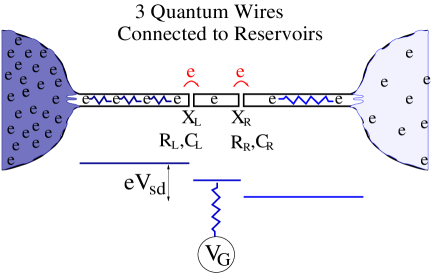
Figure 1: (color online) Model system. Two long wires are adiabatically connected to reservoirs and a short wire is weakly coupled to the two leads. Tunneling resistances at junction points $X_{L}$ and $X_{R}$ are $R_{L/R}$, and the junction capacitances are considered equal $C_{L}=C_{R}$. Quantum dot is capacitively coupled to the gate electrode.

The total Hamiltonian of the system is then given by the sum of the bosonized LL Hamiltonian $\hat{H}_{0}=\hat{H}_{L}+\hat{H}_{D}+\hat{H}_{R}$ accounting for three isolated wire segments labeled by $\ell=(L,D,R)$, and the tunneling Hamiltonian $\hat{H}_{T}$ accounting for single-electron hops through the junctions L and R at $X_{L}$ and $X_{R}$ respectively,

$$\hat{H}=\hat{H}_{0}+\hat{H}_{T}.$$ (2)

Using standard bosonization technique, the Hamiltonian describing each wire segment can be expressed in terms of creation and annihilation operators for collective excitations ($\hat{b}^{\dagger}$ and $\hat{b}$) Voit (1995); Gogolin et al. (1998). For the semi-infinite leads, it reads

$$\hat{H}_{\ell}=\sum_{\nu=1}^{M}\varepsilon^{(\ell)}_{\nu}\sum_{m=1}^{\infty}m\hat{b}^{\dagger}_{\nu,m}\hat{b}_{\nu,m}~{},~{}\mbox{ for }~{}\ell=L,R~{}\,,$$ (3)

where the index $\nu$ labels the $M$ transport sectors of the conductor and $m$ the wave-like collective excitations on each transport sector. The effects of the Coulomb interaction in 1D wire are characterized by the Luttinger parameter $g_{\nu}$: $g=1$ for noninteracting Fermi gas and $0<g<1$ for the repulsive interactions ($g\ll 1$ in the strong interaction limit). The Coulomb interaction also renormalizes the Fermi velocity to $v_{\nu}=v_{F}/g_{\nu}$. The energy of an elementary excitation in sector $\nu$ is given by $\varepsilon_{\nu}=\pi\hbar v_{\nu}/L$ where $L$ is the length of the wire and $\hbar$ the Planck constant. For instance, if the wire has a single transport channel (usually referred to as spinless electrons), e.g. a wire with one transport channel under a strong magnetic field, the system’s dynamics is determined by collective charge excitations (plasmons) alone ($\nu=\rho$ and $M=1$). If, however, the spin degrees of freedom survive, the wire has two transport sectors ($M=2$); plasmons ($\nu=\rho$) and spin-waves ($\nu=\sigma$) Voit (1995). If the system has two transport channels with electrons carrying spin ($M=4$), as is the case with SWNTs, the transport sectors are total-charge-plasmons ($\nu=\rho$), relative-charge-plasmons ($\nu=\Delta\rho$), total-spin-waves ($\nu=\sigma$), and relative-spin-waves ($\nu=\Delta\sigma$) Kane et al. (1997); Egger and Gogolin (1997).

For the short central segment, the zero-mode need to be accounted for as well, which yields

$$\hat{H}_{D}=\sum_{\nu}\varepsilon_{\nu}\sum_{m=1}^{\infty}m\hat{b}^{\dagger}_{\nu,m}\hat{b}_{\nu,m}\\ +\frac{\varepsilon_{\rho}}{2Mg_{\rho}}(\hat{N}_{\rho}-N_{G})^{2}+\sum_{\nu\neq\rho}\frac{\varepsilon_{\nu}}{2Mg_{\nu}}\hat{N}_{\nu}^{2}-E_{r}.$$ (4)

In the second line of Eq. (4), which represents the zero-mode energy of the quantum dot, the operator $\hat{N_{\nu}}$ measures the ground state charge, i.e. with no excitations, in the $\nu$-sector. The zero-mode energy systematically incorporates Coulomb interaction in terms of the Luttinger parameter $g_{\rho}$ in the QD. To refer to the zero-mode energy later in this paper, we define the “charging energy” $E_{C}$ as the minimum energy cost to add an excess electron to the QD in the off-Coulomb blockade regime, i.e.,

$$E_{C}=[E_{D}(2,0)-E_{D}(1,0)]_{N_{G}=1/2}=\varepsilon_{p}/g\,.$$ (5)

Note that this is twice the conventional definition. The charging energy vanishes in the noninteracting limit ($g_{\rho}=1$) and becomes the governing energy scale in the strong interaction limit ($g_{\rho}\ll 1$). The origin of the charging energy in conventional quantum dots is the long range nature of the Coulomb interaction. In the theory of Luttinger liquid, the long range interaction can easily be incorporated microscopically through the interaction strength $g_{\rho}$. For the effect of the finite-range interaction across a tunneling junction, for instance see Refs. Sassetti et al., 1997; Sassetti and Kramer, 1997.

Note that charge and spin are decoupled in Luttinger liquids, which implies the electric forces affect the (total) charge sector only; due to intrinsic $e-e$ interactions, $g_{\rho}<1$ but $g_{\nu\neq\rho}=1$, and the gate voltage shifts the band bottom of the (total) charge sector as seen by the dimensionless gate voltage parameter $N_{G}$ in Eq. (4). As will be shown shortly, the transport properties of the L/R–leads are determined by the LL interaction parameter $g_{\rho}$ and the number of the transport sector $M$. In this work, we consider each wire segment has the same interaction strength for the (total) charge sector, $g\equiv g^{(L)}_{\rho}=g^{(R)}_{\rho}=g^{(D)}_{\rho}$. Accordingly, the energy scales in the quantum dot are written by $\varepsilon_{\rho}\equiv\varepsilon^{(D)}_{\rho}=\pi\hbar v_{F}/g_{\rho}L_{D}$ and $\varepsilon_{0}\equiv\varepsilon_{\nu\neq\rho}=\pi\hbar v_{F}/L_{D}$.

We consider the ground state energy in the QD is the same as those in the leads, by choosing the reference energy $E_{r}$ in Eq. (4) equals the minimum value of the zero-mode energy,

$$E_{r}=\min\left(\frac{\varepsilon_{\rho}N_{G}^{2}}{2Mg_{\rho}},\frac{\varepsilon_{\rho}(1-N_{G})^{2}}{2Mg_{\rho}}+\frac{\varepsilon_{0}(M-1)}{2M}\right),$$ (6)

where $\min(x,x^{\prime})$ denotes the smaller of $x$ and $x^{\prime}$, and the gate charge $N_{G}$ is in the range $N_{G}\in[0,M]$.

The zero-mode energy in the QD,

$$E_{0}=\frac{\varepsilon_{\rho}}{2Mg_{\rho}}(N-N_{G})^{2}+\frac{\varepsilon_{0}}{2M}\sum_{\nu\neq\rho}N_{\nu}^{2}-E_{r}$$ (7)

yields degenerate ground states for $N=0$ and $N=1$ excess electrons when $N_{G}=\big{[}(M-1)g_{\rho}^{2}+1\big{]}/2$. Here we replaced $N_{\rho}$ by the number of the total excess electrons $N$ since $N_{\rho}=N$, and $N_{\nu}$ are all either even or odd integers, simultaneously; in the case of the SWNTs with $N=\sum_{i,s}N_{i,s}$ excess electrons, where $i=1,2$ is the channel index and $s=\uparrow,\downarrow$ is the spin index of conduction electrons (M=4), $N_{\rho}=N$, $N_{\sigma}=\sum_{i}(N_{i,\uparrow}-N_{i,\downarrow})$, $N_{\Delta\rho}=\sum_{s}(N_{1,s}-N_{2,s})$, and $N_{\Delta\sigma}=\sum_{i}(-1)^{i}(N_{i,\uparrow}-N_{i,\downarrow})$.

From now on we consider only one spin-polarized (or spinless) channel unless otherwise stated — our focus is on the role of Coulomb interactions, and the additional channels only lead to more complicated excitation spectra without any qualitative change in the physics we address below. A physical realization of the single-channel case may be obtained e.g by exposing the quantum wire to a large magnetic field.

For the system with high tunneling barriers, the electron transport is determined by the bare electron hops at the tunneling barriers. The tunneling events in the DB structure are described by the Hamiltonian

$$\hat{H}_{T}=\sum_{\ell=L,R}\left[t_{\ell}\hat{\Psi}^{\dagger}_{D}(X_{\ell})\hat{\Psi}_{\ell}(X_{\ell})+H.C.\right],$$ (8)

where $\hat{\Psi}^{\dagger}_{l}(X_{\ell})$ and $\hat{\Psi}_{l}(X_{\ell})$ are the electron creation and annihilation operators at the edges of the wires near the junctions at $X_{L}$ and $X_{R}$. As mentioned earlier, the electron field operators $\hat{\Psi}$ and $\hat{\Psi}^{\dagger}$ are related to the plasmon creation and annihilation operators $b$ and $b^{\dagger}$ by the standard bosonization technique. Different boundary conditions yield different relations between electron field operators and plasmon operators. Exact solutions for the periodic boundary condition have been known for decades Haldane (1981); Voit (1995) but the open boundary conditions which are apt for our system of consideration has been investigated only recently (See for example Refs. Fabrizio and Gogolin, 1995; Eggert et al., 1996; Kane et al., 1997; Mattsson et al., 1997).

The dc bias voltage $V=V_{L}+V_{R}$ between L and R leads is incorporated into the phase factor of the tunneling matrix elements $t_{\ell}=|t_{\ell}|\exp(\mp ieV_{\ell}t/\hbar)$ by a time-dependent unitary transformation Ingold and Nazarov (1992). Here $V_{L/R}=VC/C_{R/L}$ is voltage drop across the L/R–junction where $C=C_{L}C_{R}/(C_{L}+C_{R})$ is the effective total capacitance of the double junction, and the bare tunneling matrix amplitudes $|t_{L/R}|$ are assumed to be energy independent. Experimentally, the tunneling matrix amplitude is sensitive to the junction properties while the capacitance is not. For simplicity, the capacitances are thus assumed to be symmetric $C_{L}=C_{R}$ throughout this work. By junction asymmetry we mean the asymmetry in (bare) squared tunneling amplitudes $|t_{L/R}|^{2}$. The parameter $R=|t_{L}|^{2}/|t_{R}|^{2}$ is used to describe junction asymmetry; $R=1$ for symmetric junctions and $R\gg 1$ for a highly asymmetric junctions.

It is known that, at low energy scales in the quantum wires with the electron density away from half-filling, the processes of backward and Umklapp scattering, whose processes generate momentum transfer across the Fermi sea ($\approx 2k_{F}$), can be safely ignored in the middle of ideal 1D conductors Voit (1995), including armchair SWNTs Kane et al. (1997). The Hamiltonian (2) does not include the backward and Umklapp scattering (except at the tunneling barriers) and therefore it is valid away from half-electron-filling.

We find that, in the regime where electron spin does not play a role, the addition of a transport channel does not change essential physics present in a single transport channel. Therefore, we primarily focus attention to a QW of single transport channel with spinless electrons and will comment on the effects due to multiple channel generalization, if needed.

II.2 Electron transition rates

The occupation probability of the quantum states in the SET system changes via electron tunneling events across L/R–junctions. In the single-electron tunneling regime, the bare tunneling amplitudes $|t_{L/R}|$ are small compared to the characteristic energy scales of the system and the electron tunneling is the source of small perturbation of three isolated LLs. In this regime, we calculate transition rates $\Gamma_{L/R}$ between eigenstates of the unperturbed Hamiltonian $H_{0}$ to the lowest non-vanishing order in the tunneling amplitudes $|t_{L/R}|$. In this golden rule approximation, we integrate out lead degrees of freedom since the leads are in internal equilibria, and the transition rates are given as a function of the state variables and the energies of the QD only Kim et al. (2003); Braggio et al. (2000),

$$\Gamma_{L/R}\left(N^{\prime},\{n^{\prime}\}\leftarrow N,\{n\}\right)\\ =\frac{2\pi}{\hbar}|t_{L/R}|^{2}\,\gamma(W_{L/R})\,\gamma_{D}(\{n^{\prime}\},\{n\})\,.$$ (9)

In Eq. (9) $W_{L/R}$ is the change in the Gibbs free energy associated with the tunneling across the L/R–junction,

$$W_{L/R}=E_{D}(N^{\prime},\{n^{\prime}\})-E_{D}(N,\{n\})\\ \mbox{}\mp(N^{\prime}-N)eV_{L/R}\,.$$ (10)

Here $E_{D}(N,\{n\})=\langle N,\{n\}|\hat{H}_{D}|N,\{n\}\rangle$ is the energy of the eigenstate $|N,\{n\}\rangle$ of the dot and $L/R$ correspond to $-/+$. For the QD with only one transport channel with spinless electrons only,

$$E_{D}(N,\{n\})=\varepsilon_{p}\left[\sum_{m=1}^{\infty}mn_{m}+\frac{(N-N_{G})^{2}}{2g_{D}}\right]-E_{r}\,,$$ (11)

where $\varepsilon_{p}=\varepsilon_{\rho}$ accounting that we consider only charge plasmons and $n_{m}=\langle n_{m}|\hat{b}^{\dagger}_{m}\hat{b}_{m}|n_{m}\rangle$ is the number of plasmons in the mode $m$.

The function $\gamma(x)$ in Eq. (9) is responsible for the plasmon excitations on the leads, and given by (see e.g. Ref. Furusaki, 1998)

$$\gamma(\varepsilon)=\frac{1}{2\pi\hbar}\int_{-\infty}^{\infty}dte^{i\varepsilon t}\langle\Psi_{\ell}(X_{\ell},0)\Psi_{\ell}^{\dagger}(X_{\ell},t)\rangle=\frac{1}{2\pi\hbar}\frac{1}{\pi v_{F}}\left(\frac{2\pi\Lambda g^{1/(1-g)}}{\hbar v_{F}\beta}\right)^{\alpha}\left|\Gamma\left(\frac{1+\alpha}{2}+i\frac{\beta\varepsilon}{2\pi}\right)\right|^{2}\frac{e^{-\beta\varepsilon/2}}{\Gamma(1+\alpha)}\,,$$ (12)

where $\beta=1/k_{B}T$ is the inverse temperature in the leads, $\Lambda$ is a short wavelength cutoff, and $\Gamma(z)$ is the Gamma function. The exponent $\alpha=(g^{-1}-1)/M$ is a characteristic power law exponent indicating interaction strength of the leads with $M$ transport sectors (hence, in our case, $M=1$). At $g=1$ (non-interacting case), the exponent $\alpha=0$ and it grows as $g\to 0$ (strong interaction). The decrease of the exponent $\alpha$ with increasing $M$ implies that the effective interaction decreases due to multi-channel effect, and the Luttinger liquid eventually crosses over to a Fermi liquid in the many transport channel limit Matveev and Glazman (1993a, b).

For the non-interacting electron gas, the spectral density $\gamma(\varepsilon)$ is the TDOS multiplied by the Fermi-Dirac distribution function $f_{FD}(\varepsilon)=[1+\exp(\beta\varepsilon)]^{-1}$; $\gamma(\varepsilon)=\frac{1}{\pi\hbar v_{F}}f_{FD}(\varepsilon)$ for $g=1$. At zero temperature, $\gamma(\varepsilon)$ is proportional to a power of energy,

$$\lim_{T\rightarrow 0}\gamma(\varepsilon)=\Theta(-\varepsilon)\frac{1}{\pi\hbar v_{F}}\frac{\left(|\varepsilon|/\varepsilon_{\Lambda}\right)^{\alpha}}{\Gamma(\alpha+1)},$$ (13)

where $\varepsilon_{\Lambda}=\hbar v_{F}/\Lambda g^{1/(1-g)}$ is a high energy cut-off. At zero temperature $\gamma(\varepsilon)$ is the TDOS for the negative energies and zero otherwise (as it should be), imposed by the unit step function $\Theta(-\varepsilon)$.

The function $\gamma_{D}$ in Eq. (9) accounts for the plasmon transition amplitudes in the QD, and is given by

$$\gamma_{D}(\{n^{\prime}\},\{n\})=\delta_{N^{\prime},N+1}|\langle N^{\prime},\{n^{\prime}\}|\hat{\Psi}^{\dagger}_{D}(X_{\ell})|N,\{n\}\rangle|^{2}\\ +\delta_{N^{\prime},N-1}|\langle N^{\prime},\{n^{\prime}\}|\hat{\Psi}_{D}(X_{\ell})|N,\{n\}\rangle|^{2}$$ (14)

where we used that the zero-mode overlap is unity for $N^{\prime}=N\pm 1$ and vanishes otherwise. The overlap integrals between plasmon modes are, although straightforward, quite tedious to calculate, and we refer to Appendix A for the details. The resulting overlap of the plasmon states can be written as a function of the mode occupations $n_{m}$,

$$|\langle\{n^{\prime}\}|\hat{\Psi}^{\dagger}_{D}(X_{\ell})|\{n\}\rangle|^{2}=|\langle\{n^{\prime}\}|\hat{\Psi}_{D}(X_{\ell})|\{n\}\rangle|^{2}\\ =\frac{1}{L_{D}}\left(\frac{\pi\Lambda}{L_{D}}\right)^{\alpha_{D}}\phi(\{n^{\prime}\},\{n\})$$ (15)

with

$$\phi(\{n^{\prime}\},\{n\})\\ =\prod_{m=1}^{\infty}\left(\frac{1}{gm}\right)^{|n^{\prime}_{m}-n_{m}|}\frac{n_{m}^{(<)}!}{n^{(>)}_{m}!}\left[L^{|n_{m}^{\prime}-n_{m}|}_{n_{m}^{(<)}}\left(\frac{1}{gm}\right)\right]^{2}$$ (16)

where $n_{m}^{(<)}=\min(n_{m}^{\prime},n_{m})$ and $n_{m}^{(>)}=\max(n_{m}^{\prime},n_{m})$, $\alpha_{D}=(g_{D}^{-1}-1)$ for the QD with one transport sector, and $L_{a}^{b}(x)$ are Laguerre polynomials. Additional transport sectors would appear as multiplicative factors of the same form as $\phi(\{n^{\prime}\},\{n\})$ and result in a reduction of the exponent $\alpha_{D}$. Notice that in the low energy scale only the first few occupations $n_{m}$ and $n^{\prime}_{m}$ in the product differ from zero, participating to the transition rate (9) with nontrivial contributions.

II.3 Plasmon relaxation process in the quantum dot

In general, plasmons on the dot are excited by tunneling events and have a highly non-equilibrium distribution. The coupling of the system to the environment such as external circuit or background charge in the substrate leads to relaxation towards the equilibrium. While the precise form of the relaxation rate, $\Gamma_{p}$, depends on the details of the relaxation mechanism, the physical properties of our concern do not depend on the details. Here we take a phenomenological model where the plasmons are coupled to a bath of harmonic oscillators by

$$H_{\mathrm{plasmon-bath}}=\sum_{m,n}\sum_{\alpha}\left(g_{mn}^{\alpha}\,b_{m}^{\dagger}b_{n}a_{\alpha}+h.c.\right)\,.$$ (17)

In Eq. (17) $a_{\alpha}$ and $a_{\alpha}^{\dagger}$ are bosonic operators describing the oscillator bath and $g_{mn}^{\alpha}$ is the coupling constants. We will assume an Ohmic form of the bath spectral density function

$$J_{mn}(\omega)\equiv\sum_{\alpha}|g_{mn}^{\alpha}|^{2}\,\delta(\omega-\omega_{\alpha})=\gamma_{p}\Gamma_{0}\omega\,,$$ (18)

where $\omega_{\alpha}$ is the frequency of the oscillator corresponding to $a_{\alpha}$, $\gamma_{p}$ is a dimensionless constant characterizing the bath spectral density, and $\Gamma_{0}^{-1}=\hbar^{2}v_{F}L_{D}(|t_{L}|^{-2}+|t_{R}|^{-2})$ is the natural time scale of the system. Within the rotating-wave approximation, the plasmon transition rate due to the harmonic oscillator bath is given by

$$\Gamma_{p}(\{n^{\prime}\}\leftarrow\{n\})=\gamma_{p}\Gamma_{0}\frac{W_{p}/\varepsilon_{p}}{e^{\beta W_{p}}-1}$$ (19)

with $W_{p}=\varepsilon_{p}\sum_{m}(n_{m}^{\prime}-n_{m})$, where $\varepsilon_{p}=\varepsilon_{\rho}$ is the plasmon energy. Note that these phenomenological rates obey detailed balance and, therefore, at low temperatures only processes that reduce the total plasmon energy occur with appreciable rates.

II.4 Matrix formulation

For later convenience, we introduce a matrix notation for the transition rates $\Gamma$, with the matrix elements defined by

$$\left[\widehat{\mathbf{\textstyle\Gamma}}_{\ell}^{\pm}(N)\right]_{\{n^{\prime}\},\{n\}}=\Gamma_{\ell}(N\pm 1,\left\{\textstyle n^{\prime}\right\}\leftarrow N,\left\{\textstyle n\right\})\,,$$ (20)

i.e, the element $(\{n^{\prime}\},\{n\})$ of the matrix block $\widehat{\mathbf{\textstyle\Gamma}}_{\ell}^{\pm}(N)$ is the transition rate $\Gamma_{\ell}(N\pm 1,\left\{\textstyle n^{\prime}\right\}\leftarrow N,\left\{\textstyle n\right\})$. Similarly,

$$\left[\widehat{\mathbf{\textstyle\Gamma}}_{\ell}^{0}\right]_{\{n^{\prime}\},\{n\}}\\ \mbox{}=\delta_{\{n^{\prime}\},\{n\}}\sum_{\{n^{\prime\prime}\}}\left[\widehat{\mathbf{\textstyle\Gamma}}_{\ell}^{+}+\widehat{\mathbf{\textstyle\Gamma}}_{\ell}^{-}\right]_{\{n^{\prime\prime}\},\{n\}}\,,$$ (21)

and

$$\left[\widehat{\mathbf{\textstyle\Gamma}}_{p}(N)\right]_{\{n^{\prime}\},\{n\}}=-\Gamma_{p}(\left\{\textstyle n^{\prime}\right\},\left\{\textstyle n\right\})\\ \mbox{}+\delta_{\{n^{\prime}\},\{n\}}\sum_{\{n^{\prime\prime}\}}\Gamma_{p}(\left\{\textstyle n^{\prime\prime}\right\},\left\{\textstyle n\right\})\,.$$ (22)

Master equation (1) can now be conveniently expressed as

$$\frac{d}{dt}\left|\textstyle P(t)\right\rangle=-\widehat{\mathbf{\textstyle\Gamma}}\left|\textstyle P(t)\right\rangle$$ (23)

with $\widehat{\mathbf{\textstyle\Gamma}}=\widehat{\mathbf{\textstyle\Gamma}}_{p}+\sum_{\ell=L,R}\left(\widehat{\mathbf{\textstyle\Gamma}}_{\ell}^{0}-\widehat{\mathbf{\textstyle\Gamma}}_{\ell}^{+}-\widehat{\mathbf{\textstyle\Gamma}}_{\ell}^{-}\right)$, where $\left|\textstyle P(t)\right\rangle$ is the column vector (not to be confused with the “ket” in quantum mechanics) with elements given by $\left\langle\textstyle N,\left\{\textstyle n\right\}|P(t)\right\rangle\equiv P(N,\left\{\textstyle n\right\},t)$. Therefore, the time evolution of the probability vector satisfies

$$\left|\textstyle P(t)\right\rangle=\exp(-\widehat{\mathbf{\textstyle\Gamma}}t)\left|\textstyle P(0)\right\rangle.$$ (24)

In the long time limit, the system reaches a steady state $\left|\textstyle P(\infty)\right\rangle$.

The ensemble averages of the matrices $\widehat{\mathbf{\textstyle\Gamma}}^{\pm}_{\ell}$ can then be defined by

$$\left\langle\textstyle\widehat{\mathbf{\textstyle\Gamma}}^{\pm}_{\ell}(t)\right\rangle=\sum_{N,\{n\}}\left\langle\textstyle N,\{n\}\right|\widehat{\mathbf{\textstyle\Gamma}}^{\pm}_{\ell}\left|\textstyle P(t)\right\rangle\,.$$ (25)

We will construct other statistical quantities such as average current and noise power density based on Eq. (25).

III Steady-state probability distribution of nonequilibrium plasmons

By solving the master equation (23) numerically (without plasmon relaxation), in Ref. Kim et al., 2003, we obtained the occupation probabilities of the plasmonic many-body excitations as a function of the bias voltage and the interaction strength. We found that in the weak to noninteracting regime, $\alpha\approx 0$ or $g=1/(1+\alpha)\approx 1$ for the wire with one transport sector, the non-equilibrium probability of plasmon excitations is a complicated function of the detailed configuration of state occupations $\{n\}=(n_{1},n_{2},\cdots,n_{m},\cdots)$.

In contrast, the non-equilibrium occupation probability in the strong interaction regime with (nearly) symmetric tunneling barriers depends only on the total energy of the states, and follows a universal form irrespective of electron charge $N$ in the QD. In the leading order approximation, it is given by

$$P^{(0)}(\varepsilon)\approx\frac{1}{Z}\exp\left(-\frac{3(\alpha+1)}{2}\frac{\varepsilon}{eV}\log\frac{\varepsilon}{\varepsilon_{p}}\right),$$ (26)

where $Z$ is a normalization constant. Notice that $\varepsilon$ is the total energy, including zero-mode and plasmon contributions. The distribution has a universal form which depends on the bias voltage and the interaction strength. The detailed derivation is in appendix B. This analytic form is valid for the not too low energies $(\varepsilon,eV)\gtrsim 3\varepsilon_{p}$ and in the strongly interacting regime $\alpha\gtrsim 1$. More accurate approximation formula (Eq. (94)) is derived in appendix B.

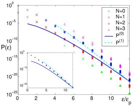
(a)

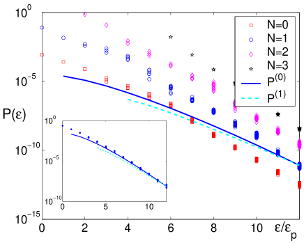
(b)

Figure 2: (color online) The occupation probability $P(\varepsilon)$ as a function of the mode energy $\varepsilon/\varepsilon_{p}$. The energy $\varepsilon$ is abbreviation for $E_{D}(N,\{n\})$, the bias $eV=6\varepsilon_{p}$, the asymmetry parameter $R=100$, and $N_{G}=1/2$ ($T=0$). Two analytic approximations, Eq. (26) (blue curve) and Eq. (94) (cyan curve), are fitted to the probability distribution of the charge mode $N=1$ (blue circle). The interaction parameter is (a) $g=0.2$ and (b) $g=0.5$. In the inset the case of symmetric junctions ($R=1$) is plotted with the same conditions.

For symmetric junctions, the occupation probabilities fall on a single curve, well approximated by the analytic formulas Eqs. (26) and (94), as seen in the insets in Fig. 2, where $P(\varepsilon)$ is depicted as a function of the state energies for (a) $g=0.2$ and (b) $g=0.5$, with parameters $R=1$ for the inset and $R=100$ for the main figures ($eV=6\varepsilon_{p}$, $N_{G}=1/2$). For the asymmetric junctions, the line splits into several branches, one for each electric charge $N$, see the figure. However, as seen in 2(a), if the interaction is strong enough ($g\lesssim 0.3$ for $R=100$ and $eV=6\varepsilon_{p}$), each branch is, independently, well described by Eq. (26) or (94). For weaker interactions, $g\gtrsim 0.3$ for $R=100$ and $eV=6\varepsilon_{p}$, the analytic approximation is considerably less accurate as shown in 2(b). Even in the case of weaker interactions, however, the logarithms of the plasmon occupation probabilities continue to be nearly linear in $\varepsilon$ but with a slope that deviates from that seen for symmetric junctions.

IV Average current

In terms of the tunneling current matrices $\hat{\mathbf{\textstyle I}}_{L/R}$ across the junction $L/R$

$$\hat{\mathbf{\textstyle I}}_{L/R}=\mp e\left(\widehat{\mathbf{\textstyle\Gamma}}_{L/R}^{+}-\widehat{\mathbf{\textstyle\Gamma}}_{L/R}^{-}\right),$$ (27)

the average current $I_{L/R}(t)=\left\langle\textstyle\hat{\mathbf{\textstyle I}}_{L/R}(t)\right\rangle$ through $L/R$–junction is

$$I_{L/R}(t)=\sum_{N,\{n\}}\left\langle\textstyle N,\{n\}\right|\hat{\mathbf{\textstyle I}}_{L/R}\left|\textstyle P(t)\right\rangle.$$ (28)

The total external current $I(t)=\left\langle\textstyle\hat{\mathbf{\textstyle I}}(t)\right\rangle$, which includes the displacement currents associated with charging and discharging the capacitors at the left and right tunnel junctions, is then conveniently written as

$$I(t)=\sum_{\ell=L,R}(C/C_{\ell})I_{\ell}(t),$$ (29)

where $C^{-1}=C_{L}^{-1}+C_{R}^{-1}$. As the system reaches steady-state in the long time limit, the charge current is conserved throughout the system, $I=I(\infty)=I_{L}(\infty)=I_{R}(\infty)$.

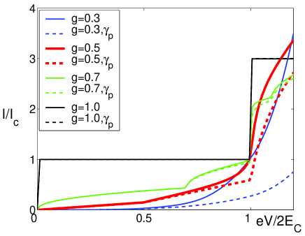
Figure 3: (color online) Average current $I/I_{c}$ as a function of the bias voltage $eV/2E_{C}$ and LL interaction parameter $g$ (black line for $g=1$, green $g=0.7$, red $g=0.5$, blue $g=0.3$, respectively) for $R=100$ (highly asymmetric junctions) with no plasmon relaxation ($\gamma_{p}=0$, solid lines) or with fast plasmon relaxation ($\gamma_{0}=10^{4}$, dashed lines). The bias voltage is normalized by the charging energy $2E_{C}$ and current is normalized by the current at $eV=2E_{C}$ with no plasmon relaxation for each $g$. Other parameters are $N_{G}=1/2$, $T=0$.

One consequence of non-equilibrium plasmons is the increase in current as shown in Fig. 3, where the average current is shown as a function of the bias for different interaction strengths. The currents are normalized by $I_{c}=I(eV=2E_{C})$ with no plasmon relaxation ($\gamma_{p}=0$) for each interaction strength $g$, and we see that the current enhancement is substantial in the strong interaction regime ($g\lesssim 0.5$), while there is effectively no enhancement in noninteracting limit $g=1$ (the two black lines are indistinguishable in the figure). In the weak interaction limit the current increases in discrete steps as new transport channels become energetically allowed, while at stronger interactions the steps are smeared to power laws with exponents that depend on the number of the plasmon states involved in the transport processes.

Including the spin sector results in additional peaks in the average current voltage characteristic that can be controlled by the transverse magnetic field Braggio et al. (2001); Cavaliere et al. (2004).

The current-voltage characteristics show that, in the non-interaction limit, the non-equilibrium approach predicts similar behavior for the average current as the detailed balance approach which assumes thermal equilibrium in the QD. In contrast, in the strong interaction regime, non-equilibrium effects give rise to an enhancement of the particle current.

Experimentally, however, the current enhancement may be difficult to attribute to plasmon distribution as the current levels depend on barrier transparencies and plasmon relaxation rates, and neither of them can be easily tuned. We now turn to another experimental probe, the shot noise, which is more sensitive to non-equilibrium effects.

V Current noise

Noise in electronic conductors is given by the ensemble average of the current-current correlations Kogan (1996); Beenakker and Schönenberger (2003). Thermal fluctuations and the discrete nature of the electron charge are two fundamental sources of the noise; in specific devices there may additional noise sources due to, e.g., fluctuating environmental variables. Thermal (equilibrium) noise is not very informative since it does not provide more information than the equilibrium conductance of the system. In contrast, shot noise, which is a consequence of the discreteness of charge and the stochastic nature of transport, can provide further insight beyond average current since it is a sensitive function of the correlation mechanism, internal excitations, and the statistics of the charge carriers de Jong and Beenakker (1997); Blanter and Büttiker (2000).

Influence of quantum coherence on shot noise is an intriguing issue. It is known that the ensemble averaged quantum mechanical calculations of shot noise to the leading order is identical to the semiclassical approaches when the comparable theories are available (Blanter and Büttiker, 2000, in Sec. 5). However, the word “semiclassical” should not be confused with the deterministic motion of the transport charges. For instance, Oberholzer et al. (2002) discuss the crossover from full quantum to classical shot noise, by tuning the electron dwell time in chaotic cavities, where by classical it means the deterministic nature of electron motion.

Shot noise in interacting one-dimensional systems has also been the subject of many recent works. For instance, the shot noise of the edge states was used to measure the factional charge $ge$ of the quasiparticles in the fractional quantum Hall states Kane and Fisher (1994); Saminadayar et al. (1997); de Picciotto et al. (1997); Comforti et al. (2002).

The shot noise of double-barrier structures was widely studied in the last decade. In conventional SET structures, shot noise is suppressed below the Poisson limit due to the Coulomb correlations (in addition to the Fermi correlation): the $e-e$ correlations typically result in reduction of shot noise. Both quantum mechanical approaches Chen and Ting (1991); Bøand Galperin (1996) and semiclassical derivations based on a master equation approach predict identical shot noise results Davies et al. (1992); Chen and Ting (1992); Chen (1993), implying that the shot noise is not sensitive to the quantum coherence in DB structures. If the leads are superconducting in the SET structure, the tunneling particles are either single-electrons or Cooper-pairs and the shot noise is a functional of the dephasing process of the Cooper-pairs Deblock et al. (2003); Choi et al. (2001, 2003).

Semiclassical theories of shot noise based on a master equation approach in the sequential tunneling regime for a SET have been developed by many authors Davies et al. (1992); Hershfield et al. (1993); Chen and Ting (1992); Korotkov et al. (1992); Korotkov (1994); Hanke et al. (1994). The predictions of some of these theories Hershfield et al. (1993) have been experimentally confirmed Birk et al. (1995).

The noise power density in the steady state is given by

$$S(\omega)=\lim_{t\to\infty}2\int_{-\infty}^{\infty}{d\tau}\;e^{+i\omega\tau}\left[\left\langle\textstyle\hat{\mathbf{\textstyle I}}(t+\tau)\hat{\mathbf{\textstyle I}}(t)\right\rangle-\left\langle\textstyle\hat{\mathbf{\textstyle I}}(t)\right\rangle^{2}\right]\,.$$ (30)

The correlation functions $K_{\ell\ell^{\prime}}(\tau)=\lim_{t\to\infty}\left\langle\textstyle\hat{\mathbf{\textstyle I}}_{\ell}(t+\tau)\hat{\mathbf{\textstyle I}}_{\ell^{\prime}}(t)\right\rangle$ can be deduced from the master equation (23). In the matrix notation they can be written as Hershfield et al. (1993); Korotkov (1994)

$$K_{\ell\ell^{\prime}}(\tau)=e^{2}\sum_{N,\left\{\textstyle n\right\}}\left\langle\textstyle N,\left\{\textstyle n\right\}\right|\Bigg{[}\Theta(+\tau)\hat{\mathbf{\textstyle I}}_{\ell}\exp(-\widehat{\mathbf{\textstyle\Gamma}}\tau)\hat{\mathbf{\textstyle I}}_{\ell^{\prime}}\\ \mbox{}+\Theta(-\tau)\hat{\mathbf{\textstyle I}}_{\ell^{\prime}}\exp(+\widehat{\mathbf{\textstyle\Gamma}}\tau)\hat{\mathbf{\textstyle I}}_{\ell}\\ \mbox{}+\delta(\tau)\delta_{\ell\ell^{\prime}}\left(\widehat{\mathbf{\textstyle\Gamma}}_{\ell}^{+}+\widehat{\mathbf{\textstyle\Gamma}}_{\ell}^{-}\right)\Bigg{]}\left|\textstyle P(\infty)\right\rangle\,,$$ (31)

where $\Theta(x)$ is the unit step function.

To investigate the correlation effects, the noise power customarily compared to the Poisson value $S_{Poisson}=2eI$. The Fano factor is defined as the ratio of the actual noise power and the Poisson value,

$$F\equiv\frac{S(0)}{2eI}.$$ (32)

Since thermal noise ($S=4k_{B}TG(V=0)$) is not particularly interesting, we focus on the zero frequency shot noise, in the low bias voltage regime where the Coulomb blockade governs the electric transport; $T=0$ and $eV\lesssim 2E_{C}$.

We begin by considering analytically tractable cases with only a few involved states, and then proceed to the full numerical results. The finite frequency shot noise is briefly discussed in subsection V.5.

V.1 Two-state model; $eV\approx\varepsilon_{p}$

The electron transport involving only two lowest energy states in the quantum dot are well studied by many authors (see, for instance, Ref. Blanter and Büttiker, 2000). Nevertheless, for later reference we begin the discussion of shot noise with two-state process, which provides a reasonable approximation for $eV\approx\varepsilon_{p}$. At biases such that $eV\approx\varepsilon_{p}$ and sufficiently low temperatures, the two lowest states $\left|\textstyle N,n_{1}\right\rangle=\left|\textstyle 0,0\right\rangle$ and $\left|\textstyle 1,0\right\rangle$ dominate the transport process and the rate matrix is given by

$$\widehat{\mathbf{\textstyle\Gamma}}=\left[\begin{array}[]{cc}\gamma^{+}&-\gamma^{-}\\ -\gamma^{+}&\gamma^{-}\end{array}\right]~{},$$ (33)

where the matrix elements are $\gamma^{+}\equiv\Gamma_{L}(1,0\leftarrow 0,0)$ and $\gamma^{-}\equiv\Gamma_{R}(0,0\leftarrow 1,0)$.

With the current matrices defined by Eq. (27)

$$\hat{\mathbf{\textstyle I}}_{L}=\left[\begin{array}[]{cc}0&0\\ \gamma^{+}&0\end{array}\right]~{},~{}~{}\hat{\mathbf{\textstyle I}}_{R}=\left[\begin{array}[]{cc}0&\gamma^{-}\\ 0&0\end{array}\right]~{},$$

the noise power is obtained straightforwardly by Eqs. (30) and (31) using the steady state probability

$$\left|\textstyle P(\infty)\right\rangle=\left[\begin{array}[]{c}P_{00}\\ P_{10}\end{array}\right]=\frac{1}{\gamma^{+}+\gamma^{-}}\left[\begin{array}[]{c}\gamma^{-}\\ \gamma^{+}\end{array}\right].$$ (34)

The Fano factor (32) takes a simple form

$$F_{2}=P_{00}^{2}+P_{10}^{2}=\frac{1+(\gamma^{-}/\gamma^{+})^{2}}{(1+\gamma^{-}/\gamma^{+})^{2}}$$ (35)

where

$$\frac{\gamma^{-}}{\gamma^{+}}=\frac{1}{R}\left(\frac{eV/2-\delta E_{0}}{eV/2+\delta E_{0}}\right)^{\alpha}$$

and $\delta E_{0}$ is the shift of the bottom of the zero mode energy induced by the gate voltage,

$$\delta E_{0}=(\delta N_{G})\varepsilon_{p}/g,~{}\delta N_{G}=N_{G}-1/2.$$ (36)

Note that Eq. (35) is valid for $|\delta E_{0}|\leq eV/2$, otherwise $I=0$ and $S=0$ due to Coulomb blockade. We see from Eq. (35) that the Fano factor is minimized for $\gamma^{-}/\gamma^{+}=1$ and maximized for $(\gamma^{-}/\gamma^{+})^{\pm 1}=0$, with the bounds $1/2\leq F_{2}<1$. At the gate charge $N_{G}=1/2$, it is determined only by the junction asymmetry parameter $R$: $F_{2}=(1+R^{2})/(1+R)^{2}$. Note that when only two states are involved in the current carrying process (ground state to ground state transitions), the Fano factor cannot exceed the Poisson value $F=1$.

As a consequence of the power law dependence of the transition rates on the transfer energy (13), the Fano factor is a function of the bias voltage, gate voltage, and the interaction strength; it varies between the minimum and maximum values

$$F_{2}=\left\{\begin{array}[]{ll}\displaystyle\frac{1}{2},&~{}\mbox{ at }~{}\displaystyle\delta E_{0}=\frac{1-R^{1/\alpha}}{1+R^{1/\alpha}}\frac{eV}{2}{}\\ 1,&~{}\mbox{ at }~{}\displaystyle\delta E_{0}=\pm\frac{eV}{2}{}\end{array}\right.,$$ (37)

(cf. Eq. (5) in Ref. Braggio et al., 2003).

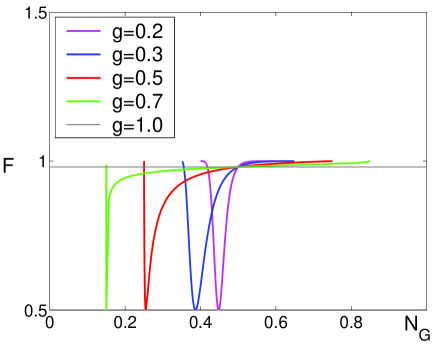
Figure 4: (color online) Fano factor $F\equiv S(0)/2eI$ as a function of the gate charge $N_{G}$ and LL interaction parameter $g$ (black line for $g=1$, green $g=0.7$, red $g=0.5$, blue $g=0.3$, magenta $g=0.2$, respectively) for $R=100$ (highly asymmetric junctions) at $eV=\varepsilon_{p}$ ($T=0$).

Fig. 4 depicts the Fano factor as a function of gate charge $N_{G}$ and interaction parameter $g$ at the bias $eV=\varepsilon_{p}$ for strongly asymmetric junctions $R=100$ ($T=0$). The gate charge $N_{G}$ corresponding to the minimum of the Fano factor ($F=1/2$) in the figure is

$$N_{G}^{\mathrm{dip}}=1/2+g(eV/2\varepsilon_{p})\frac{1-R^{1/\alpha}}{1+R^{1/\alpha}}.$$ (38)

The Fano factor independently of the interaction strength crosses $F_{2}=(1+R^{2})/(1+R)^{2}$ at $N_{G}=1/2$, and it approaches maximum $F_{2}=1$ at $N_{G}=1/2\pm g(eV/2\varepsilon_{p})$. i

V.2 Three-state model; $eV\gtrsim 2\varepsilon_{p}$

The two-state model is applicable for bias voltages below $eV_{\mathrm{th}}=2(\varepsilon_{p}-|\delta E_{0}|)$, since at least three states can be involved in transport above this threshold voltage. For electron transport involving three lowest energy states in the quantum dot, $\left|\textstyle N,n_{1}\right\rangle=\left|\textstyle 0,0\right\rangle,\left|\textstyle 1,0\right\rangle,$ and $\left|\textstyle 1,1\right\rangle$ with $n_{m}=0$ for $m\geq 2$, the noise power can be calculated exactly if the the contribution from the (backward) transitions against the bias is negligible, as is typically the case at zero temperature. In practice, however, the backward transitions are not completely blocked for the bias above the threshold voltage of the plasmon excitations, even at zero temperature: once the bias voltage reaches the threshold to initiate plasmon excitations, the high energy plasmons in the QD above the Fermi energies of the leads are also partially populated, opening the possibility of backward transitions.

A qualitatively new feature that can be studied in the three-state model as compared to the two-state model is plasmon relaxation: the system with a constant total charge may undergo transitions between different plasmon configurations.

We will show in this subsection that the analytic solution of the Fano factor of the three-state process yields an excellent agreement with the low bias numerical results in the strong interaction regime, while it shows small discrepancy in the weak interaction regime (due to non-negligible contribution from the high energy plasmons). We will also show that within the three state model the Fano factor may exceed the Poisson value.

V.2.1 Analytic results

By allowing plasmon relaxation, the rate matrix involving three lowest energy states $\left|\textstyle N,n_{1}\right\rangle=\left|\textstyle 0,0\right\rangle,\left|\textstyle 1,0\right\rangle,$ and $\left|\textstyle 1,1\right\rangle$ is given by

$$\widehat{\mathbf{\textstyle\Gamma}}=\left[\begin{array}[]{ccc}\gamma_{0}^{+}+\gamma_{1}^{+}&-\gamma_{0}^{-}&-\gamma_{1}^{-}\\ -\gamma_{0}^{+}&\gamma_{0}^{-}&-\gamma_{p}\\ -\gamma_{1}^{+}&0&\gamma_{1}^{-}+\gamma_{p}\end{array}\right]~{},$$ (39)

with the matrix elements $\gamma_{i}^{+}\equiv\Gamma_{L}(1,i\leftarrow 0,0),\gamma_{i}^{-}\equiv\Gamma_{R}(0,0\leftarrow 1,i),~{}i=0,1$ and $\gamma_{p}$ introduced in Eq. (19). Current matrices defined by Eq. (27) are

$$[\hat{\mathbf{\textstyle I}}_{L}]_{\{2,1\}}=\gamma_{0}^{+},[\hat{\mathbf{\textstyle I}}_{L}]_{\{3,1\}}=\gamma_{1}^{+},[\hat{\mathbf{\textstyle I}}_{R}]_{\{1,2\}}=\gamma_{0}^{-},[\hat{\mathbf{\textstyle I}}_{R}]_{\{1,3\}}=\gamma_{1}^{-}~{},$$

with $[\hat{\mathbf{\textstyle I}}_{\ell}]_{\{i,j\}}=0$ for other set of $i,j=1,2,3$, where $\ell=L,R$. The noise power is obtained straightforwardly by Eqs. (30) and (31) using the steady state probability

$$\left|\textstyle P(\infty)\right\rangle=\left[\begin{array}[]{c}P_{00}\\ P_{10}\\ P_{11}\end{array}\right]=\frac{1}{Z}\left[\begin{array}[]{c}\gamma_{0}^{-}(\gamma_{1}^{-}+\gamma_{p})\\ \gamma_{0}^{+}(\gamma_{1}^{-}+\gamma_{p})+\gamma_{1}^{+}\gamma_{p}\\ \gamma_{1}^{+}\gamma_{0}^{-}\end{array}\right],$$ (40)

with normalization constant $Z=\gamma_{0}^{+}\gamma_{1}^{-}+\gamma_{1}^{+}\gamma_{0}^{-}+\gamma_{0}^{-}\gamma_{1}^{-}+(\gamma_{0}^{+}+\gamma_{0}^{-}+\gamma_{1}^{+})\gamma_{p}$. Using the average current $I=e(P_{10}\gamma_{0}^{-}+P_{11}\gamma_{1}^{-})$, the Fano factor $F=S(0)/2eI$ is given by

$$F_{3}=P_{00}^{2}+P_{10}^{2}+P_{11}^{2}+2P_{11}\frac{1}{Z}\frac{\gamma_{0}^{+}}{\gamma_{0}^{-}}\\ \times\bigg{[}(\gamma_{0}^{-})^{2}+(\gamma_{1}^{-})^{2}-\gamma_{0}^{-}\gamma_{1}^{-}+\frac{\gamma_{0}^{+}+\gamma_{1}^{+}}{\gamma_{0}^{+}}\gamma_{1}^{-}\gamma_{p}\bigg{]}~{}.$$ (41)

Compared to the Fano factor (35) in the two-state process, complication arises already in the three-state process due to the last term in Eq. (41) which results from the coupling of $P_{11}$ and the rates which cannot be expressed by the components of the probability vector.

In order to have $\left|\textstyle N,n_{1}\right\rangle=\left|\textstyle 0,0\right\rangle,\left|\textstyle 1,0\right\rangle,$ and $\left|\textstyle 1,1\right\rangle$ as the relevant states, we assume $\gamma_{0}^{+}>\gamma_{0}^{-}$ or more explicitly $N_{G}\geq N_{G}^{\mathrm{dip}}$ which is introduced in Eq. (38) . In the opposite situation ($\gamma_{0}^{+}<\gamma_{0}^{-}$), the relevant states are $\left|\textstyle N,n_{1}\right\rangle=\left|\textstyle 0,0\right\rangle,\left|\textstyle 0,1\right\rangle,$ and $\left|\textstyle 1,0\right\rangle$, and above description is still valid with the exchange of electron number $N=0\leftrightarrow 1$ and the corresponding notations $\gamma_{i}^{+}\leftrightarrow\gamma_{i}^{-},~{}i=0,1$.

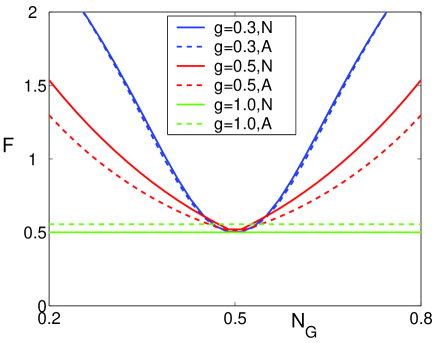
Figure 5: (color online) Fano factor $F\equiv S(0)/2eI$ as a function of the gate charge $N_{G}$ for symmetric junctions ($R=1$) at voltage $eV=2\varepsilon_{p}$ ($T=0$), with no plasmon relaxation. Numerical results (solid lines) vs. analytic results with three states, Eq. (41) (dashed lines) for $g=0.3$ (blue), $0.5$ (red), and $1.0$ (green).

To see the implications of Eq. (41), we plot the Fano factor in Fig. 5, with respect to the gate charge $N_{G}$ for symmetric junctions at $eV=2\varepsilon_{p}$ ($T=0$), with no plasmon relaxation ($\gamma_{p}=0)$.

Two main features are seen in Fig. 5. Firstly, the shot noise is enhanced over the Poisson limit ($F=1$) in the strong interaction regime, $g\lesssim 0.5$, for a range of parameters with gate charges near (but not including) $N_{G}=1/2$. As discussed above, in the low bias regime $eV<2(\varepsilon_{p}-|\delta E_{0}|)$ at zero temperature, no plasmons are excited and the electric charges are transported via only the two-state process following the Fano factor (35) which results in the sub-Poissonian shot noise ($1/2\leq F\leq 1$). Once the bias reaches the threshold $eV_{\mathrm{th}}=2(\varepsilon_{p}-|\delta E_{0}|)$, it initiates plasmon excitations which enhance the shot noise over the Poisson limit. This feature is discussed in more detail below.

Secondly, in the weak interaction regime ($g\gtrsim 0.5$) a small discrepancy between the analytic result (41) (dashed line) and the numerical result (solid line) is found. It results from the partially populated states of the high energy plasmons over the bias due to non-vanishing transition rates. On the other hand, a simple three-state approximation shows excellent agreement in the strong interaction regime ($g=0.3$ in the figure), indicating negligible contribution of the high energy plasmons ($E_{D}(N,\{n\})>eV/2$) to the charge transport mechanism. This is due to the power law suppression of the transition rates (13) as a function of the transfer energy (10).

V.2.2 Limiting cases

To verify the role of non-equilibrium plasmons as the cause of the shot noise enhancement, we consider two limiting cases of Eq. (41): $\gamma_{p}=0$ and $\gamma_{p}\gg\gamma_{i}^{\pm}$.

In the limit of no plasmon relaxation ($\gamma_{p}=0$), the Fano factor (41) of the three-state process is simplified as

$$F_{3}^{(0)}=1-2[(1-P_{10})P_{10}+(1-P_{11})P_{11}]\\ +2P_{10}P_{11}\frac{(\gamma_{0}^{-})^{2}+(\gamma_{1}^{-})^{2}}{\gamma_{0}^{-}\gamma_{1}^{-}},$$ (42)

with steady-state probability

$$\left|\textstyle P(\infty)\right\rangle=\left[\begin{array}[]{c}P_{00}\\ P_{10}\\ P_{11}\end{array}\right]=\frac{1}{Z}\left[\begin{array}[]{c}\gamma_{0}^{-}\gamma_{1}^{-}\\ \gamma_{0}^{+}\gamma_{1}^{-}\\ \gamma_{1}^{+}\gamma_{0}^{-}\end{array}\right],$$ (43)

where the new normalization constant is $Z=\gamma_{0}^{+}\gamma_{1}^{-}+\gamma_{1}^{+}\gamma_{0}^{-}+\gamma_{0}^{-}\gamma_{1}^{-}$.

The three-state approximation is most accurate in the low bias regime $2(\varepsilon_{p}-|\delta E_{0}|)\lesssim eV\ll 2E_{C}$ ($\delta E_{0}$ is defined in Eq. (36)) and for gate voltages away from $N_{G}=1/2$, i.e., for $1/2<N_{G}\lesssim 1$ (or $0\lesssim N_{G}<1/2$ with the exchange of indices regarding particle number $N=0\leftrightarrow 1$). In this regime, $\gamma_{0}^{+}$ and/or $\gamma_{1}^{-}$ dominate over the other rates, ($\gamma_{0}^{+},\gamma_{1}^{-})\gg(\gamma_{0}^{-},\gamma_{1}^{+}$), which results in $1\gtrsim P_{10}\gg(P_{0},P_{11})\approx 0$. The Fano factor (42) now reduces to

$$F_{3}^{(0)}\approx 1+2P_{10}P_{11}\frac{(\gamma_{0}^{-})^{2}+(\gamma_{1}^{-})^{2}}{\gamma_{0}^{-}\gamma_{1}^{-}}\approx 1+2\frac{\gamma_{1}^{+}}{\gamma_{0}^{+}}.$$ (44)

Notice that while Eq. (42) is an exact solution for the three-state process with no plasmon relaxation, Eq. (44) is a good approximation only sufficiently far from $N_{G}=1/2$. In this range, Eq. (44) explicitly shows that the opening of new charge transport channels accompanied by the plasmon excitations causes the enhancement of the shot noise (over the Poisson limit).

In the limit of fast plasmon relaxation, on the other hand, $\gamma_{p}\gg\gamma_{i}^{\pm}$ and effectively no plasmon is excited,

$$\left|\textstyle P(\infty)\right\rangle\approx\left[\begin{array}[]{c}P_{00}\\ P_{10}\\ P_{11}\end{array}\right]=\frac{1}{\gamma_{0}^{+}+\gamma_{1}^{+}+\gamma_{0}^{-}}\left[\begin{array}[]{c}\gamma_{0}^{-}\\ \gamma_{0}^{+}+\gamma_{1}^{+}\\ 0\end{array}\right].$$ (45)

Consequently, the Fano factor (41) is given by

$$F_{3}^{(\infty)}\approx\frac{1}{2}+2\left(P_{00}-\frac{1}{2}\right)^{2}\in[\frac{1}{2},1].$$ (46)

The maximum Fano factor $F=1$ is reached if one of the rates $\gamma_{0}^{+}$ or $\gamma_{0}^{-}$ dominates, while the minimum value $F=1/2$ requires that $\gamma_{0}^{-}=\gamma_{0}^{+}+\gamma_{1}^{+}$, i.e., that the total tunneling-in and tunneling-out rates are equal;more explicitly,

$$\frac{1}{R}\left(1-\frac{2\delta E_{0}}{eV/2+\delta E_{0}}\right)^{\alpha}-\frac{1}{g}\left(1-\frac{\varepsilon_{p}}{eV/2+\delta E_{0}}\right)^{\alpha}=1.$$ (47)

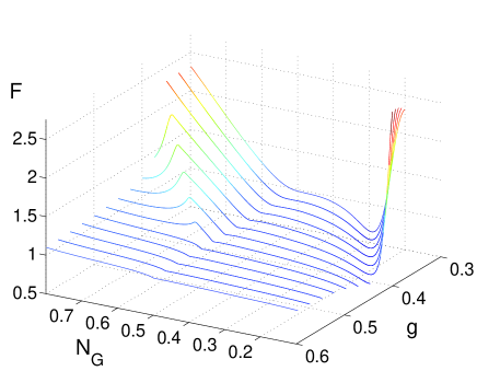
(a)

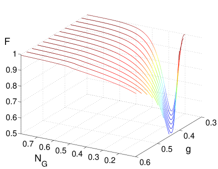
(b)

Figure 6: (color online) Fano factor $F\equiv S(0)/2eI$ as a function of the gate charge $N_{G}$ and LL interaction parameter $g$ for $R=100$ (highly asymmetric junctions) at $eV=2\varepsilon_{p}$ ($T=0$), (a) with no plasmon relaxation ($\gamma_{p}=0$) and (b) with fast plasmon relaxation ($\gamma_{p}=10^{4}$).

V.3 Numerical results

The limiting cases of no plasmon relaxation ($\gamma_{p}=0$) and a fast plasmon relaxation ($\gamma_{p}=10^{4}$) are summarized in Fig. 6(a) and (b), respectively. In the figure the Fano factor is plotted as a function of gate voltage and interaction parameter $g$ in the strong interaction regime $0.6\leq g\leq 0.3$ at $eV=2\varepsilon_{p}$ for $R=100$ (strongly asymmetric junctions).

As shown in Fig. 6(a), the Fano factor is enhanced above the Poisson limit ($F=1$) for a range of gate charges away from $N_{G}=1/2$, especially in the strong interaction regime, as expected from the three-state model. The shot noise enhancement is lost in the presence of a fast plasmon relaxation process, in agreement with analytic arguments, as seen in Fig. 6(b) when $F$ is bounded by $1/2\leq F\leq 1$. Hence, slowly relaxing plasmon excitations enhance shot noise, and this enhancement is most pronounced in the strongly interacting regime.

In the limit of fast plasmon relaxation $F$ exhibits a minimum value $F=1/2$ at positions consistent with predictions of the three-state model: the voltage polarity and ratio of tunneling matrix elements at the two junctions is such that total tunneling-in and tunneling-out rates are roughly equal for small values of $N_{G}$. If plasmon relaxation is slow, $F$ still has minima at approximately same values of $N_{G}$ but the minimal value of the Fano factor is considerably larger due to the presence of several transport channels.

V.4 Interplay between charge fluctuations and plasmon excitations near $eV=2E_{C}$

So far, we have investigated the role of non-equilibrium plasmons as the cause of the shot noise enhancement and focused on a voltage range when only two charge states are significantly involved in transport. The question naturally follows what is the consequence of the charge fluctuations. Do they enhance shot noise, too?

To answer this question, we first consider a toy model in which the plasmon excitations are absent during the single-charge transport. In the three-N-state regime where the relevant states are $\left|\textstyle N\right\rangle=\left|\textstyle-1\right\rangle,\left|\textstyle 0\right\rangle$ and $\left|\textstyle 1\right\rangle$ with no plasmon excitations at all. At zero temperature, the rate matrix in this regime is given by

$$\widehat{\mathbf{\textstyle\Gamma}}=\left[\begin{array}[]{ccc}\Gamma_{-1}^{+}&-\Gamma_{0}^{-}&0\\ -\Gamma_{-1}^{+}&\Gamma_{0}^{-}+\Gamma_{0}^{+}&-\Gamma_{1}^{-}\\ 0&-\Gamma_{0}^{+}&\Gamma_{1}^{-}\end{array}\right]~{},$$ (48)

where the matrix elements are $\Gamma_{i}^{+}=\Gamma_{L}(i+1,\{0\}\leftarrow i,\{0\}),\Gamma_{i}^{-}=\Gamma_{R}(i-1,\{0\}\leftarrow i,\{0\}),~{}i=-1,0,1$. Repeating the procedure in subsection V.2, we arrive at a Fano factor that has a similar form as Eq. (42),

$$F_{3N}=1-2[(1-P_{-1})P_{-1}+(1-P_{1})P_{1}]\\ +2P_{-1}P_{1}\left(\frac{\Gamma_{-1}^{+}}{\Gamma_{1}^{-}}+\frac{\Gamma_{1}^{-}}{\Gamma_{-1}^{+}}\right),$$ (49)

with the steady-state probability vector

$$\left|\textstyle P(\infty)\right\rangle=\left[\begin{array}[]{c}P_{-1}\\ P_{0}\\ P_{1}\end{array}\right]=\frac{1}{Z}\left[\begin{array}[]{c}\Gamma_{0}^{-}\Gamma_{1}^{-}\\ \Gamma_{-1}^{+}\Gamma_{1}^{-}\\ \Gamma_{-1}^{+}\Gamma_{0}^{+}\end{array}\right]$$ (50)

where $Z=\Gamma_{0}^{-}\Gamma_{1}^{-}+\Gamma_{-1}^{+}\Gamma_{1}^{-}+\Gamma_{-1}^{+}\Gamma_{0}^{+}$.

Despite the formal similarity of Eq. (49) with Eq. (42), its implication is quite different. In terms of the transition rates, $F_{3N}$ reads

$$F_{3N}=1-\frac{2}{Z^{2}}\Big{[}\Gamma_{1}^{-}\Gamma_{0}^{-}(\Gamma_{-1}^{+}\Gamma_{0}^{+}+(\Gamma_{-1}^{+}-\Gamma_{0}^{+})\Gamma_{1}^{-})\\ +\Gamma_{-1}^{+}\Gamma_{0}^{+}(\Gamma_{0}^{-}\Gamma_{1}^{-}+(\Gamma_{1}^{-}-\Gamma_{0}^{-})\Gamma_{1}^{-})\Big{]}.$$ (51)

Since $\Gamma_{-1}^{+}>\Gamma_{0}^{+}$ and $\Gamma_{1}^{-}>\Gamma_{0}^{-}$ in the three-N-state regime, the Fano factor $F_{3N}$ is sub-Poissonian, i.e., $F_{3N}<1$, consistent with the conventional equilibrium descriptions Hershfield et al. (1993); Braggio et al. (2003).

We conclude that while plasmon excitations may enhance the shot noise over the Poisson limit, charge fluctuations, in contrast, do not alter the sub-Poissonian nature of the Fano factor in the low energy regime. This qualitative difference is due to the fact that certain transition rates between different charge states vanish identically (in the absence of co-tunneling): it is impossible for the system to move directly from a state with $N=-1$ to $N=1$ or vice versa.

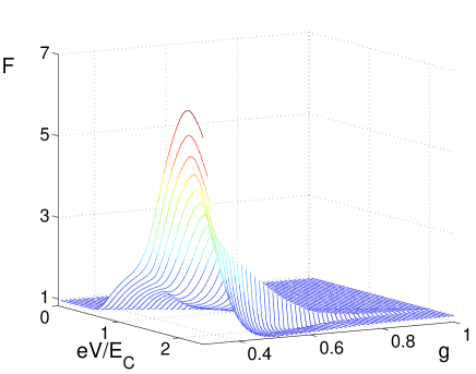
(a)

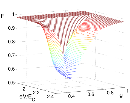
(b)

Figure 7: (color online) Fano factor $F\equiv S(0)/2eI$ as a function of the bias $eV$ and LL interaction parameter $g$ for $R=100$ (highly asymmetric junctions) at $N_{G}=1/2$ ($T=0$), (a) with no plasmon relaxation ($\gamma_{p}=0$) and (b) with fast plasmon relaxation ($\gamma_{p}=10^{4}$).

Therefore, we expect that for bias voltages near $eV=2E_{C}>2\varepsilon_{p}$, when both plasmon excitations and charge fluctuations are relevant, the Fano factor will exhibit complicated non-monotonic behavior. Exact solution is not tractable in this regime since it involves too many states. Instead, we calculate the shot noise numerically, with results depicted in Fig. 7, where the zero temperature Fano factor is shown as a function of the bias $eV$ and LL interaction parameter $g$ for $R=100$ at $N_{G}=1/2$, (a) with no plasmon relaxation ($\gamma_{p}=0$) and (b) with fast plasmon relaxation ($\gamma_{p}=10^{4}$).

In the bias regime up to the charging energy $eV\leq 2E_{C}$, the Fano factor increases monotonically due to non-equilibrium plasmons. On the other hand, the charge fluctuations contribute at $eV\geq 2E_{C}$ which tends to suppress the Fano factor. As a consequence of this competition, the Fano factor reaches its peak at $eV=2E_{C}$ and is followed by a steep decrease as shown in Fig. 7(a). Note the significant enhancement of the Fano factor in the strong interaction regime, which is due in part to the power law dependence of the transition rates with exponent $\alpha=(1/g-1)$ as discussed earlier, and in part to more plasmon states being involved for smaller $g$ since $E_{C}=\varepsilon_{p}/g$. The latter reason also accounts for the fact that the Fano factor begins to rise at a lower apparent bias for smaller $g$: the bias voltage is normalized by $E_{C}$ so that plasmon excitation is possible for lower values of $eV/E_{C}$ for stronger interactions.

In the case of fast plasmon relaxation, the rich structure of the Fano factor due to non-equilibrium plasmons is absent as shown in Fig. 7(b), in agreement with the discussions in previous subsections. The only remaining structure is a sharp dip around $eV=2E_{C}$ that can be attributed to the charge fluctuations at $eV\geq 2E_{C}$. Not only is the minimum value of the Fano factor a function of the interaction strength but also the bias voltage at which it occurs depends on $g$. The minimum Fano factor occurs at higher bias voltage, and the dip tends to be deeper with increasing interaction strength. Note for $g\lesssim 0.5$, the Fano factor did not reach its minimum still at largest voltages plotted ($eV/(2E_{C})=1.2$).

The Fano factor at very low voltages $eV<2\varepsilon_{p}$ for $N_{G}=1/2$ is $F^{(0)}=(1+R^{2})/(1+R)^{2}$ (see Eq. (35)), regardless of the plasmon relaxation mechanism. As shown in Fig. 7(b), the Fano factor is bounded above by this value in the case of fast plasmon relaxation. Notice that in the case of no plasmon relaxation (7(a)), the dips in the Fano factor at $eV>2E_{C}$ reach below $F^{(0)}$. See Fig. 1(a) in Ref. Kim et al., for more detail.

Since both the minimum value of $F$ and the voltage at which it occurs are determined by a competition between charge fluctuations and plasmonic excitations, they cannot be accurately predicted by any of the simple analytic models discussed above.

V.5 Finite frequency noise

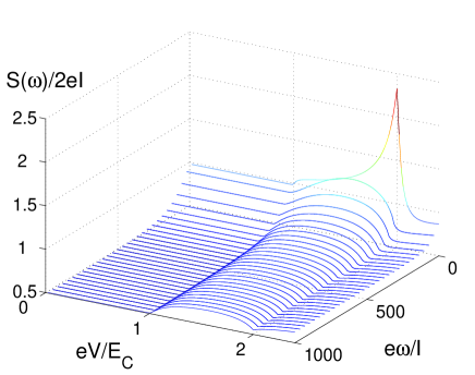
(a)

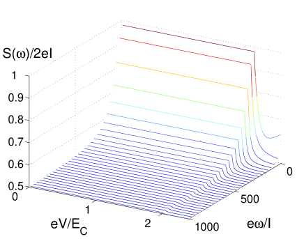
(b)

Figure 8: (color online) Finite frequency shot noise $S(\omega)/2eI$ as a function of the bias $eV/E_{C}$ and frequency $e\omega/I$ for $R=100$ and $g=0.5$, at $N_{G}=1/2$ ($T=0$), (a) with no plasmon relaxation ($\gamma_{p}=0$) and (b) with fast plasmon relaxation ($\gamma_{p}=10^{4}$).

In the high frequency limit, $\omega\rightarrow\infty$, the correlation effects are lost in the noise power (30) except the $\delta(\tau)$-term in Eq. (31) that reflects the Pauli exclusion Korotkov et al. (1992), and the asymptotic value of the noise spectrum reduces to

$$S(\infty)=2e\left(\frac{C_{R}^{2}A_{L}}{(C_{L}+C_{R})^{2}}+\frac{C_{L}^{2}A_{R}}{(C_{L}+C_{R})^{2}}\right)=\frac{e}{2}(A_{L}+A_{R}),$$ (52)

where

$$A_{\ell}=e\sum_{N,\{n\}}\langle N,\{n\}|\widehat{\mathbf{\textstyle\Gamma}}^{+}_{\ell}+\widehat{\mathbf{\textstyle\Gamma}}^{-}_{\ell}|P(\infty)\rangle$$ (53)

is the total tunneling rate across the junction $\ell$ without regard to direction.

The decay of the current-current correlations at finite frequencies is depicted in Fig. 8, where the shot noise power $S(\omega)/2eI$ is shown as a function of the bias and the frequency for a strong interaction ($g=0.5$) and the strongly asymmetric tunnel barriers ($R=100)$ (a) with no plasmon relaxation and (b) with fast plasmon relaxation ($\gamma_{p}=10^{4}$).

In the regime of the elastic process, in which the charge transport does not involve excitations (plasmons) in the dot, the backward tunneling against the bias is blocked at zero temperature. In this regime, the rate density is equal to the average current, $A_{L}=A_{R}=I$, and the high frequency noise power asymptotically converges to its minimum value $S(\infty)=eI$. This is clearly seen in the regime of the low bias $eV<2\varepsilon_{p}(=E_{C})$ in Fig. 8(a) and (b).

In the presence of fast plasmon relaxation, still no backward tunneling is possible and the shot noise reaches its minimum value $S(\infty)=eI$ at high frequency limit (see Fig. 8(b)). However, the non-equilibrium plasmons excited above the Fermi energies of the leads invoke non-vanishing backward tunneling and the high frequency shot noise remains above $eI$, as shown in the bias regime of $eV>2\varepsilon_{p}$ in Fig. 8(a).

Another identifiable feature in Fig. 8(a) is the rapid decrease of the shot noise power as a function of $\omega$ at those voltages when the Fano factor has a maximum. The maxima occur at voltages when additional states become significantly populated, and the characteristic low frequency reflects the slow transition rates to states near their energy thresholds.

VI Full counting statistics

Since shot noise that is a current-current correlation is more informative than the average current, we expect more information with higher-order currents or charge correlations. The method of counting statistics, which was introduced to mesoscopic physics by Levitov and Lesovik (1993) followed by Muzykantskii and Khmelnitskii (1994) and Lee et al. (1995), shows that all orders of charge correlation functions can be obtained as a function related to the probability distribution of transported electrons for a given time interval. This powerful approach is known as full counting statistics (FCS). The first experimental study of the third cumulant of the voltage fluctuations in a tunnel junction was carried out by Reulet et al. (2003). The experiment indicates that the high cumulants are more sensitive to the coupling of the system to the electromagnetic environment. See also Levitov and Lesovik (2004) and Beenakker et al. (2003) for the theoretical discussions on the third cumulant in a tunnel-barrier.

de Jong (1996) showed that the low-energy physics of the FCS calculations both with quantum mechanical and semiclassical approaches are identical in the DB structures, as in the explicit shot noise calculations, except for a short initial time scale.

We will now carry out an FCS analysis of transport through a double barrier quantum wire system. The analysis will provide a more complete characterization of the transport properties of the system than either average current or shot noise, and shed further light on the role of non-equilibrium vs. equilibrium plasmon distribution in this structure.

Let $P(M,\tau)$ be the probability that $M$ electrons have tunneled across the right junction to the right lead during the time $\tau$. We note that

$$P(M,\tau)=\lim_{t\to\infty}\sum_{N,\left\{\textstyle n\right\}}\sum_{M_{0},N_{0},\left\{\textstyle n_{0}\right\}}\\ P(M_{0}+M,N,\left\{\textstyle n\right\},t+\tau;M_{0},N_{0},\left\{\textstyle n_{0}\right\},t),$$

where $P(M_{0}+M,N,\left\{\textstyle n\right\},t+\tau;M_{0},N_{0},\left\{\textstyle n_{0}\right\},t)$ is called joint probability since it is the probability that, up to time $t$, $M_{0}$ electrons have passed across the right junction and $N_{0}$ electrons are confined in the QD with $\left\{\textstyle n_{0}\right\}$ plasmon excitations, and that $M_{0}+M$ electrons have passed R–junction with $(N,\{n\})$ excitations in the QD up to time $t+\tau$. The master equation for the joint probability can easily be constructed from Eq. (23) by noting that $M\to M\pm 1$ as $N\to N\mp 1$ via only R–junction hopping.

To obtain $P(M,\tau)$, it is convenient to define the characteristic function conjugate to the joint probability as

$$g(\theta,N,\left\{\textstyle n\right\},\tau)=\lim_{t\to\infty}\sum_{M}e^{-i\theta M}\sum_{M_{0},N_{0},\left\{\textstyle n_{0}\right\}}\\ P(M_{0}+M,N,\left\{\textstyle n\right\},t+\tau;M_{0},N_{0},\left\{\textstyle n_{0}\right\},t).$$

The characteristic function satisfies the master equation

$$\frac{\partial}{\partial\tau}\left|\textstyle g(\theta,\tau)\right\rangle=-\widehat{\mathbf{\textstyle\Gamma}}(\theta)\left|\textstyle g(\theta,\tau)\right\rangle$$ (54)

with the initial condition $\left|\textstyle g(\theta,\tau=0)\right\rangle=\left|\textstyle P(\infty)\right\rangle$. The $\theta$-dependent $\widehat{\mathbf{\textstyle\Gamma}}$ in Eq. (54) is related to the previously defined transition rate matrices through

$$\widehat{\mathbf{\textstyle\Gamma}}(\theta)=\widehat{\Gamma}_{p}+\left(\widehat{\mathbf{\textstyle\Gamma}}_{L}^{0}-\widehat{\mathbf{\textstyle\Gamma}}_{L}^{+}-\widehat{\mathbf{\textstyle\Gamma}}_{L}^{-}\right)+\left(\widehat{\mathbf{\textstyle\Gamma}}_{R}^{0}-\widehat{\mathbf{\textstyle\Gamma}}_{R}^{+}e^{+i\theta}-\widehat{\mathbf{\textstyle\Gamma}}_{R}^{-}e^{-i\theta}\right)\,.$$ (55)

The characteristic function $G(\theta,\tau)$ conjugate to $P(M,\tau)$ is now given by $G(\theta,\tau)=\sum_{N,\left\{\textstyle n\right\}}\left\langle\textstyle N,\left\{\textstyle n\right\}|g(\theta,\tau)\right\rangle$, or

$$G(\theta,\tau)=\sum_{N,\left\{\textstyle n\right\}}\left\langle\textstyle N,\left\{\textstyle n\right\}\right|\exp\left[-\widehat{\mathbf{\textstyle\Gamma}}(\theta)\tau\right]\left|\textstyle P(\infty)\right\rangle\,.$$ (56)

Finally, the probability $P(M,\tau)$ is obtained by

$$P(M,\tau)=\int_{0}^{2\pi}\frac{d\theta}{2\pi}\;e^{+i\theta M}G(\theta,\tau)=\oint\frac{dz}{2\pi i}\frac{G(z,\tau)}{z^{2M+1}}$$ (57)

with $z=e^{-i\theta/2}$, where the contour runs counterclockwise along the unit circle and we have used the symmetry property $G(z,\tau)=G(-z,\tau)$ for the second equality.

Taylor expansion of the logarithm of the characteristic function in $i\theta$ defines the cumulants or irreducible correlators $\kappa_{k}(\tau)$:

$$\ln G(\theta,\tau)=\sum_{k=1}^{\infty}\frac{(i\theta)^{k}}{k!}\kappa_{k}(\tau)\>.$$ (58)

The cumulants have a direct polynomial relation with the moments $\overline{n^{k}(\tau)}\equiv\sum_{n}n^{k}P(n,\tau)$. The first two cumulants are the mean and the variance, and the third cumulant characterizes the asymmetry (or skewness) of the $P(M,\tau)$ distribution and is given by

$$\kappa_{3}(\tau)=\overline{\delta n(\tau)^{3}}=\overline{(n(\tau)-\overline{n(\tau)})^{3}}.$$ (59)

In this section, we investigate FCS mainly in the context of the probability $P(M,\tau)$ that M electrons have passed through the right junction during the time $\tau$. Since the average current and the shot noise are proportional to the average number of the tunneling electrons $\left\langle\textstyle M\right\rangle$ and the width of the distribution of $P(M,\tau)$, respectively, we focus on the new aspects that are not covered by the study of the average current or shot noise.

In order to get FCS in general cases we integrate the master equation (54) numerically (see subsection VI.3). In the low-bias regime, however, some analytic argument can be made. We will show through the following subsections that for symmetric junctions in the low-bias regime ($2\varepsilon_{p}<eV<2E_{C}$), and irrespective of the junction symmetry in the very low bias regime ($eV<2\varepsilon_{p}$), $P(M,\tau)$ is given by the residue at $z=0$ alone,

$$P(M,\tau)=\frac{1}{(2M)!}\left.\frac{d^{2M}}{dz^{2M}}\right|_{z=0}G(z,\tau)\,.$$ (60)

Through this section we assume that the gate charge is $N_{G}=1/2$, unless stated explicitly not so.

We will now follow the outline of the previous section and start by considering two analytically tractable cases before proceeding with the full numerical results.

VI.1 Two-state process; $eV\approx\varepsilon_{p}$

For the very low bias $eV<2\varepsilon_{p}$ at zero temperature, no plasmons are excited and electrons are carried by transitions between two states $(N,n)=(0,0)\leftrightarrow(1,0)$. In this simplest case, the rate matrix $\widehat{\mathbf{\textstyle\Gamma}}(\theta)$ in Eq. (54) is determined by only two participating transition rates $\gamma^{+}=\Gamma_{L}(1,0\leftarrow 0,0)$ and $\gamma^{-}=\Gamma_{R}(0,0\leftarrow 1,0)$,

$$\widehat{\mathbf{\textstyle\Gamma}}(\theta)=\left[\begin{array}[]{cc}\Gamma_{0}+\delta&-(\Gamma_{0}-\delta)e^{-i\theta}\\ -(\Gamma_{0}+\delta)&\Gamma_{0}-\delta\end{array}\right]$$ (61)

with $\Gamma_{0}\equiv(\gamma^{+}+\gamma^{-})/2,~{}\delta\equiv(\gamma^{+}-\gamma^{-})/2$.

Substituting the steady-state probability Eq. (34) and the transition rate matrix (61) to Eq. (56), one finds

$$G_{2}(z,\tau)=\frac{e^{-\Gamma_{0}\tau}}{4}\frac{1}{f_{2}(z)}\bigg{[}(1+f_{2}(z))^{2}e^{+\Gamma_{0}\tau f_{2}(z)}\\ -(1-f_{2}(z))^{2}e^{-\Gamma_{0}\tau f_{2}(z)}\bigg{]},$$ (62)

where $f_{2}(z)=(\Gamma_{\delta}/\Gamma_{0})\sqrt{z^{2}+\Delta^{2}}$, with $\Gamma_{\delta}=\sqrt{\Gamma_{0}^{2}-\delta^{2}}=\sqrt{\gamma^{+}\gamma^{-}}$ and $\Delta^{2}=\delta^{2}/\Gamma_{\delta}^{2}$.

Now, it is straightforward to calculate the cumulants. In the long time limit $\tau\gg(\gamma^{\pm})^{-1}$, for instance, in terms of the average current $I_{2}=e\gamma^{+}\gamma^{-}/(\gamma^{+}+\gamma^{-})$ and the Fano factor $F_{2}$ in (35), the three lowest cumulants are given by

$$\kappa_{1}(\tau)=I_{2}\tau,\quad\kappa_{2}(\tau)=eI_{2}F_{2}\tau,$$

$$\kappa_{3}(\tau)=e^{2}I_{2}(3(F_{2}-1/2)^{2}+1/4)\tau,$$ (63)

where the electron charge ($-e$) is revived. These are in agreement with the phase-coherent quantum-mechanical results de Jong (1996). It is convenient to discuss the asymmetry (skewness) by the ratio $A\equiv\kappa_{3}/e^{2}\kappa_{1}$ ($\tau\to\infty$), noticing the Fano factor $F=\lim_{\tau\to\infty}\kappa_{2}(\tau)/e\kappa_{1}(\tau)$. The factor $A_{2}=3(F_{2}-1/2)^{2}+1/4$ is positive definite (positive skewness) and bounded by $1/4\leq A_{2}\leq 1$. It is interesting to notice that $A_{2}$ is a monotonic function of $F_{2}$ and has its minimum $A_{2}=1/4$ for the minimum $F_{2}=1/2$ and maximum $A_{2}=1$ for the maximum $F_{2}=1$. Notice $A=1$ for a Poissonian and $A=0$ for a Gaussian distribution. Therefore, the dependence of $A_{2}$ on the gate charge $N_{G}$ is similar to that of the Fano factor $F_{2}$ (see Fig. 4) with dips at $N_{G}^{\mathrm{dip}}$ in Eq. (38). Together with Eq. (37), it implies that the effective shot noise and the asymmetry of the probability distribution per unit charge transfer have their respective minimum values at the gate charge $N_{G}^{\mathrm{dip}}$ which depends on the tunnel-junction asymmetry and the interaction strength of the leads.

Figure 9: Contour of Eq. (57). The arguments of $f_{2}(z)=(\Gamma_{\delta}/\Gamma_{0})\sqrt{z^{2}+\Delta^{2}}~{}$ are $\pi/2,-\pi/2,\pi/2,-\pi/2$ along the branch cuts $C_{1},C_{2},C_{3}$, and $C_{4}$, respectively.

The integral in Eq. (57) is along the contour depicted in Fig. 9. Notice that the contributions from the part along the branch cuts are zero and we are left with the multiple poles at $z=0$. By residue theorem, the two-state probability $P_{2}(M,\tau)$ is given by Eq. (60).

The exact expression of $P_{2}(M,\tau)$ is cumbersome. For symmetric tunneling barriers with $N_{G}=1/2$ ($\delta=0,~{}\gamma^{+}=\gamma^{-}=\Gamma_{0}$), however, Eq. (62) reduces to

$$G_{2}^{(s)}(z,\tau)=\frac{e^{-\Gamma_{0}\tau}}{4z}\Big{(}(1+z)^{2}e^{+\Gamma_{0}\tau z}-(1-z)^{2}e^{-\Gamma_{0}\tau z}\Big{)}.$$ (64)

Accordingly, $P^{(s)}_{2}(M,\tau)$ is concisely given by

$$P^{(s)}_{2}(M,\tau)=e^{-\Gamma_{0}\tau}\bigg{[}\frac{1}{2}\frac{(\Gamma_{0}\tau)^{2M-1}}{(2M-1)!}+\frac{(\Gamma_{0}\tau)^{2M}}{(2M)!}\\ +\frac{1}{2}\frac{(\Gamma_{0}\tau)^{2M+1}}{(2M+1)!}\bigg{]},\mbox{ for }~{}M\geq 1,$$ (65)

with $P^{(s)}_{2}(0,\tau)=e^{-\Gamma_{0}\tau}(1+\Gamma_{0}\tau/2)$, in agreement with Eq. (24) of Ref. de Jong, 1996. While this distribution resembles a sum of three Poisson distributions, it is not exactly Poissonian.

For a highly asymmetric junctions $R\gg 1$ $(\gamma^{+}\gg\gamma^{-})$, the first term in Eq. (62) dominates the dynamics of $G_{2}(z,\tau)$ and its derivatives, and the characteristic function is approximated by

$$G_{2}^{(a)}(z,\tau)\approx\exp\left(-\tau\Gamma_{0}+\tau\sqrt{(\gamma^{+}\gamma^{-})z^{2}+\delta^{2}}\right).$$ (66)

Now, the solution of $P^{(a)}_{2}(M,\tau)$ is calculated by this equation and Eq. (60). The leading order approximation in $\gamma^{-}/\gamma^{+}$ leads to the Poisson distribution,

$$P^{(a)}_{2}(M,\tau)\approx\frac{(\gamma^{-}\tau)^{M}}{M!}e^{-\gamma^{-}\tau}.$$ (67)

For a single tunneling-barrier, the charges are transported by the Poisson process ($F=1$) Blanter and Büttiker (2000). Therefore, we recover the Poisson distribution in the limit of strongly asymmetric junctions and in the regime of the two-state process, in which electrons see effectively single tunnel-barrier.

For the intermediate barrier asymmetry, therefore, the probability $P_{2}(M,\tau)$ of a two-state process is given by a distribution between Eq. (65) (for symmetric–junctions) and the Poissonian (67) (for the most asymmetric–junctions).

VI.2 Four-state process; $2\varepsilon_{p}\lesssim eV\lesssim 2E_{C}$

Since we focus the FCS analysis on the case $N_{G}=1/2$, the next simplest case to study is a four-state-model rather than the three-state-model discussed in the connection of the shot noise in the previous section.

In the bias regime where the transport is governed by Coulomb blockade ($eV<2E_{C}$) and yet the plasmons play an important role ($eV\geq 2\varepsilon_{p}$), it is a fairly good approximation to include only the four states with $N=0,1$ and $n_{1}=0,1$ ($n_{m}=0$ for $m\geq 2$). For general asymmetric cases, the rate matrix $\widehat{\mathbf{\textstyle\Gamma}}(\theta)$ in Eq. (54) is determined by ten participating transition rates (four rates from each junction, and two relaxation rates). The resulting eigenvalues of $\left|\textstyle g(\theta,\tau)\right\rangle$ are the solutions of a quartic equation, which is in general very laborious to solve analytically.

For symmetric junctions ($R=1$) with no plasmon relaxation, however, the rate matrix is simplified to

$$\widehat{\mathbf{\textstyle\Gamma}}(\theta)=\left[\begin{array}[]{cccc}\gamma_{00}+\gamma_{10}&0&-\gamma_{00}z^{2}&-\gamma_{01}z^{2}\\ 0&\gamma_{01}+\gamma_{11}&-\gamma_{10}z^{2}&-\gamma_{11}z^{2}\\ -\gamma_{00}&-\gamma_{01}&\gamma_{00}+\gamma_{10}&0\\ -\gamma_{10}&-\gamma_{11}&0&\gamma_{01}+\gamma_{11}\end{array}\right]$$ (68)

with the matrix elements $\gamma_{ij}\equiv\Gamma_{L}(1,i\leftarrow 0,j)=\Gamma_{R}(0,i\leftarrow 1,j)$. The steady-state probability is then given by

$$\left|\textstyle P_{4}^{(s)}(\infty)\right\rangle=\left|\textstyle g(z,\tau=0)\right\rangle=\frac{1}{2(\gamma_{01}+\gamma_{10})}\left[\begin{array}[]{l}\gamma_{01}\\ \gamma_{10}\\ \gamma_{01}\\ \gamma_{10}\end{array}\right]$$ (69)

Solving Eq. (56) with this probability and the rate matrix (68) is laborious but straightforward and one finds

$$G(z,\tau)=e^{-(\gamma_{00}+\gamma_{10}+\gamma_{01}+\gamma_{11})\tau/2}\\ \times\bigg{[}\Big{\{}G_{I}(z,\tau)\frac{(1+z)^{2}}{8z}\Big{\}}+\Big{\{}z\to-z\Big{\}}\bigg{]},$$ (70)

with

$$G_{I}(z,\tau)=\bigg{\{}e^{(\gamma_{00}z+\gamma_{11}z+f_{4}(z))\tau/2}\left(1+\frac{A(z)}{f_{4}(z)}\right)\\ \times\left(1-\frac{A(z)-f_{4}(z)}{2(\gamma_{01}+\gamma_{10})z}\right)\bigg{\}}+\bigg{\{}f_{4}(z)\to-f_{4}(z)\bigg{\}},$$ (71)

where $A(z)$ and $f_{4}(z)$ are given by

$$A(z) = \gamma_{00}+\gamma_{10}-\gamma_{01}-\gamma_{11}-(\gamma_{00}-\gamma_{11}-2\gamma_{01})z$$

$$f_{4}(z) = \sqrt{(\gamma_{00}-\gamma_{11})^{2}-4\gamma_{10}\gamma_{01}}\sqrt{(z-a)^{2}+b^{2}}$$ (72)

with dimensionless parameters $a,b$ given by

$$a = \frac{(\gamma_{00}-\gamma_{11})(\gamma_{00}+\gamma_{10}-\gamma_{01}-\gamma_{11})}{(\gamma_{00}-\gamma_{11})^{2}-4\gamma_{10}\gamma_{01}},$$

$$b = \frac{\sqrt{4\gamma_{10}\gamma_{01}}(\gamma_{00}+\gamma_{10}-\gamma_{01}-\gamma_{11}))}{(\gamma_{00}-\gamma_{11})^{2}-4\gamma_{10}\gamma_{01}}.$$

Integral of $G_{I}(z,\tau)$ along the contour $|z|=1$ contains two branch points at $z_{c}=a\pm ib$, however, the integral along the branch cuts cancel out due to the symmetry under $[f_{4}(z)\to-f_{4}(z)]$. Therefore, the contribution from the branch cuts due to $G_{I}(z,\tau)$ and $G_{I}(-z,\tau)$ is zero to the probability $P_{4}^{(s)}(M,\tau)$, and it is given by the residues only at $z=0$, i.e. by Eq. (60). The explicit expression of $P_{4}^{(s)}(M,\tau)$ is cumbersome.

The probability distribution $P_{2}(M,\tau)$ for the two-state process deviates from Eq. (65) as a function of the asymmetry parameter $R$ and reaches Poissonian in the case of strongly asymmetric–junctions. In a similar manner, $P_{4}^{(s)}(M,\tau)$ deviates from $P_{2}^{(s)}(M,\tau)$ as a function of ratio of the transition rates $\gamma_{ij}$.

VI.3 Numerical results

It is worth mentioning that for strongly asymmetric junctions $P(M,\tau)$ is Poissonian in the very low bias regime ($eV<2\varepsilon_{p}$), as seen in Eq. (67). It exhibits a crossover at $eV=2\varepsilon_{p}$: $P(M,\tau)$ deviates from Poisson distribution for $2\varepsilon_{p}<eV<2E_{C}$ while it is Poissonian for $eV<2\varepsilon_{p}$ (at $T=0$), as shown by the shot noise calculation.

VI.3.1 Voltage dependence

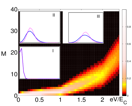
(a)

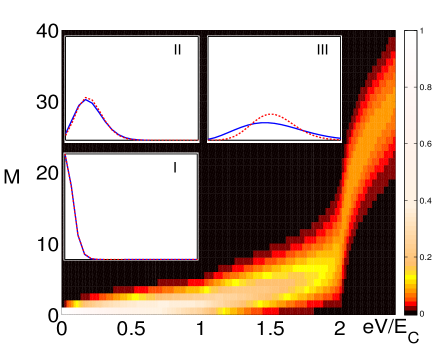
(b)

Figure 10: (color online) Probability $P(M,\tau)$ with no plasmon relaxation ($\gamma_{p}=0$) during the time $\tau=10/I_{c}$, where $I_{c}$ is the particle current at $eV=2E_{C}$ with no plasmon relaxation ($\gamma_{p}=0$); (a) for symmetric junctions ($R=1$) and (b) for a highly asymmetric junctions ($R=100$). Here $g=0.5$, $N_{G}=1/2$, and $T=0$. Inset shows cross-sectional image of $P(M,\tau)$ (blue solid line) as a function of $M$ and the reference distribution function (a) Eq. (65) (magenta dashed line) and (b) the Poisson distribution Eq. (67) (red dashed), at (I) $eV=0.5E_{C}$, (II) $eV=1.5E_{C}$, and (III) $eV=2E_{C}$.

The analytic results presented above are useful in interpreting the numerical results in Fig. 10, where probability $P(M,\tau)$ for (a) symmetric junctions ($R=1$) and (b) $R=100$, in the case of LL parameter $g=0.5$ with no plasmon relaxation ($\gamma_{p}=0$), is shown as a function of $eV$ and $M$ that is the number of transported electrons to the right lead during $\tau$ such that during this time $\left\langle\textstyle M\right\rangle=I_{c}\tau=10$ electrons have passed to the right lead at $eV=2E_{C}$.

The peak position of the distribution of $P(M,\tau)$ is roughly linearly proportional to the average particle flow $\left\langle\textstyle M\right\rangle$, and the width is proportional to the shot noise but in a nonlinear manner. In a rough estimate, therefore, the ratio of the peak width to the peak position is proportional to the Fano factor. Two features are shown in the figure. First, the average particle flow (the peak position) runs with different slope when the bias voltage crosses new energy levels, i.e. at $eV=2\varepsilon_{p}$ and $eV=2E_{C}$, that is consistent with the $I-V$ study (compare Fig. 10(b) with Fig. 3). Notice $E_{C}=\varepsilon_{p}/g=2\varepsilon_{p}$ for $g=0.5$. Second, the width of the distribution increases with increasing voltage, with different characteristics categorized by $eV=2\varepsilon_{p}$ and $eV=2E_{C}$. Especially in the bias regime $eV>2E_{C}$ in which the charge fluctuations participate to the charge transport, for the highly asymmetric case, the peak runs very fast while its width does not show noticeable increase. It causes the dramatic peak structure in the Fano factor around $eV=2E_{C}$ as discussed in section V.

The deviation of the distribution of probability $P(M,\tau)$ due to the non-equilibrium plasmons from its low voltage (equilibrium) counterpart is shown in the insets. Notice in the low bias regime $eV<2\varepsilon_{p}$, it follows Eq. (65) for the symmetric case (10(a), inset I), and the Poissonian distribution (67) for the highly asymmetric case (10(b), inset I). The deviation is already noticeable at $eV=3\varepsilon_{p}=1.5E_{C}$ for $R=1$ (inset II in 10(a)), while it deviates strongly around $eV=2E_{C}$ for $R=100$ (inset III in 10(a)).

VI.3.2 Interaction strength dependence

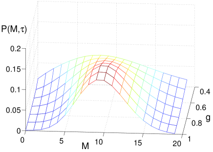
(a)

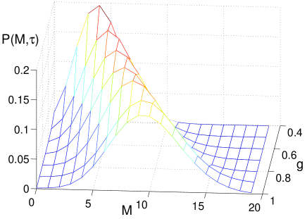
(b)

Figure 11: (color online) The probability $P(M,\tau)$ that M electrons have passed through the right junction during the time $\tau=10/I_{0}$, where $I_{0}$ is the particle current with no plasmon relaxation ($\gamma_{p}=0$); (a) with no plasmon relaxation ($\gamma_{p}=0$) and (b) with fast plasmon relaxation ($\gamma_{p}=10^{4}$). Here $eV=2E_{C},R=100,N_{G}=1/2$ and $T=0$.

We have concluded in section V that shot noise shows most dramatic behavior around $eV=2E_{C}$ due to interplay between the non-equilibrium plasmons and the charge fluctuations. To see its consequence in FCS, we plot in Fig. 11 the probability $P(M,\tau)$ as a function of the particle number $M$ and the interaction parameter $g$ for $\tau=10e/I(eV=2E_{C},\gamma_{p}=0)$ (a) with no plasmon relaxation and (b) with fast plasmon relaxation.

The main message of Fig. 11(a) is that the shot noise enhancement, i.e. the broadening of the distribution curve, is significant in the strong interaction regime with gradual increase with decreasing $g$. Fast plasmon relaxation consequently suppresses the average current dramatically as shown in Fig. 11(b) implying the Fano factor enhancement is lost. Effectively, the probability distribution of $P(M,\tau)$ for different interaction parameters maps on each other almost identically if the time duration is chosen such that $\left\langle\textstyle M\right\rangle$ equals for all $g$.

VII Conclusions

We have studied different transport properties of a Luttinger-liquid single-electron transistor including average current, shot noise, and full counting statistics, within the conventional sequential tunneling approach.

At finite bias voltages, the occupation probabilities of the many-body states on the central segment is found to follow a highly non-equilibrium distribution. The energy is transferred between the leads and the quantum dot by the tunneling electrons, and the electronic identity is dispersed into the plasmonic collective excitations after the tunneling event. In the case of nearly symmetric barriers, the distribution of the occupation probabilities of the non-equilibrium plasmons shows impressive contrast depending on the interaction strength: In the weakly interacting regime, it is a complicated function of the many-body occupation configuration, while in the strongly interacting regime, the occupation probabilities are determined almost entirely by the state energies and the bias voltage, and follow a universal distribution resembling Gibbs (equilibrium) distribution. This feature in the strong interaction regime fades out with the increasing asymmetry of the tunnel–barriers.

We have studied the consequences of these non-equilibrium plasmons on the average current, shot noise, and counting statistics. Most importantly, we find that the average current is increased, shot noise is enhanced beyond the Poisson limit, and full counting statistics deviates strongly from the Poisson distribution. These non-equilibrium effects are pronounced especially in the strong interaction regime, i.e. $g\lesssim 0.5$. The overall transport properties are determined by a balance between phenomena associated with non-equilibrium plasmon distribution that tend to increase noise, and charge fluctuations that tend to decrease noise. The result of this competition is, for instance, a non-monotonic voltage dependence of the Fano factor.

At the lowest voltages when charge can be transported through the system, the plasmon excitations are suppressed, and the Fano factor is determined by charge fluctuations. Charge fluctuations are maximized when the tunneling-in and tunneling-out rates are equal, which for symmetric junctions occurs at gate charge $N_{G}=1/2$. At these gate charges the Fano factor acquires its lowest value which at low voltages is given by a half of the Poisson value, known as $1/2$ suppression, as only two states are involved in the transport, at somewhat larger voltages increases beyond the Poisson limit as plasmon excitations are allowed, and at even higher voltages exhibits a local minimum when additional charge states are important. If the non-equilibrium plasmon effects are suppressed e.g. by fast plasmon relaxation, only the charge fluctuation effects survive, and the Fano factor is reduced below its low-voltage value. The non-equilibrium plasmon effects are also suppressed in the non-interacting limit.

Appendix A The transition amplitudes in the quantum dot

In this appendix, we derive the transition amplitudes, Eqs. (15) and (16). As shown in Eq. (14), the zero-mode overlap of the QD transition amplitude is unity or zero. Therefore, we focus on the overlap of the plasmon states. It is enough to consider

$$|\langle\{n^{\prime}\}|\Psi^{\dagger}_{D}(X_{\ell})|\{n\}\rangle|^{2},~{}~{}X_{\ell}=X_{L},X_{R}$$

due to the symmetry between matrix elements of tunneling-in and tunneling-out transitions, as in Eq. (15),

$$|\langle\{n^{\prime}\}|\Psi^{\dagger}(X_{\ell})|\{n\}\rangle|^{2} = ~{}\sum_{r=\pm}\Big{[}|\langle\{n^{\prime}\}|\psi^{\dagger}_{r}(X_{\ell})|\{n\}\rangle|^{2}+\langle\{n^{\prime}\}|\psi^{\dagger}_{r}(X_{\ell})|\{n\}\rangle\langle\{n\}|\psi_{-r}(X_{\ell})|\{n^{\prime}\}\rangle\Big{]}$$ (73)

$$= 2|\langle\{n^{\prime}\}|\psi^{\dagger}_{r}(X_{\ell})|\{n\}\rangle|^{2},$$

where $r=+(-)$ denotes the right(left)–moving component, and the cross terms of oppositely moving components cancel out due to fermionic anti-commutation relations.

The transition amplitudes at $X_{L}$ is identical to that at $X_{R}$. For simplicity, we consider the case at $X_{L}=0$ only. The overlap elements of the many-body occupations $\left\langle\textstyle\{n\}\right|=\left\langle\textstyle n_{1},n_{2},\cdots,n_{m},\cdots\right|$ and $\left|\textstyle\{n^{\prime}\}\right\rangle=\left|\textstyle n_{1}^{\prime},n_{2}^{\prime},\cdots,n_{m}^{\prime},\cdots\right\rangle$ are

$$|\langle\{n\}|\psi^{\dagger}_{r}(x=0)|\{n^{\prime}\}\rangle|^{2}=\frac{1}{2\pi\Lambda}\prod_{m=1}^{\infty}|\langle n_{m}|\varphi_{m}|n_{m}^{\prime}\rangle|^{2},$$ (74)

where $\varphi_{m}=\exp\left[\lambda_{m}(b_{m}+b_{m}^{\dagger})\right]$ with $\lambda_{m}=-\frac{i}{\sqrt{gmM}}$ is the bosonized field operator at an edge of the wire with open boundary conditions (see for instance Ref. Mattsson et al., 1997). Here $g$ is the interaction parameter, $m$ is the mode index (and the integer momentum of it), and $M$ is the number of transport sectors; if $M>1$, the contributions of the different sectors must be multiplied. The operators $b_{m}$ and $b_{m}^{\dagger}$ denote plasmon annihilation and creation and $\Lambda$ is a high energy cut-off.

Using the Baker-Haussdorf formula

$$\varphi_{m}=\exp\left[\lambda_{m}(a_{m}+a_{m}^{\dagger})\right]=e^{-\frac{\lambda^{2}}{2}}e^{\lambda_{m}a_{m}}e^{\lambda_{m}a^{\dagger}_{m}},$$ (75)

and the harmonic oscillator states

$$|n\rangle=\frac{(a^{\dagger})^{n}}{\sqrt{n!}}|0\rangle,~{}~{}~{}\langle n|=\langle 0|\frac{a^{n}}{\sqrt{n!}},$$ (76)

one can show that, if $n\leq n^{\prime}$,

$$|\left\langle\textstyle n|\varphi|n^{\prime}\right\rangle|^{2}=e^{|\lambda|^{2}}\frac{|\lambda|^{2(n-n^{\prime})}}{n!n^{\prime}!}\left(\frac{n!}{(n-n^{\prime})!}\right)^{2}\\ \times\Phi(n+1,n-n^{\prime}+1;-|\lambda|^{2})^{2},$$ (77)

where $\Phi(x,x^{\prime};z)$ is a degenerate hypergeometric function defined by Gradshteyn and Ryzhik (1980)

$$\Phi(x,x^{\prime};z)=\left[\sum_{\ell=0}^{\infty}\frac{z^{\ell}}{\ell!}\frac{(x-1+\ell)!}{(x-1)!}\frac{(x^{\prime}-1)!}{(x^{\prime}-1+\ell)!}\right].$$ (78)

If $n^{\prime}\leq n$, the indices $n$ and $n^{\prime}$ are exchanged in Eq. (77). The function $\Phi(x,x^{\prime};z)$ is a solution of the equation

$$z\partial^{2}_{z}\Phi+(x^{\prime}-z)\partial_{z}\Phi-x\Phi=0.$$

By solving this differential equation with the proper normalization constant, one obtains

$$\Phi(n+1,n-n^{\prime}+1;-|\lambda|^{2})=\frac{n^{\prime}!(n-n^{\prime})!}{n!}e^{-|\lambda|^{2}}L_{n^{\prime}}^{n-n^{\prime}}(|\lambda|^{2}),$$

where $L_{a}^{b}(y)$ is the Laguerre polynomials Gradshteyn and Ryzhik (1980). In terms of the Laguerre polynomials, therefore, the transition amplitude (77) is written by

$$|\langle n_{m}|\varphi_{m}|n_{m}^{\prime}\rangle|^{2}=\frac{e^{-1/gmM}}{(gmM)^{|n_{m}^{\prime}-n_{m}|}}\frac{n_{m}^{(<)}!}{n_{m}^{(>)}!}\\ \times\left[L^{|n_{m}^{\prime}-n_{m}|}_{n_{m}^{(<)}}\left(\frac{1}{gmM}\right)\right]^{2}$$ (79)

where $n^{(<)}=\min(n^{\prime},n)$ and $n^{(>)}=\max(n^{\prime},n)$.

We introduce a high frequency cut-off $m_{c}\sim k_{F}L_{D}/\pi$ to cure the vanishing contribution due to $e^{-1/gmM}$,

$$\frac{1}{2\pi\Lambda}\prod_{m=1}^{m_{c}}e^{-1/4mg}\rightarrow\frac{1}{2L_{D}}\left(\frac{\pi\Lambda_{c}}{L_{D}}\right)^{\alpha},$$ (80)

where the exponent is $\alpha=(g^{-1}-1)/M$. We arrive at the desired form of the on-dot transition matrix elements,

$$|\{n^{\prime}\}|\Psi^{\dagger}_{a}(X_{\ell})|\{n\}\rangle|^{2}=\frac{1}{L_{D}}\left(\frac{\pi\Lambda}{L_{D}}\right)^{\alpha}\prod_{\nu}\prod_{m=1}^{\infty}\\ \times\left(\frac{1}{g_{\nu}mM}\right)^{|n_{m}^{\prime}-n_{m}|}\frac{n_{m}^{(<)}!}{n_{m}^{(>)}!}\left[L^{|n_{m}^{\prime}-n_{m}|}_{n_{m}^{(<)}}\left(\frac{1}{g_{\nu}mM}\right)\right]^{2}$$ (81)

Appendix B Universal occupation probability

In this appendix, we derive the universal distribution of the occupation probability Eq. (26).

Since the occupation probability of the plasmon many-body states is a function of the state energy in the strong interaction regime, we introduce the dimensionless energy $n=\sum_{m}m\cdot n_{m}$ of the state with $\{n\}=(n_{1},n_{2},\cdots,n_{m},\cdots)$ plasmon occupations. Excluding the zero mode energy, therefore, the energy of the state $\{n\}$ is given by $E_{D}(\{n\})=E_{D}(n)=n\varepsilon_{p}$ with the state degeneracy $D(n)$, i.e. the number of many-body states $\{n\}$ satisfying $n=\sum_{m}m\cdot n_{m}$, asymptotically following the Hardy-Ramanujan formula Hardy and Ramanujan (1918)

$$D(n)\simeq e^{\pi\sqrt{2n/3}}/(4\sqrt{3}n).$$ (82)

We denote $n_{sd}$ by the corresponding dimensionless bias voltage $eV=n_{sd}\varepsilon_{p}$.

We obtain an analytic approximation to the occupation probability $P(n)$ at zero temperature by setting the on-dot transition elements in (15) to unity and considering the scattering-in and scattering-out processes for a particular many-body state $\{n\}$.

The total scattering rates at zero temperature are given by a simple power-law Eq. (13),

$$\Gamma(n\leftarrow m)=\Theta(-n+m-{n_{sd}}/2)(-n+m-{n_{sd}}/2)^{\alpha}\\ +\Theta(-n+m+{n_{sd}}/2)(-n+m+{n_{sd}}/2)^{\alpha}\\ \approx\Theta(-n+m-{n_{sd}}/2)(-n+m-{n_{sd}}/2)^{\alpha}$$ (83)

where the constant factor in Eq. (13) is set to unity.

The master equation now reads

$$\frac{\partial}{\partial t}P(n)=\sum_{m}\bigl{[}P(m)D(m)\Gamma(m\rightarrow n)-P(n)D(m)\Gamma(n\rightarrow m)\bigr{]}$$ (84)

To solve this master equation, we assume an ansatz of a power-law

$$P(m)=P(n)q_{n}^{m-n}.$$ (85)

In the steady-state, master equation (84) in terms of this ansatz becomes

$$\sum_{m=m_{i}}^{\infty}(m-n+n_{sd}/2)^{\alpha}D(m)q_{n}^{m-n}\\ \approx\sum_{m^{\prime}=0}^{n+n_{sd}/2}(n-m^{\prime}+n_{sd}/2)^{\alpha}D(m^{\prime}),$$ (86)

in which the sum in the LHS runs from $m_{i}=\max(0,n-n_{sd}/2)$, where $\max(x,x^{\prime})$ returns larger value of $x$ and $x^{\prime}$.

Using a saddle point integral approximation

$$\int e^{f(x)}dx\approx e^{f(x_{0})}\int e^{\frac{1}{2}f^{\prime\prime}(x_{0})(x-x_{0})^{2}}dx,\\ \mbox{ if }f^{\prime}(x_{0})=0,~{}f^{\prime\prime}(x_{0})<0,$$ (87)

we solve Eq. (86) to obtain an equation for $\ln q_{n}$ and find that for a large $n$,

$$\exp(z)/z\approx\sqrt{n}\exp(F(n)),$$ (88)

where

$$z=\frac{|\ln(q)|}{C_{\alpha}},~{}~{}C_{\alpha}=\frac{\alpha+1}{n_{sd}/2},$$

and $F(n)$ is a slowly varying function of $n$ for $n\gg 1$,

$$F(n)=\sqrt{\frac{2}{3}}\frac{\pi}{C_{\alpha}\sqrt{n}}+\ln\left[\frac{\sqrt{6}}{\pi}C_{\alpha}\right]+\frac{n_{sd}}{n}\left(\frac{1}{4}-\frac{1}{\alpha+1}\right)$$ (89)

We assume an ansatz for the solution of $z$ in Eq. (88),

$$z=(\ln n)/2+F(n)+\sqrt{(\ln n)/2+F(n)-K}+\eta$$ (90)

and find a constant $K$ which minimizes the correction term $\eta$. Putting this ansatz into Eq. (88) and solving the equation for $\eta$, we find at $K\approx 0.8$, the correction term $\eta$ is negligibly small ($\eta\approx 0.01$).

Noting $f(n)=\sqrt{(\ln n)/2+F(n)-K}$ is almost linear function in the regime of our interest ($3\lesssim n\lesssim 15$), we linearize it around a value of interest $n=n_{0}$ (for instance, $n_{0}=9$),

$$f(n)\approx f^{\prime}(n_{0})(n-n_{0})+f(n_{0}),$$

and solve Eq. (88) by ansatz (90) with above linearized form;

$$-\frac{\ln q_{n}}{C_{\alpha}}\approx\frac{1}{2}\ln n+F(n)+f^{\prime}(n_{0})n+f(n_{0})-f^{\prime}(n_{0})n_{0}.$$ (91)

Apply $\partial_{m}\ln[P(m)]\approx\ln[q_{n}]$ to Eq. (91), and solve the integral equation for $\ln[P(n)]$,

$$\ln[P(n)]\approx-C_{\alpha}\int^{n}dn\Big{[}(\ln n)/2+F(n)\\ +f^{\prime}(n_{0})n+f(n_{0})-n_{0}f^{\prime}(n_{0})\Big{]}.$$ (92)

The leading order approximation $P^{(0)}(n)$ to the probability $P_{\mathrm{univ}}(n)$ of the average occupation from this integral results in Eq. (26)

$$P^{(0)}(n)=Z^{-1}~{}n^{-\frac{3}{2}\frac{\alpha+1}{n_{sd}}n}=Z^{-1}\cdot e^{-\frac{3}{2}\frac{\alpha+1}{n_{sd}}n\log n},$$ (93)

where $Z$ is the partition function.

A more accurate approximation $P^{(1)}(n)$ can be derived by solving the integral Eq. (92) to a higher degree of precision, which yields

$$P^{(1)}=Z^{-1}~{}\left(\sqrt{n}\left(n+\frac{n_{sd}}{2}\right)\right)^{-C_{\alpha}n/2}\times\left(\frac{\sqrt{6}}{\pi}C_{\alpha}\right)^{-C_{\alpha}n}\exp\left(-C_{\alpha}n\left[F(n_{0})-K+\frac{\ln 3}{2}-\frac{3}{4}\right]\right)\\ \times\exp\left(-\frac{4\pi}{\sqrt{6}}\sqrt{n}\right)\left(\frac{n-n_{sd}/2}{n+n_{sd}/2}\right)^{-2n/n_{sd}}\left(n+\frac{n_{sd}}{2}\right)^{-(\alpha+1)/2}\left(n^{2}-\left(\frac{n_{sd}}{2}\right)^{2}\right),$$ (94)

where $n_{0}=9$ is used and $f(n_{0})\approx f(n_{0})^{2}$ with minor correction is utilized for formal simplicity. Note the first term with normalization constant $Z$ approaches $P^{(0)}(n)$ in Eq. (93) as $n/n_{sd}\to 0$, noticing $C_{\alpha}=2(\alpha+1)/n_{sd}$. The integral equation (92) can be solved even without approximating on $f(n)$, with the expense of more cumbersome appearance of $P(n)$.

References

- Tomonaga (1950) S. Tomonaga, Prog. Theor. Phys. 5, 544 (1950).
- Luttinger (1963) J. M. Luttinger, J. Math. Phys. 4, 1154 (1963).
- Haldane (1981) F. D. M. Haldane, J. Phys. C 14, 2585 (1981).
- Gogolin et al. (1998) A. O. Gogolin, A. A. Nersesyan, and A. M. Tsvelik, Bosonization and Strongly Correlated Systems (Cambridge University Press, Cambridge, 1998).
- Chang et al. (1996) A. M. Chang, L. N. Pfeiffer, and K. W. West, Phys. Rev. Lett. 77, 2538 (1996).
- Tans et al. (1997) S. J. Tans, M. H. Devoret, H. Dai, A. Thess, R. E. Smalley, L. J. Geerligs, and C. Dekker, Nature (London) 386, 474 (1997).
- Bockrath et al. (1999) M. Bockrath, D. H. Cobden, J. Lu, A. G. Rinzler, R. E. Smalley, L. Balents, and P. L. McEuen, Nature (London) 397, 598 (1999).
- Yao et al. (1999) Z. Yao, H. W. C. Postma, L. Balents, and C. Dekker, Nature (London) 402, 273 (1999).
- Lorenz et al. (2002) T. Lorenz, M. Hofmann, M. Grüninger, A. Freimuth, G. S. Uhrig, M. Dumm, and M. Dressel, Nature (London) 418, 614 (2002).
- Auslaender et al. (2000) O. M. Auslaender, A. Yacoby, R. de Picciotto, K. W. Baldwin, L. N. Pfeiffer, and K. W. West, Phys. Rev. Lett. 84, 1764 (2000).
- Postma et al. (2001) H. W. C. Postma, T. Teepen, Z. Yao, M. Grifoni, and C. Dekker, Science 293, 76 (2001).
- Furusaki (1998) A. Furusaki, Phys. Rev. B 57, 7141 (1998).
- Kane and Fisher (1992a) C. L. Kane and M. P. A. Fisher, Phys. Rev. B 46, 7268 (1992a).
- Thorwart et al. (2002) M. Thorwart, M. Grifoni, G. Cuniberti, H. W. C. Postma, and C. Dekker, Phys. Rev. Lett. 89, 196402 (2002).
- Hügle and Egger (2004) S. Hügle and R. Egger, Europhys. Lett. 66, 565 (2004).
- Nazarov and Glazman (2003) Y. V. Nazarov and L. I. Glazman, Phys. Rev. Lett. 91, 126804 (2003).
- Polyakov and Gornyi (2003) D. G. Polyakov and I. V. Gornyi, Phys. Rev. B 68, 035421 (2003).
- Meden et al. (2004) V. Meden, T. Enss, S. Andergassen, W. Metzner, and K. Schoenhammer, Phys. Rev. B (cond-mat/0403655) (2004).
- (19) T. Enss, V. Meden, S. Andergassen, X. Barnabe-Theriault, W. Metzner, and K. Schönhammer, unpublished (cond-mat/0411310) (2004).
- Kane and Fisher (1992b) C. L. Kane and M. P. A. Fisher, Phys. Rev. B 46, 15233 (1992b).
- Braggio et al. (2000) A. Braggio, M. Grifoni, M. Sassetti, and F. Napoli, Europhys. Lett. 50, 236 (2000).
- Braggio et al. (2001) A. Braggio, M. Sassetti, and B. Kramer, Phys. Rev. Lett. 87, 146 820 (2001).
- Braggio et al. (2003) A. Braggio, R. Fazio, and M. Sassetti, Phys. Rev. B 67, 233 308 (2003).
- Kim et al. (2003) J. U. Kim, I. V. Krive, and J. M. Kinaret, Phys. Rev. Lett. 90, 176 401 (2003).
- (25) J. U. Kim, J. M. Kinaret, and M.-S. Choi, unpublished (cond-mat/0403613) (2004).
- Kulik and Shekherr (1975) I. O. Kulik and R. I. Shekherr, Sov. Phys.-JETP 41, 308 (1975).
- Glazman and Shekhter (1989) L. I. Glazman and R. I. Shekhter, J. Phys.: Condens. Matter 1, 5811 (1989).
- Egger and Grabert (1996) R. Egger and H. Grabert, Phys. Rev. Lett. 77, 538 (1996), also see 80, 2255(E) (1998).
- Egger and Grabert (1998) R. Egger and H. Grabert, Phys. Rev. B 58, 10761 (1998).
- Voit (1995) J. Voit, Rep. Prog. Phys. 58, 1116 (1995).
- Kane et al. (1997) C. Kane, L. Balents, and M. P. A. Fisher, Phys. Rev. Lett. 79, 5086 (1997).
- Egger and Gogolin (1997) R. Egger and A. O. Gogolin, Phys. Rev. Lett. 79, 5082 (1997).
- Sassetti et al. (1997) M. Sassetti, G. Cuniberti, and B. Kramer, Solid State Commun. 101, 915 (1997).
- Sassetti and Kramer (1997) M. Sassetti and B. Kramer, Phys. Rev. B 55, 9306 (1997).
- Fabrizio and Gogolin (1995) M. Fabrizio and A. O. Gogolin, Phys. Rev. B 51, 17827 (1995).
- Eggert et al. (1996) S. Eggert, H. Johannesson, and A. E. Mattsson, Phys. Rev. Lett. 76, 1505 (1996).
- Mattsson et al. (1997) A. E. Mattsson, S. Eggert, and H. Johannesson, Phys. Rev. B 56, 15615 (1997).
- Ingold and Nazarov (1992) G.-L. Ingold and Y. V. Nazarov, in Single Charge Tunneling, Coulomb Blockade Phenomena in Nanostructures, edited by H. Grabert and M. H. Devoret (Plenum Press, New York, 1992), chap. 2.
- Matveev and Glazman (1993a) K. A. Matveev and L. I. Glazman, Phys. Rev. Lett. 70, 990 (1993a).
- Matveev and Glazman (1993b) K. A. Matveev and L. I. Glazman, Physica B 189, 266 (1993b).
- Cavaliere et al. (2004) F. Cavaliere, A. Braggio, J. T. Stockburger, M. Sassetti, and B. Kramer, Phys. Rev. Lett. 93, 036803 (2004).
- Kogan (1996) S. Kogan, Electronic Noise and Fluctuations in Solids (Cambridge University Press, Cambridge, 1996).
- Beenakker and Schönenberger (2003) C. Beenakker and C. Schönenberger, Phys. Today 56, 37 (2003).
- de Jong and Beenakker (1997) M. J. M. de Jong and C. W. J. Beenakker, in NATO ASI Series Vol. 345, edited by L. Sohn, L. Kouwenhoven, and G. Schön (Kluwer Academic Publishers, Dordrecht, 1997), pp. 225–258.
- Blanter and Büttiker (2000) Y. M. Blanter and M. Büttiker, Phys. Rep. 336, 1 (2000).
- Oberholzer et al. (2002) S. Oberholzer, E. V. Sukhorukov, and C. Schönenberger, Nature 415, 765 (2002), and references therein.
- Kane and Fisher (1994) C. L. Kane and M. P. A. Fisher, Phys. Rev. Lett. 72, 724 (1994).
- Saminadayar et al. (1997) L. Saminadayar, D. C. Glattli, Y. Jin, and B. Etienne, Phys. Rev. Lett. 79, 2526 (1997).
- de Picciotto et al. (1997) R. de Picciotto, M. Reznikov, M. Heiblum, V. Umansky, G. Bunin, and D. Mahalu, Nature (London) 389, 162 (1997).
- Comforti et al. (2002) E. Comforti, Y. C. Chung, M. Heiblum, V. Umansky, and D. Mahalu, Nature (London) 416, 515 (2002).
- Chen and Ting (1991) L. Y. Chen and C. S. Ting, Phys. Rev. B 43, 4534 (1991).
- Bøand Galperin (1996) O. L. Bø and Y. Galperin, J. Phys.: Condens. Matter 8, 3033 (1996).
- Davies et al. (1992) J. H. Davies, P. Hyldgaard, S. Hershfield, and J. W. Wilkins, Phys. Rev. B 46, 9620 (1992).
- Chen and Ting (1992) L. Y. Chen and C. S. Ting, Phys. Rev. B 46, 4714 (1992).
- Chen (1993) L. Y. Chen, Phys. Rev. B 48, 4914 (1993).
- Deblock et al. (2003) R. Deblock, E. Onac, L. Gurevich, and L. P. Kouwenhoven, Science 301, 203 (2003).
- Choi et al. (2001) M.-S. Choi, F. Plastina, and R. Fazio, Phys. Rev. Lett. 87, 116 601 (2001).
- Choi et al. (2003) M.-S. Choi, F. Plastina, and R. Fazio, Phys. Rev. B 67, 045 105 (2003).
- Hershfield et al. (1993) S. Hershfield, J. H. Davies, P. Hyldgaard, C. J. Stanton, and J. W. Wilkins, Phys. Rev. B 47, 1967 (1993).
- Korotkov et al. (1992) A. N. Korotkov, D. V. Averin, K. K. Likharev, and S. A. Vasenko, in Single Electron Tunneling and Mesoscopic Devices, edited by H. Koch and H. Lübbig (Springer, Berlin, 1992), pp. 45–59.
- Korotkov (1994) A. N. Korotkov, Phys. Rev. B 49, 10 381 (1994).
- Hanke et al. (1994) U. Hanke, Y. M. Galperin, and K. A. Chao, Phys. Rev. B 50, 1595 (1994).
- Birk et al. (1995) H. Birk, M. J. M. de Jong, and C. Schönenberger, Phys. Rev. Lett. 75, 1610 (1995).
- Levitov and Lesovik (1993) L. S. Levitov and G. B. Lesovik, JETP Lett. 58, 233 (1993).
- Muzykantskii and Khmelnitskii (1994) B. A. Muzykantskii and D. E. Khmelnitskii, Phys. Rev. B 50, 3982 (1994).
- Lee et al. (1995) H. Lee, L. S. Levitov, and A. Y. Yakovets, Phys. Rev. B 51, 4079 (1995).
- Reulet et al. (2003) B. Reulet, J. Senzier, and D. E. Prober, Phys. Rev. Lett. 91, 196601 (2003).
- Levitov and Lesovik (2004) L. S. Levitov and G. B. Lesovik, Phys. Rev. B 70, 115305 (2004), also at cond-mat/0111057.
- Beenakker et al. (2003) C. W. J. Beenakker, M. Kindermann, and Y. V. Nazarov, Phys. Rev. Lett. 90, 176802 (2003).
- de Jong (1996) M. J. M. de Jong, Phys. Rev. B 54, 8144 (1996).
- Gradshteyn and Ryzhik (1980) I. S. Gradshteyn and I. M. Ryzhik, Table of Integrals, Series, and Products (Academic Press, London, 1980).
- Hardy and Ramanujan (1918) G. H. Hardy and S. Ramanujan, Proc. London Math. Soc. 17, 75 (1918).