Transport through a Strongly Correlated Quantum-Dot with Fano Interference

Abstract

We present the transport properties of a strongly correlated quantum dot attached to two leads with a side coupled non-interacting quantum dot. Transport properties are analyzed using the slave boson mean field theory which is reliable in the zero temperature and low bias regime. It is found that the transport properties are determined by the interplay of two fundamental physical phenomena,i.e. the Kondo effects and the Fano interference. The linear conductance will depart from the unitary limit and the zero bias anomaly will be suppressed in the presence of interdot coupling. The zero bias shot noise Fano factor increases with the interdot coupling and tends to the Poisson value. The shot noise Fano factor shows a non-monotonic behavior as a function of the interdot coupling for various side dot energy levels.

I introduction

In the past years, Kondo effect in artificial impurities has attracted much attention. The Kondo effectHewson in QD originates from the strong many-body correlations due to the internal spin degrees of freedom when the temperature $T$ is lower than the characteristic Kondo temperature. At equilibrium, a resonant peak of the density of states forms at the Fermi energy of the leads due to Kondo effect. Such effect results in the unitary limit of the linear conductance at very low temperature and the zero bias anomaly of the differential conductancePRL611768 ; PRL673720 ; PRL702601 .

By coupling two QDs, one gets a double quantum dot (DQD) RMP751 . The interplay of the correlation and quantum interference effects due to different DQD arrangement with respect to the leads provides us useful model systems for the study of mesoscopic physics. Comparing with the usual series and parallel strongly correlated DQD PRL823508 ; Sci2932221 ; PRL851946 ; PRB63125327 ; PRB66125315 ; PRB69235305 , study on the T-shaped DQD is relatively insufficientPRB63245326 ; PRB71075305 . In the T-shaped DQD, only one central quantum dot connects to the two leads, while the other one is side coupled to the central dot. In such configurations, there exist two pathes when an electron transport through the DQD. One is the directly transport through the central QD. The other path includes the side QD. Thus, Fano interference occurs. Fano interference has been proven to be a very interesting phenomena for the study of quantum coherence in QDs PRB67195335 ; PRL865128 ; PRL87156803 ; PRL93106803 ; PRB63113304 ; PRB65085302 ; PRB69165325 ; JPCM168285 . The interplay of the correlations in the QDs and the Fano interference is expected to provide interesting phenomena. By coupling a side dot to an ideal quantum wire, the conductance was found to be suppressed due to the formation of the Kondo resonance at the Fermi energy on the side QDPRB63113304 ; PRB65085302 . Equilibrium properties of the T-shaped DQD was very recently numerically investigated by using the numerical renormalization group (NRG) method PRB71075305 . The NRG technique is known to give reliable results on equilibrium systems but not valid in describing the nonequilibrium situations. Kim $et\ al.$ investigated the nonequilibrium transport properties of the T-shaped DQD by using the nonequilibrium Green function combined with the noncrossing approximationPRB63245326 . In their model, only the side dot was assumed to be strongly correlated while the central dot was noninteracting. The Kondo peak of density of states at the Fermi energy was not formed at the central dot. As a consequence, the zero bias anomaly was not seen in their results.

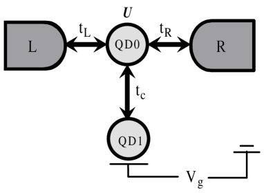
Figure 1: Schematic plot of the nanodevice. Only one quantum dot QD0 is connected with both leads. Another noninteracting quantum dot QD1 is side coupled to QD0. Energy level of QD1 can be adjusted via the gate voltage or a magnetic field.

In this paper, we systematically exploring the nonequilibrium transport properties of a T-shaped DQD where the central dot operates in the Kondo regime. The side dot is assumed to be noninteracting so that the Fano interference can be readily adjusted by changing interdot coupling and the energy level of the side dot. Current and shot noise properties of the DQD are investigated. Both Kondo effect and Fano interference play important roles in determining the transport properties of the T-shaped DQD device.

Our results were obtained by employing the slave boson mean field theory (SBMFT)PRB293035 ; PRB355072 with the use of nonequilibrium Green function following PRL851946 . The SBMFT is numerically simple and efficient for the study of transport properties in strongly correlated QDs. As a strong coupling approach, the SBMFT has been proven to be reliable for the low voltage at zero temperature. In our case, the SBMFT enables us to include nonperturbatively the interdot coupling, so that the interplay of the correlation and the interference can be explicitly studied. Due to the discrete nature of charge particles, measurement of the shot noise can reveal the correlations between carriers out of equilibriumNature392658 ; PR3361 . Unfortunately, it is usually nontrivial to obtain an expression for the shot noise of strongly correlated systems PRB71035315 ; PRL88116802 . However, such an expression is straightforward within the mean field approximation where one can apply the Wick theorem PRB71035315 ; JPCM144963 . Despite these merits, the SBMFT has its own limitations. It takes into account spin fluctuations but neglects the charge fluctuations. Therefore, calculations based on the SBMFT are restricted to the low bias limit. Otherwise, one has to rely on more advanced approaches such as the noncrossing approximation.

II model and formulation

We consider nonequilibrium transport properties of a T-shaped DQD device at zero temperature. The schematic diagram of our device is presented in Fig. 1. The central part of our device has two QDs. A single energy level is included on each dot. In our configuration, only one dot QD0 is connected to both leads via tunnelling coupling $t_{\alpha}$ ($\alpha=L,R$). There is a strong intradot Coulomb interaction $U$ on QD0. Another noninteracting dot QD1 is side coupled to QD0 via interdot tunnelling coupling $t_{c}$. The energy level of QD0 $\epsilon_{0\sigma}$ is far below the Fermi energy while the energy level of QD1 $\epsilon_{1\sigma}$ can be tuned by the external gate voltage. Here, $\sigma$ represents spin. In the following discussion, $U$ is sufficiently large ($U\rightarrow\infty$), so that double occupancy of QD0 is forbidden. The infinite $U$ slave boson language was adopted to describe the strongly correlated QD.

The Hamiltonian of our model reads:

$$H = \sum_{k\alpha,\sigma}\epsilon_{k\alpha,\sigma}c^{\dagger}_{k\alpha,\sigma}c_{k\alpha,\sigma}+\sum_{\sigma}\epsilon_{0\sigma}f^{\dagger}_{\sigma}f_{\sigma}+\sum_{\sigma}\epsilon_{1\sigma}d^{\dagger}_{\sigma}d_{\sigma}$$

$$+{{1}\over{\sqrt{N}}}\sum_{k\alpha,\sigma}t_{\alpha}(c^{\dagger}_{k\alpha,\sigma}b^{\dagger}f_{\sigma}+H.C.)$$

$$+{t_{c}\over\sqrt{N}}\sum_{\sigma}(d_{\sigma}^{\dagger}b^{\dagger}f_{\sigma}+H.C.)$$

$$+\lambda(b^{\dagger}b+\sum_{\sigma}f^{\dagger}_{\sigma}f_{\sigma}-1),$$

where $c^{\dagger}_{k\alpha,\sigma}(c_{k\alpha,\sigma})$ is the creation (annihilation) operator for an electron with spin $\sigma$ and quantum number $k$ in the $\alpha$ lead. In the slave boson representation, the creation (annihilation) operator for an electron in the $N=2$ fold degenerate QD0 with spin $\sigma$ is replaced by $f_{\sigma}^{\dagger}b\ (f_{\sigma}b^{\dagger})$ where $f_{\sigma}$ ($f^{\dagger}_{\sigma}$) is the pseudofermion operator that annihilates (creates) a singly occupied state in QD0 and $b$ ($b^{\dagger}$) is the slave boson operator which annihilates (creates) an empty state in QD0. The first line of the Hamiltonian represents electrons in the leads and the two dots. The second and third line of the Hamiltonian describes the QD0-leads tunnelling processes and the interdot coupling. The last term in the Hamiltonian with a Lagrange multiplier $\lambda$ represents the constraint $\sum_{\sigma}f^{\dagger}_{\sigma}f_{\sigma}+b^{\dagger}b=1$ for QD0 to prevent the double occupancy in the limit $U\rightarrow\infty$.

We solved this Hamiltonian by using the mean field approximation, where the boson operator is approximated by its expectation value. A real parameter $\tilde{b}$ is introduced to replace the boson operators in the Hamiltonian, namely, $b(t)/\sqrt{N}=\tilde{b}$. This approximation is exact for describing the spin fluctuation (Kondo regime) in the limit $N\rightarrow\infty$ and $T=0$. By defining the renormalization parameters $\tilde{t}_{\alpha}=t_{\alpha}\tilde{b}$, $\tilde{t}_{c}=t_{c}\tilde{b}$ and $\tilde{\epsilon}_{0\sigma}=\epsilon_{0\sigma}+\lambda$, the Hamiltonian (1) is formally reduced to the free electron model:

$$\tilde{H} = \sum_{k\alpha,\sigma}\epsilon_{k\alpha,\sigma}c^{\dagger}_{k\alpha,\sigma}c_{k\alpha,\sigma}+\sum_{\sigma}\tilde{\epsilon}_{0\sigma}f^{\dagger}_{\sigma}f_{\sigma}+\sum_{\sigma}\epsilon_{1\sigma}d^{\dagger}_{\sigma}d_{\sigma}$$

$$+\sum_{k\alpha,\sigma}\tilde{t}_{\alpha}(c^{\dagger}_{k\alpha,\sigma}f_{\sigma}+H.C.)$$

$$+{\tilde{t}_{c}}\sum_{\sigma}(d_{\sigma}^{\dagger}f_{\sigma}+H.C.)$$

$$+\lambda(N\tilde{b}^{2}-1).$$

Now, the task is to self-consistently determine the set of parameters: $\tilde{b}$ and $\lambda$. Following the Ref. PRL851946 one can first write down the constraint and the equation of motion of the slave boson operators. Thus we have two equations with the above two unknowns. Next, the two equations are closed with the nonequilibrium Green’s functions of the central dot by applying the equation of motion and the analytic continuation rules HaugJauho of the lead-dot lesser Green function. These equations in the Fourier space are given by

$$\tilde{b}^{2}-i\sum_{\sigma}\int{d\epsilon\over{4\pi}}G^{<}_{00,\sigma}(\epsilon)={1\over 2},$$ (3)

$$\lambda\tilde{b}^{2}=i\sum_{\sigma}\int{d\epsilon\over 4\pi}(\epsilon-\tilde{\epsilon}_{0,\sigma})G^{<}_{00,\sigma}(\epsilon),$$ (4)

where $G^{<}_{00,\sigma}(\epsilon)=i<f_{\sigma}^{\dagger}f_{\sigma}>$ is the lesser Green function of QD0. The retarded and the lesser Green function of QD0 are frequently used in the following calculations. These functions can be obtained by the equation of motion approach and they are given by

$$G_{00,\sigma}^{r}(\epsilon)={\epsilon-\epsilon_{1\sigma}\over(\epsilon-\tilde{\epsilon}_{0\sigma}-i\tilde{\Gamma})(\epsilon-\epsilon_{1\sigma})-\tilde{t}_{c}^{2}},$$ (5)

and

$$G_{00,\sigma}^{<}(\epsilon)={2i(\tilde{\Gamma}_{L}f_{L}(\epsilon)+\tilde{\Gamma}_{R}f_{R}(\epsilon))(\epsilon-\epsilon_{1\sigma})^{2}\over\mid(\epsilon-\tilde{\epsilon}_{0\sigma}-i\tilde{\Gamma})(\epsilon-\epsilon_{1\sigma})-\tilde{t}_{c}^{2}\mid^{2}},$$ (6)

where $f_{\alpha}$ is the Fermi distribution function in lead $\alpha$. $\tilde{\Gamma}_{\alpha}=\tilde{b}^{2}\Gamma_{\alpha}$ and $\tilde{\Gamma}=\tilde{b}^{2}\Gamma=\tilde{\Gamma}_{L}+\tilde{\Gamma}_{R}$ are the renormalized linewidth functions. The linewidth function is defined as $\Gamma_{\alpha}(\epsilon)=\pi\sum_{k\alpha,\sigma}t_{\alpha}^{2}\delta(\epsilon-\epsilon_{k\alpha,\sigma})$. In the wide band limit, $\Gamma_{\alpha}$ can be reduced to an energy-independent constant for $|\epsilon|<D$ ($D$ is the band width).

The two parameters ($\tilde{b}$ and $\lambda$) can now be self-consistently obtained by solving Eqs. (3) and (4) with the help of Eq. (6). When the side dot is decoupled to QD0, the Kondo temperature of QD0 ($\epsilon_{0}=\epsilon_{0,\sigma}$) at equilibrium is given by $T_{K}^{0}=De^{-\pi|\epsilon_{0}-E_{F}|/\Gamma}$. The self-consistently determined parameters $\tilde{\epsilon}_{0,\sigma}$ and $\tilde{\Gamma}_{\alpha}$ give exactly the position and the width of the Kondo peak in QD0.

After obtaining these parameters self-consistently, the transmission probability $T_{\sigma}(\epsilon,V_{LR})$ can be found from

$$T_{\sigma}(\epsilon,V_{LR})=G_{00,\sigma}^{a}\tilde{\Gamma}_{L}G^{r}_{00,\sigma}\tilde{\Gamma}_{R},$$ (7)

where $V_{LR}$ is the small dc voltage applied across QD0 and the advanced Green function $G^{a}$ can be calculated from the Hermite conjugate of $G^{r}$. It should be noted that comparing with the noninteracting cases, the transmission probability is a function of $V_{LR}$ due to the self-consistently determined renormalized parameters.

We studied the current and shot noise properties of the T-shaped DQD device. The current is defined as the change of electron numbers in the leads. Current noise is caused by the time-dependent fluctuation. At $T=0$, only the shot noise is nonzero while the thermal noise is fully suppressed. In deriving the shot noise expression for systems with many body interaction, a direct application of Wick theorem is not permitted due to the existence of quartic terms in the Hamiltonian. This obstacle can be circumvented by first formally reducing the quartic Hamiltonian to the quadratic form under the mean field approximation. Then, an application of the Wick theorem is straightforward. After some algebra, expressions for the current and zero frequency shot noise spectrum are given byPRL682512 ; PRB69235305

$$I={e\over h}\sum_{\sigma}\int_{0}^{eV_{LR}}d\epsilon T_{\sigma}(\epsilon,V_{LR}),$$ (8)

and

$$S={2e^{2}\over h}\sum_{\sigma}\int_{0}^{eV_{LR}}d\epsilon T_{\sigma}(\epsilon,V_{LR})(1-T_{\sigma}(\epsilon,V_{LR})),$$ (9)

where $e$ and $h$ are the charge unit and Planck constant. These results are obtained at zero temperature where the Fermi distribution function becomes a unit step function. The shot noise Fano factor $\gamma=S/2eI$ is introduced to characterize the deviation of the shot noise from the Poisson value of shot noise $2eI$.

III numerical results and discussion

In this section, we discuss the transport properties of the T-shaped DQD at zero temperature. In the following, $\Gamma$ is taken as the energy unit and $E_{F}$ at equilibrium is set to be zero as energy reference. The energy level of the central dot is fixed at $-3.5$ and the conduction band has a constant DOS with the band width $D=60$. At equilibrium and without interdot coupling, the Kondo temperature $T^{0}_{K}$ of QD0 is then approximate to be $10^{-3}$. The energy level of QD1 $\epsilon_{1}$ and the interdot coupling strength $t_{c}$ are assumed to be readily adjustable.

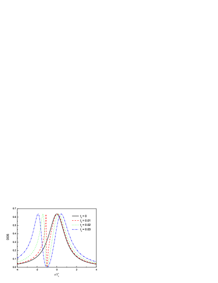
Figure 2: Density of state at QD0 $\rho_{0}$ for different coupling strength $t_{c}$. The energy level of QD1 is fixed at $-T_{K}^{0}$.

Figure 3: Differential conductance as a function of the applied voltage for various interdot couplings $t_{c}=0,0.03,0.04$ and $0.05$. The energy level of QD1 is fixed at $T^{0}_{K}$.

Let’s first calculate the local density of states (DOS) in QD0 which is given by

$$\rho_{0}(\epsilon)=-{1\over\pi}\tilde{b}^{2}\sum_{\sigma}{\rm Im}G_{00,\sigma}^{r}(\epsilon),$$ (10)

where the retarded Green function is given in Eq.(5). Fig.2 presents how the calculated local DOS at QD0 changes with the interdot coupling strength $t_{c}$. The side energy level is fixed at $-T_{K}^{0}$. The DOS without Fano interference ($t_{c}=0$) is presented for comparison. For $t_{c}=0$, the DOS shows a Breit-Wigner line shape centered at the Fermi energy. This DOS peak is solely determined by the Kondo effects. For $t_{c}\neq 0$, The Fano interference begins playing an role in complicating the DOS at QD0. The DOS profile with Fano interference presented in Fig.2 can be decomposed into a Breit-Wigner and a Fano line shape. Inserting Eq. (5) into Eq. (10) and taking into account the spin degeneracy ($\epsilon_{0\sigma}=\epsilon_{0},\epsilon_{1\sigma}=\epsilon_{1}$), the DOS expression can be written as

$$\rho_{0}(\epsilon)={2\tilde{b}^{2}\over\pi}{\tilde{\Gamma}^{2}(\epsilon-\epsilon_{1})^{2}\over(\epsilon-\epsilon_{+})^{2}(\epsilon-\epsilon_{-})^{2}+\tilde{\Gamma}^{2}(\epsilon-\epsilon_{1})^{2}},$$ (11)

where $\epsilon_{\pm}={\tilde{\epsilon}_{0}+\epsilon_{1}\over 2}\pm\sqrt{\tilde{t}_{c}^{2}+({\tilde{\epsilon}_{0}-\epsilon_{1}\over 2})^{2}}$. Eq.(11) can readily be approximated by a sum of a Breit-Wigner function and a Fano function where the details of these two functions are not presented here for simplicity. One can see that the DOS profile has two maxima at $\epsilon=\epsilon_{\pm}$. Between these two peaks, the DOS dived to zero at $\epsilon=\epsilon_{1}$. The distance between the two DOS maxima is $\epsilon_{+}-\epsilon_{-}=2\sqrt{\tilde{t}_{c}^{2}+({\tilde{\epsilon}_{0}-\epsilon_{1}\over 2})^{2}}$. The distance between the two peaks is a complex function of all the parameters of the DQD device which must be determined self-consistently. With increasing the interdot coupling $\tilde{t}_{c}$, the two peaks move to opposite directions while the zero DOS remains unchanged at the side dot energy level. When $\tilde{t}_{c}$ goes down, this distance gets smaller and the Fano peak becomes sharper. An extreme case is that as $\tilde{t}_{c}$ reaches zero, the Fano resonance width becomes zero. The Fano peak vanishes and the DOS profile reduces to the simple Breit-Wigner function.

In Fig.3, we plot the nonlinear differential conductance $dI/dV$ as a function of the applied voltage for various interdot couplings. The differential conductance is obtained by numerically differentiating Eq. (8) with respect to the bias voltage. For $t_{c}=0$, only one dot (QD0) is active. The unitary limit of the conductance at zero bias is reached due to the Kondo resonance. The differential conductance shows a zero bias anomaly which is the main feature of the differential conductance in the Kondo regime. When $t_{c}$ is nonzero, the differential conductance line shape is modified. The zero bias conductance departs from the unitary limit and the zero bias anomaly peak is suppressed with increasing interdot coupling due to the interplay of the Fano interference and the Kondo effect. When $t_{c}$ is strong enough, the zero bias anomaly eventually vanishes.

The Fano interference is dependent on not only the interdot coupling but also the side dot energy level. In Fig.4, the differential conductance as a function of the applied voltage is presented for different side dot energy level position ($\epsilon_{1}$). The interdot coupling strength is fixed at $t_{c}=0.04$. When $\epsilon_{1}$ is near the Fermi energy, the Fano interference plays an important role in weakening the Kondo resonance. One can see from Fig.4 that the zero bias anomaly for $\epsilon_{1}=0$ and $\epsilon_{1}=T^{0}_{K}$ can not survive in the parameters given above. The conductance at the zero bias is greatly reduced from the unitary limit. When $\epsilon_{1}$ is aligned with the Fermi energy ($\epsilon_{1}=0$), the conductance is zero due to the destructive interference between the Kondo resonance and the side dot level. For the case where $\epsilon_{1}$ is much higher than the Fermi energy, the Fano interference is expected to have a smaller impact on the Kondo resonance. For $\epsilon_{1}=2T^{0}_{K}$, $\epsilon_{1}=5T^{0}_{K}$ and $\epsilon_{1}=10T^{0}_{K}$, the zero bias anomaly reappears. The zero bias conductance approaches to the unitary limit.

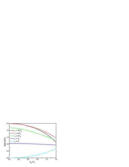
Figure 4: Differential conductance with different side dot energy levels. The interdot coupling is fixed at $t_{c}=0.04\Gamma$.

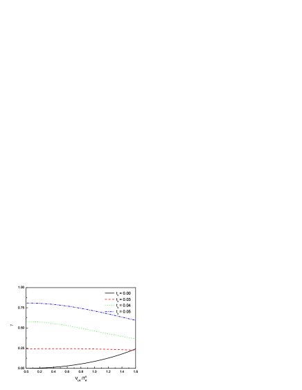
Figure 5: Bias dependence of the shot noise Fano factor $\gamma$ with different interdot coupling parameters. The side dot energy level is fixed at $\epsilon_{1}=T^{0}_{K}$.

Now, we turn to the shot noise properties of the T-shaped DQD. In Fig.5, the bias dependent Fano factor is displayed for different interdot couplings. The energy level of QD1 is fixed at $T_{K}^{0}$. We are interested in the zero bias limit Fano factor which is given by $\gamma\mid_{V_{LR}\rightarrow 0}=1-T(E_{F},0)$ according to Eq. (8) and (9). For $t_{c}=0$, QD0 acts as a perfect transparent scatterer dominated by the Kondo resonance. One can see from Fig.5 that the Kondo unitary limit leads to a complete suppression of the zero bias limit shot noise Fano factor. When the Fano interference plays its role, the Kondo resonance peak of DOS changes from a Breit-Wigner line shape to a composition of a Breit-Wigner and a Fano line shape as can be seen from Fig.2. At the same time, the zero bias conductance will depart from the unitary limit and the zero bias limit shot noise Fano factor will take on a nonzero value. This enhancement of the shot noise Fano factor can be interpreted as a result of the weakening of the DOS Kondo resonance peak at Fermi energy by the Fano interference between the two pathways through the DQD device. When $t_{c}$ becomes much stronger, The Kondo resonance at Fermi energy is destroyed by the Fano interference. The transmission probability at $E_{F}$ becomes very low. As a consequence, $\gamma$ increases very quickly and the shot noise tends to the Poisson value.

In order to check how sensitive the shot noise is to the presence of the Fano interference, we plot in Fig.6 the shot noise Fano factor $\gamma$ as a function of $t_{c}$ at fixed $V_{LR}$ ($V_{LR}=T^{0}_{K}$) for different $\epsilon_{1}$. It is shown in Fig.6 that the shot noise Fano factor with $\epsilon_{1}$ near $E_{F}$ is more sensitive to the interdot coupling than that where $\epsilon_{1}$ is far from $E_{F}$. For cases where $\epsilon_{1}$ is near the Fermi energy ($\mid\epsilon_{1}-E_{F}\mid<T_{K}^{0}$), the Kondo resonance peak at Fermi energy will be abruptly quenched by the emergence of the Fano interference. This leads to a sudden increase of $\gamma$ from a small value at zero interdot coupling to the Poisson value. Therefore, the Fano factor $\gamma$ is highly sensitive to the interdot coupling when $\epsilon_{1}$ is near the Fermi energy as shown in Fig.6. On the contrary, for cases where $\epsilon_{1}$ is far from the Fermi energy ($\mid\epsilon_{1}-E_{F}\mid\gg T_{K}^{0}$), $\gamma$ will be less sensitive to the interdot coupling strength. This is because the presence of interdot coupling is expected to have a weaker destructive interference on the Kondo resonance peak of DOS at $E_{F}$. On can see from Fig.6, for a larger $\epsilon_{1}$, $\gamma$ keeps to be small over a wider range of the tunable interdot coupling before it rises to the Poisson limit. One may also found from Fig.6 that $\gamma$ will show a non-monotonic relation with $t_{c}$ at finite bias. It is interesting that the minimum of the shot noise Fano factor is not obtained at the zero interdot coupling where the Kondo resonance dominates the transport properties. This can be best seen when $\mid\epsilon_{1}\mid\gg T_{K}^{0}$ where $\gamma$ first decreases with increasing $t_{c}$ when $t_{c}$ is below a critical value and then increase quickly with $t_{c}$ to reach the Poisson value. For a larger $\epsilon_{1}$, one can see from Fig. 6 that this value moves to the strong interacting end. This critical value is a function of the side dot energy level and the applied bias. It is nontrivial to obtain an analytical expression for the critical value because all the parameters in the Kondo regime have to be determined self-consistently. This non-monotonic behavior of $\gamma$ is due to the interplay of the Fano interference and the Kondo effects. The critical value stands for the situation where the coherent transport is optimized as the competition of the Kondo effects and Fano interference.

IV summary

In this work, we presented the transport properties of a T-shaped DQD device where the central dot is in the Kondo regime. We solved this problem by using the SBMFT at low bias voltage and zero temperature. When the side dot is decoupled, the Kondo resonance in the central dot results in the unitary limit of the linear conductance and the zero bias anomaly. The shot noise Fano factor at zero bias is fully suppressed to zero. It is more interesting to study the case where a side dot can interact with the central dot. When an electron is emitted from one lead, there is quantum interference between two electron waves, one directly passing through the central dot and one traveling through the two dots, before the electron arrives at the other lead. This Fano interference can act to weaken the Kondo resonance at the Fermi energy. The DOS is composed of Breit-Wigner and Fano line shapes. As a consequence, the linear conductance will depart from the unitary limit and the zero bias anomaly will be suppressed in the presence of interdot coupling. The zero bias anomaly will eventually vanishes at large interdot coupling strength or the side dot energy is tuned near the Kondo resonance peak. The zero bias shot noise Fano factor increases with the interdot coupling and tends to the Poisson value. Detailed study indicates that at finite bias, the shot noise Fano factor shows a non-monotonic behavior with the interdot coupling strength as a result of the interplay of the Kondo effect and the Fano interference.

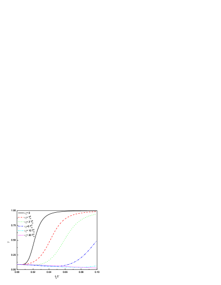
Figure 6: Fano factor as a function of the interdot coupling strength for different $\epsilon_{1}$. The bias is fixed at $V_{LR}=T_{K}^{0}$.

- (1) A. C. Hewson, The Kondo Problem to Heavy Fermions (Cambridge University Press, Cambridge, 1993).
- (2) T. K. Ng and P. A. Lee, Phys. Rev. Lett. , 1768 (1988).
- (3) S. Hershfield, J. H. Davies, and J. W. Wilkins, Phys. Rev. Lett. , 3720 (1991).
- (4) Y. Meir, N. S. Wingreen, and P. A. Lee, Phys. Rev. Lett. , 2601 (1993).
- (5) W. G. van der Wiel, S. De Franceschi, J. M. Elzerman, T. Fujisawa, S. Tarucha, and L. P. Kouwenhoven, Rev. Mod. Phys. , 1 (2003).
- (6) A. Georges, and Y. Meir, Phys. Rev. Lett. , 3508 (1999).
- (7) H. Jeong, A. M. Chang, and M. R. Melloch, Science , 2221 (2001).
- (8) R. Aguado and D. C. Langreth, Phys. Rev. Lett. , 1946 (2000).
- (9) T. Aono and M. Eto, Phys. Rev. B , 125327 (2001).
- (10) D. Boese, W. Hofstetter, and H. Schoeller, Phys. Rev. B , 125315 (2002).
- (11) R. López, R. Aguado, and G. Platero, Phys. Rev. B , 235305 (2004).
- (12) T. S. Kim and S. Hershfield, Phys. Rev. B ,245326 (2001).
- (13) P. S. Cornaglia and D. R. Grempel, Phys. Rev. B , 075305 (2005).
- (14) M. L. L. de Guevara, F. Claro, and P. A. Orellana, Phys. Rev. B , 195335 (2003).
- (15) B. R. Bulka and P. Stefański, Phys. Rev. Lett. , 5128 (2001).
- (16) W. Hofstetter, J. König, and H. Schoeller, Phys. Rev. Lett. , 156803 (2001).
- (17) A. C. Johnson, C. M. Marcus, M. P. Hanson, and A. C. Gossard, Phys. Rev. Lett. , 106803 (2004).
- (18) K. Kang, S. Y. Cho, J. J. Kim, and S. C. Shin, Phys. Rev. B , 113304 (2001).
- (19) M.E.Torio, K. Hallberg, A. H. Ceccatto, and C. R.Proetto, Phys. Rev. B , 085302 (2002).
- (20) A. Golub and Y. Avishai, Phys. Rev. B , 165325 (2004).
- (21) B. H. Wu and J. C. Cao, J. Phys.:Condens. Matter 16, 8285 (2004).
- (22) P. Coleman, Phys. Rev. B 29, 3035 (1984).
- (23) P. Coleman, Phys. Rev. B 35, 5072 (1987).
- (24) R. Landauer, Nature 392, 658 (1998).
- (25) Y. M. Blanter and M. Büttiker, Phys. Rep. 336, 1 (2002).
- (26) D. Sánchez and R. Löpez, Phys. Rev. B 71, 035315 (2005).
- (27) Y. Meir and A. Golub, Phys. Rev. Lett. 88, 116802 (2002).
- (28) B. Dong and X. L. Lei, J. Phys.: Condens. Matter 14, 4963 (2002).
- (29) H. Haug and A.-P. Jauho, Quantum Kinetics in Trans-port and Optics of Semiconductors (Springer-Verlag, Berlin, 1998).
- (30) Y. Meir and N. S. Wingreen, Phys. Rev. Lett. 68, 2512 (1992).