Disorder, spin-orbit, and interaction effects in dilute ${\rm Ga}_{1-x}{\rm Mn}_{x}{\rm As}$

Abstract

We derive an effective Hamiltonian for ${\rm Ga}_{1-x}{\rm Mn}_{x}{\rm As}$ in the dilute limit, where ${\rm Ga}_{1-x}{\rm Mn}_{x}{\rm As}$ can be described in terms of spin $F=3/2$ polarons hopping between the Mn sites and coupled to the local Mn spins. We determine the parameters of our model from microscopic calculations using both a variational method and an exact diagonalization within the so-called spherical approximation. Our approach treats the extremely large Coulomb interaction in a non-perturbative way, and captures the effects of strong spin-orbit coupling and Mn positional disorder. We study the effective Hamiltonian in a mean field and variational calculation, including the effects of interactions between the holes at both zero and finite temperature. We study the resulting magnetic properties, such as the magnetization and spin disorder manifest in the generically non-collinear magnetic state. We find a well formed impurity band fairly well separated from the valence band up to $x_{\rm active}\lesssim 0.015$ for which finite size scaling studies of the participation ratios indicate a localization transition, even in the presence of strong on-site interactions, where $x_{\rm active}<x_{\rm nom}$ is the fraction of magnetically active Mn. We study the localization transition as a function of hole concentration, Mn positional disorder, and interaction strength between the holes.

I Introduction

Recently there has been a surge of interest in the more than 30 year old field of diluted magnetic semiconductorsrev that has been largely motivated by the potential application of these materials in spin-based computationDiVincenzo (1995); Nielson and Chuang (2000); Awschalom et al. (2002); Zutic et al. (2004) devices. In particular, the discovery of ferromagnetism in low-temperature molecular beam epitaxy (MBE) grown ${\rm Ga}_{1-x}{\rm Mn}_{x}{\rm As}$ has generated renewed interest.Ohno (1998) In this material Curie temperatures as high as $T_{c}\approx 160{\rm K}$ have been observed.Edmonds et al. (2004)

In this paper we focus on one of the most studied magnetic semiconductors, ${\rm Ga}_{1-x}{\rm Mn}_{x}{\rm As}$, though most of our calculations carry over to other p-doped III-V magnetic semiconductors. In ${\rm Ga}_{1-x}{\rm Mn}_{x}{\rm As}$ substitutional ${\rm Mn}^{2+}$ play a fundamental role: They provide local spin $S=5/2$ moments and they dope holes into the lattice.Linnarsson et al. (1997) Since the ${\rm Mn}^{2+}$ ions are negatively charged compared to ${\rm Ga}^{3+}$, in the very dilute limit they bind these holes forming an acceptor level with a binding energy $E_{b}\approx 112{\rm meV}$. Linnarsson et al. (1997) As the ${\rm Mn}$ concentration increases, these acceptor states start to overlap and form an impurity band, which for even larger ${\rm Mn}$ concentrations merges with the valence band. Though the actual concentration at which the impurity band disappears is not known, according to optical conductivity measurements,Singley et al. (2002, 2003) and ellipsometryBurch et al. (2004) this impurity band seems to persist up to nominal ${\rm Mn}$ concentrations as high as $x_{\rm nom}\approx 0.05$. Angle resolved photoemission (ARPES) data,Asklund et al. (2002); Okabayashi et al. (2001a, b) scanning tunneling microscope (STM) resultsGrandidier et al. (2000); Tsuruoka et al. (2002) and the fact that even “metallic” samples feature a resistivity upturn at low temperatureEsch et al. (1997) suggest that for smaller concentrations (and maybe even for relatively large nominal concentrations) one may be able to describe ${\rm Ga}_{1-x}{\rm Mn}_{x}{\rm As}$ in terms of an impurity band.Fiete et al. (2003); Berciu and Bhatt (2001); Kennett et al. (2002a); Zhou et al. (2004) While optical conductivity resultsSingley et al. (2002, 2003) and ellipsometry resultsBurch et al. (2004) are suggestive of the presence of an impurity band in moderately doped samples,Singley et al. (2002, 2003) an interpretation based on band to band transitions is also possible.Hankiewicz et al. (2004) We remark, however, that these materials are extremely dirtyTimm et al. (2002)–the mean free path is estimated to be of the order of the Fermi wavelength–and therefore it is not clear if the latter approach is appropriate. Also, ARPES data indicate that the chemical potential of “insulating” samples lies inside the gap,Asklund et al. (2002) contradicting a band theory-based interpretation of the optical conductivity data.

A detailed understanding of an impurity band model begins with the knowledge of a single Mn acceptor state.Mahadevan and Zunger (2004) The physics of the isolated ${\rm Mn}^{2+}$ + hole system is well understood: Linnarsson et al. (1997) In the absence of the $\rm{Mn}^{2+}$ core spin, the ground state of the bound hole at the acceptor level is four-fold degenerate and well described in terms of a $F=3/2$ state. For most purposes, only the fourfold degenerate $F=3/2$ acceptor levels need be considered in the dilute limit even in the presence of the $\rm{Mn}^{2+}$ core spin. As evidenced by infrared spectroscopy, Linnarsson et al. (1997) the effect of the $S=5/2$ ${\rm Mn}$ core spin on the holes is well-described by a simple exchange Hamiltonian:rev

$$H_{\rm exch}=G{\vec{S}}\cdot{\vec{F}}\;,$$ (1)

with $G\approx 5$ meV. Linnarsson et al. (1997)

The bound hole (acceptor) states within the $F=3/2$ multiplet are not Hydrodgenic due to a significant d-wave component of the bound state wavefunction.Fiete et al. (2003); Tang and Flatté (2004); Averkiev and ll’inski (1994); Baldereschi and Lipari (1973) This d-wave character ultimately comes from the spin-orbit coupling in GaAs and has recently been confirmed in the beautiful STM experiments of Yakunin et. al.Yakunin et al. (2004) The anistropy of the orbital structure of the wavefunction leads to directionally dependent hopping of holes between Mn ions, a splitting of the $F=3/2$ level degeneracy, and is expected to strongly influence the magnetic and transport properties of dilute GaMnAs.Fiete et al. (2003) Here we study these effects in detail.

One of the main results of this paper is thus the effective Hamiltonian describing strongly interacting holes hopping from Mn to Mn. The holes are coupled to the Mn spins via the exchange interaction (1), where

$$H^{\rm eff}=H_{0}^{\rm eff}+H_{\rm int}\;.$$ (2)

The first part of this Hamiltonian, $H_{0}^{\rm eff}$, describes the hopping of the holes from Mn to Mn, and the interactions of the Mn acceptor site with the Mn core spin,

$$H_{0}^{\rm eff} = \sum_{(i,j)}c^{\dagger}_{i,\mu}t^{\mu\nu}_{ij}c_{j,\nu}+\sum_{i}c^{\dagger}_{i,\mu}\;(K_{i}^{\mu\nu}+E_{i}\;\delta^{\mu\nu})\;c_{i,\nu}$$ (3)

$$+ G\sum_{i,\mu,\nu}{\vec{S}}_{i}\cdot(c_{i,\mu}^{\dagger}{\vec{F}}^{\mu\nu}\;c_{i,\nu})\;.$$

To determine the parameters of (3) we shall use the spherical approximation.Baldereschi and Lipari (1973) This approach neglects the cubic symmetry of the lattice, but approximates the band structure rather well around the top of the valence band at the Gamma point which is most relevant at the low hole concentrations of interest in the present paper. The term $H_{\rm int}$ accounts for the on-site interactions of holes with each other, and in the spherical approximation,

$$H_{\rm int}={U_{N}\over 2}\sum_{i}:{{\hat{N}}_{i}}^{2}:+{U_{F}\over 2}\sum_{i}:{\hat{\vec{F}}^{2}}_{i}:\;.$$ (4)

The operator $c^{\dagger}_{i,\nu}$ in the above expressions creates a hole at the acceptor level $|F=3/2,F_{z}=\nu\rangle$ at site $i$, ${\hat{N}}_{i}=\sum_{\nu}c^{\dagger}_{i,\nu}c_{i,\nu}$, ${\hat{\vec{F}}}_{i}=\sum_{\mu,\nu}c^{\dagger}_{i,\mu}{\vec{F}}^{\mu\nu}c_{i,\nu}$, and $:...:$ denotes normal ordering. Here ${\vec{F}}^{\mu\nu}$ is the $\mu\nu$ element of the spin 3/2 matrix. The Hubbard interaction strength $U_{N}$ and the Hunds rule coupling $U_{F}$ in Eq. (4) can be obtained by evaluating exchange integrals and we find $U_{N}\approx 2600$ K and $U_{F}\approx-51$ K.

The presence of nearby $\rm Mn$ sites has three important effects on the $F=3/2$ acceptor state at any particular $\rm Mn$ site: (i) The Coulomb potential of the neighboring ${\rm Mn}^{2+}$ ions induces a random (from the random relative positions of the Mn) shift $E$ of the fourfold degenerate states. (ii) Because of the large spin-orbit coupling in GaAs, the neighboring atoms also generate an anisotropy $K$ and split the fourfold degeneracy of the $F=3/2$ state into two Kramers degenerate doublets. (iii) Finally, the presence of the neighboring ions allow these $F=3/2$ spin objects to hop between the ${\rm Mn}$ sites. However, this hopping $t$ does not conserve the spin $F$ because of the spin-orbit coupling.

To determine the parameters of (3), we performed variational calculations for a dimer of Mn ions taken to lie along the z-axis where $F_{z}$ is good quantum number. Once the parameters of the dimer is in hand and the positions of all the Mn are known, the parameters of the Hamiltonian (3) are obtained by simple spin-3/2 rotations.

To illustrate the power of the approach, and to better understand the physical results we obtain from it, consider the simplest case of 2 Mn impurities and 1 hole. Diagonalizing Eq. (3) for different orientations of ${\vec{S}}_{1}$ and ${\vec{S}}_{2}$ with the parameters given in Fig. 4 shows that the magnetization has an easy axis anisotropy (See Fig. 1). This easy axis anisotropy immediately leads to frustration among non-collinear Mn positions.

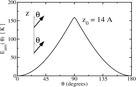
Figure 1: Spin orientation dependence of the ground state energy of one hole on a Mn dimer parallel to the z-axis for a spatial separation of $z_{0}=14$ Å. The Hamiltonian (3) is diagonalized exactly with the parameters shown in Fig. 4. As the spins are rotated by an angle $\theta$ away from the z-axis the energy increases and reaches a maximum at $\theta=90^{o}$ before again decreasing. This indicates the magnetic anisotropy is easy axis.

We study the Hamiltonian $H^{\rm eff}=H_{0}^{\rm eff}+H_{\rm int}$ in detail using mean field theory when $U_{N}=U_{F}=0$ and also with a variational approach when $U_{N},U_{F}\neq 0$. We study the interplay of disorder and directionally dependent hopping parameters induced by spin-orbit coupling. We calculate the temperature dependence of the magnetization, magnetic anisotropies, the spin distribution functions measuring the degree of non-collinearity among the spins, the (impurity band) density of states, and the dependence of the localization transition on the various parameters of our model. Our main results are the following: Qualitatively similar to our earlier results in the metallic regime,Zaránd and Jankó (2002); Fiete et al. (2005) we find that the interplay of disorder and spin-orbit coupling results in (i) magnetization curves that exhibit linear behavior over a significant temperature range and (ii) a broad spin distribution function, implying highly non-collinear magnetic states that result from spin-orbit induced magnetic anisotropies (iii) within our mean field and variational calculation we find a well developed impurity band separated from the valence band for active Mn concentration up to $x_{\rm active}\lesssim 0.015$ with a localization transition fairly robust to interactions.

In this paper all Mn concentrations $x$ are the active Mn concentrations, i.e., $x=x_{\rm active}$ where active Mn are defined to be those Mn that contribute to the ferromagnetism of the material. Interstitial defects with a Mn sitting next to a substitutional Mn may result in a local singlet formation,Bergqvist et al. (2003) thereby rendering the two Mn magnetically inactive since they do not contribute to the ferromagnetism of the material. Thus, the active Mn concentration is typically less than the nominal Mn concentration.

The interstitial Mn also compensate holesEdmonds et al. (2004); Yu et al. (2002a) reducing the number of itinerant holes. In this paper we use the hole fraction $f$, to relate the hole to the Mn concentration as $N_{h}=f\,N_{Mn}$ where $N_{h}$ is the number of holes and $N_{Mn}$ is the number of active Mn. Although the precise value of $f$ is not known, typically, $f=0.1-0.3$. We thus include the effects of various compensating defects,Timm et al. (2002); Tim (a); Fiete et al. (2005); Potashnik et al. (2001); Yu et al. (2002b); Hayashi et al. (2001) such as interstitial Mn and As antisites indirectly through the parameter $f$.

The outline of this paper is the following. In Sec. II we describe the variational calculation used to obtain an estimate of the bound state acceptor wavefunction around a single Mn ion. In Sec. III we use the variationally obtained wavefunctions to derive and compute the effective parameters of the Hamiltonian, Eqs.(3) and (4), which we then study in detail in Sec. IV using mean field and variational approaches. Finally, in Sec. V we discuss the main conclusions of our work. Technical details of our calculations and various lengthy analytical expressions are relegated to the appendices.

II Variational Calculation of the Baldereschi-Lipari Wavefunctions

In order to study GaMnAs in the dilute limit, we proceed stepwise by first obtaining bound state (acceptor) wavefunctions in the single substitutional Mn impurity limit and then using these wavefunctions to obtain effective parameters of two-ion and $N$-ion Hamiltonians, details of which are given in Sec. III.

We start from the spherical HamiltonianBaldereschi and Lipari (1973); Zaránd and Jankó (2002); Fiete et al. (2005)

$$H_{0}^{\rm ion}={\gamma\over 2m}\Bigl{(}p^{2}-\mu\sum_{\alpha,\beta}J_{\alpha\beta}p_{\alpha\beta}\Bigr{)}-{e^{2}\over\epsilon\;r}+V_{cc}(r)\;,$$ (5)

where the central cell correctionYang and MacDonald (2003); Bhattacharjee and á la Guillaume (2000)

$$V_{cc}=-V_{0}e^{-({r\over r_{0}})^{2}}\;,$$ (6)

is used to reproduce the experimentally obtained binding energies, and therefore reasonable acceptor wavefunctions. This affects the parameters given in Fig. 4 of the effective Hamiltonian (3). Here $r_{0}$ is a short distance cutoff for the central cell correction and $V_{0}$ its size. The primary role of the central cell correction (6) is to take into account atomic interactions in the close vicinity of the Mn ion. In Eq. (5) $\gamma\approx 7.65$ is a mass renormalization parameter, $m$ is the free electron mass, $\mu\approx 0.77$ is the strength of the spherical spin-orbit coupling in the $j=3/2$ band of GaAs,Baldereschi and Lipari (1973) and $\epsilon\approx 10$ is the dielectric constant of GaAs. The spin-orbit term in Eq. (5) couples the momentum tensor of the holes $p_{\alpha\beta}=p_{\alpha}p_{\beta}-\delta_{\alpha\beta}\;p^{2}/3$ to their quadrupolar momentum, $J_{\alpha\beta}=(j_{\alpha}j_{\beta}+j_{\beta}j_{\alpha})/2-\delta_{\alpha\beta}\;j(j+1)/3$. This effective Hamiltonian gives a relatively accurate value of the hole energy in the vicinity of the top of the valence band, but is not very reliable for holes with higher energy, since then other states not included in the derivation of (5) will be mixed into the acceptor state wave functions. The Hamiltonian (3) also does not distinguish between different crystalline directions. We will discuss the implications of these features and other shortcomings of the spherical approximation in the concluding section, Sec. V.

To proceed with the calculation, we note that Eq. (5) can be made dimensionless by measuring distance in units of the effective Bohr radius, $a_{\rm eff}=\hbar^{2}\epsilon\gamma/e^{2}m=40\AA$, and taking the corresponding effective Rydberg, $R_{\rm eff}=e^{4}m/2\hbar^{2}\epsilon^{2}\gamma=15.7$meV, as the energy scale. In our calculations we have used $r_{0}=2.8\AA$ and $V_{0}=3.0$ eV. These values are very close to the numbers used for the central cell corrections in Ref.[Bhattacharjee and á la Guillaume, 2000] and Ref.[Yang and MacDonald, 2003].

With the central cell correction, we obtain the correct binding energy of 112 meV.Linnarsson et al. (1997) However, due to the central cell correction (6), $a_{\rm eff}$ is no longer a measure of the spatial extent of the wavefunction as it would be for a purely Coulomb potential. Instead, the characteristic length scale is $\sim 10\AA$, as can be seen in Fig. 2.

When $\mu\neq 0$ in Eq. (5), the ground state of a hole bound to an acceptor is no longer a state of zero orbital angular momentum, $L=0$, since the “spin-orbit” term will mix in a $d$-wave, $L=2$, component.Baldereschi and Lipari (1973) The ground state wavefunction is therefore no longer Hydrogenic and hence not spherically symmetric.Fiete et al. (2003); Averkiev and ll’inski (1994); Yakunin et al. (2004) This feature will lead directly to the appearance of spin-dependent hopping terms in Eq. (3).

Within the spherical approximation, the total angular momentum $\vec{F}=\vec{L}+\vec{j}$ is a constant of the motion and for $\mu\neq 0$ and the ground state has $F=3/2$. The wavefunction for the ground state can then be written as a sum of an $s$-wave component $f_{0}$ and a $d$-wave component $g_{0}$

$$\Phi_{F_{z}}(\vec{r}) = f_{0}(r)|L=0,j={3\over 2},F=\frac{3}{2},F_{z}\rangle$$ (7)

$$+ g_{0}(r)|L=2,j={3\over 2},F={3\over 2},F_{z}\rangle\;.$$

By acting with the Hamiltonian, Eq. (5), on Eq. (7) one obtains the following set of differential equations to be solved for $f_{0}(r)$ and $g_{0}(r)$:

$$\pmatrix{-{1\over r}{d^{2}\over dr^{2}}r-{2\over r}+\tilde{V}_{cc}&\mu\left({d^{2}\over dr^{2}}-{1\over r}{d\over dr}\right)\cr\mu\left({d^{2}\over dr^{2}}-{1\over r}{d\over dr}\right)&-{1\over r}{d^{2}\over dr^{2}}r+{6\over r^{2}}-{2\over r}+\tilde{V}_{cc}}\pmatrix{f_{0}(r)\cr g_{0}(r)\cr}=E_{0}\pmatrix{f_{0}(r)\cr g_{0}(r)\cr}\;,$$ (8)

where $\tilde{V}_{cc}\equiv\frac{2ma_{eff}^{2}}{\hbar^{2}\gamma}V_{cc}$. In order to solve Eq. (8) we follow the variational approach of Ref. [Baldereschi and Lipari, 1973] by expanding $f_{0}$ and $g_{0}$ as

$$f_{0}(r) = \sum_{i=1}^{N}A_{i}\;f_{i}(r)\;,$$ (9)

$$g_{0}(r) = \sum_{i=1}^{N}B_{i}\;g_{i}(r)\;,$$ (10)

where the $A_{i}$ and $B_{i}$ are variational parameters to be determined and the $f_{i}(r)$ and $g_{i}(r)$ are normalized but not orthogonal basis functions

$$f_{i}(r) = \frac{2\sqrt{2}\alpha_{i}^{3/4}}{\root 4 \of{\pi/2}}e^{-\alpha_{i}r^{2}}\;,$$ (11)

$$g_{i}(r) = r\frac{4\sqrt{2}\alpha_{i}^{5/4}}{\sqrt{3}\root 4 \of{\pi/2}}e^{-\alpha_{i}r^{2}}\;,$$ (12)

with $\alpha_{i}=g^{i-1}\alpha$. In our computations we have taken $N=21$, $\alpha=1\times 10^{-2}$, and $\alpha_{N}=5\times 10^{5}$ as in Ref. [Baldereschi and Lipari, 1973], and we also verified that refining the basis set resulted in no further improvement.

To obtain the ground state wave function, we minimize the expectation value of the Hamiltonian on the left hand side of Eq. (8). Using the coefficients $A_{i}$ and $B_{i}$ as variational parameters this involves the solution of a simple $2N\times 2N$ eigenvalue problem. One must, however, also take into account during this calculation that the states $f_{i}$ and $g_{i}$ are not orthogonal.

The non-orthogonality of the basis set can be taken into account through the computation of the overlap matrices, $S^{f}_{ij}=\int_{0}^{\infty}dr\;r^{2}f_{i}(r)\;f_{j}(r)$ and $S^{g}_{ij}=\int_{0}^{\infty}dr\;r^{2}g_{i}(r)\;g_{j}(r)$, and the transformation of the original problem to a corresponding new orthonormal basis following rather standard atomic physics procedures. The radial functions $f_{0}(r)$ and $g_{0}(r)$ obtained in this way are shown in Fig. 2. Note that while the $s$-wave component $f_{0}$ dominates at short distances, the $d$-wave component $g_{0}$ becomes appreciable for $r>10\AA$. This $d$-wave component is ultimately responsible for the strong anisotropy of the hopping and effective spin-spin interaction.

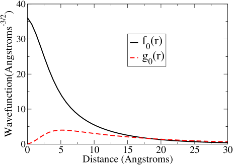
Figure 2: (Color online.) Radial wavefunctions obtained from a variational calculation for $\mu=0.767$, the relevant value for GaMnAs. For $r\gtrsim 15\AA$, the typical Mn-Mn distance at $x=0.01$, $g_{0}(r)\approx f_{0}(r)$. From Eq. (7) this means the d-wave component of the wavefunction is important for typical Mn concentrations at $x=0.01$. It is thus expected that the non-Hydrogenic nature of the wavefunction will strongly affect the magnetic and transport properties of dilute GaMnAs, a result supported by our numerical calculations presented in Sec. IV.

Using the radial wavefunctions plotted in Fig. 2 one can compute the expectation value of the local spin density, $\langle\vec{j}({\bf r})\rangle$, around a Mn impurity. Replacing the Mn spin for a moment with a classical spin pointing downward along the $z$-axis, a bound hole on the acceptor level will occupy the state $F_{z}=3/2$, provided that the coupling between the Mn spin and the hole is antiferromagnetic. The spin direction (polarization) of this bound hole around the impurity is shown in Fig. 3. Note that the polarization direction depends on distance and can change sign. Note also that in the absence of spin-orbit coupling, $\mu=0$, the spin polarization of the hole would be just pointing along the $z$ direction, and display RKKY oscillations at larger distances (not shown in the figure). Detailed expressions for the acceptor state spin density are given in Appendix A.

Figure 3: Polarization of a bound hole in the state $|F=3/2,F_{z}=3/2\rangle$ in $\rm Ga_{1-x}Mn_{x}As$ around a Mn ion (dark arrow pointing downward represents the Mn S=5/2 spin). Only the direction of the polarization is indicated. The magnitude falls off on a scale $\sim 10$ Å, as indicated by Fig. 2.

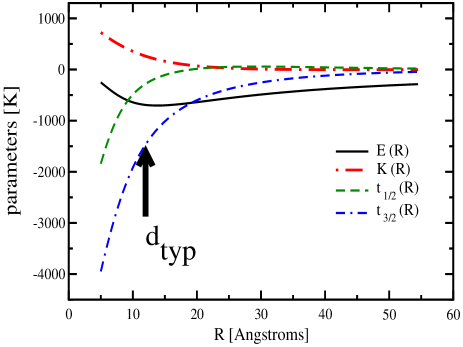
Figure 4: (Color online.) Parameters of the two-impurity Hamiltonian Eq. (15) obtained from the variational study of two Mn ions. The arrow indicates the typical Mn-Mn distance, $d_{\rm typ}$, for $x=0.01$ Mn concentration.

III Computing the two-ion and $N$-ion Hamiltonian

Using the variational wave function obtained in Sec. II, Eq. (7), we now compute the effective parameters of the two-ion hopping Hamiltonian, Eq. (15), which will in turn allow us to find the parameters of the $N$-ion Hamiltonian, Eq. (3), by using spin-3/2 rotations.

We assume that we have two impurities separated by a distance $R$. We take the quantization axis, $z$, to be along the line joining the two impurities (ions). Neglecting again the effect of the core Mn spin (for the time being), the full Hamiltonian within the spherical approximation can be written as

$$H_{0}^{2-\rm ion}={\gamma\over 2m}\Bigl{(}p^{2}-\mu\sum_{\alpha,\beta}J_{\alpha\beta}p_{\alpha\beta}\Bigr{)}+V_{1}({\vec{r}})+V_{2}({\vec{r}})\;,$$ (13)

where

$$V_{i}({\vec{r}})=-{e^{2}\over\epsilon\;|\vec{r}-\vec{r}_{i}|}+V_{cc}(|\vec{r}-\vec{r}_{i}|),$$ (14)

with $\vec{r}_{1}$ and $\vec{r}_{2}$ the locations of the two impurities.

Having computed the single ${\rm Mn}$ hole states, we carried out a variational calculation to construct the molecular orbitals for a pair of ${\rm Mn}$ ions in the approximation where we considered only linear combinations of the single impurity ground state wave functions.Fiete et al. (2003); Durst et al. (2002) For a pair of Mn spins the full SU(2) symmetry of the single impurity model is broken. However, the Hamiltonian (13) still possesses a cylindrical symmetry, corresponding to the conservation of $F_{z}$. As a consequence, the various $F_{z}$ subspaces decouple, and our task reduces to the construction and diagonalization of $2\times 2$ matrices. Furthermore, time reversal symmetry implies that the two states with $F_{z}=\pm 1/2$ and the two states with $F_{z}=\pm 3/2$ remain degenerate. As a consequence, we find that the two four-fold degenerate $F=3/2$ acceptor states of the two Mn impurities are split into four Kramers degenerate doublets. (Details of this calculation are given in Appendix B.) Since for typical Mn distances these orbitals are well separated from the rest of the spectrum, we shall be satisfied by providing a description of only these eight lowest lying states of the “molecule”. This can be achieved by using the following effective Hamiltonian:

$$H^{\rm eff}_{{\rm Mn}-{\rm Mn}}=\sum_{\nu}t_{\nu}(R)\left(c^{\dagger}_{1,\nu}c_{2,\nu}+{\rm h.c.}\right)$$ (15)

$$\phantom{mm}+\sum_{\scriptstyle i=1,2\atop\scriptstyle\nu}\left(K(R)\;\left(\nu^{2}-{5\over 4}\right)+E(R)+E_{0}\right)\;c^{\dagger}_{i,\nu}c_{i,\nu}\;,$$

where $R=|{\vec{r}_{1}}-{\vec{r}_{2}}|$, $t_{\nu}$ describes the hopping of $F_{z}=\nu$ holes, $K$ is the splitting of the $F=3/2$ manifold of states generated by the presence of the other Mn impurity, and $E$ denotes the energy shift of the acceptor state (at one ion due to the presence of the other ion) with respect to the binding energy of an isolated acceptor, $E_{0}\approx 112\;{\rm meV}$. By time reversal symmetry, the hopping parameters satisfy $t_{3/2}=t_{-3/2}$ and $t_{1/2}=t_{-1/2}$. All parameters depend only on the distance $R$ between the two Mn sites (see Fig. 4). The most obvious effect of the spin-orbit coupling is that the hoppings $t_{3/2}$ and $t_{1/2}$ substantially differ from each other; holes that have their spin aligned with the Mn-Mn bond are more mobile. As we mentioned in the introduction, this leads to an easy axis magnetic anisotropy in the effective spin-spin interactions and to non-collinear magnetism. As indicated by the arrow in Fig. 4, at the typical Mn-Mn distance for $x=0.01$, $K$ and $t_{1/2}$ can be entirely neglected compared to $E$ and $t_{3/2}$. Therefore, in many cases it is enough to keep only the latter two terms in the effective Hamiltonian.

So far, we have neglected the interaction between the core Mn spins $S$ and the acceptor state. It is known from experiments,Linnarsson et al. (1997) that the spectrum of an isolated Mn impurity can be very well described by a simple exchange Hamiltonian, $H_{\rm exch}=G\;\vec{S}\cdot\vec{F}$. Furthermore, the separation $\sim 100\;{\rm meV}$ of the acceptor state from other excited states is much smaller than the experimentally found exchange coupling $G\approx 5\;{\rm meV}$. We can therefore safely treat the exchange field of the Mn spin as a perturbation. We remark at this point that the Mn ions are, to a very good approximation, in a $d^{5}$ state, and valence fluctuations on the $d$-levels seem to be rather small, as evidenced by an experimentally observed $g$-factor close to 2.Linnarsson et al. (1997) In this spirit, we take into account the effect of Mn core spins through the following simple term,

$$H_{\rm exch}=G\sum_{i=1,2}\sum_{\mu,\nu}{\vec{S}}_{i}\cdot(c_{i,\mu}^{\dagger}{\vec{F}}^{\mu\nu}\;c_{i,\nu})\;.$$ (16)

Note that in this expression we neglected interactions between the core spins and the hole spin on a neighboring Mn acceptor level. This approximation is certainly justified in the extreme dilute limit, and the above Hamiltonian does give a reasonable value for the Curie temperature at the concentrations we consider. However, additional terms may be important for a quantitative description of GaMnAs.Mahadevan and Zunger (2004)

Finally, let us discuss the hole-hole interaction term, Eq. (4). Again, the on site interaction can be greatly simplified due to the presence of SU(2) symmetry within the spherical approximation. Since holes are fermions, two holes can be placed to the four lowest lying acceptor states in six different ways. These six states correspond to a fivefold degenerate total spin $F=F_{1}+F_{2}=2$ two-hole state and an $F=0$ singlet state. The interaction term can be thus written as

$$H_{\rm int}=U_{D}\;P_{D}+U_{S}\;P_{S}\;,$$ (17)

where we introduced the four Fermion operators $P_{D}$ and $P_{S}$ that project to the $F=2$ and $F=0$ two-hole subspaces, respectively. With a little algebra we can rewrite these expressions in the form Eq. (4), and we can express the Hubbard interaction $U_{N}$ and the Hund’s rule coupling $U_{F}$ in terms of simple Coulomb integrals (see Appendix C for details).

In the more general case, with three or more impurities, we need to know how to generalize the Hamiltonian (15) to the situation where the impurities do not lie along the $z$-axis. We can derive the parameters of Eq. (3) from the results of Appendix B by applying appropriate rotations.

This can be achieved as follows. Assume that we have two Mn impurities at positions ${\vec{r}}_{1}$ and ${\vec{r}}_{2}$. It is trivial to write the hopping part of the Hamiltonian if we quantize the spin of the holes along the unit vector ${\vec{n}}=(\sin(\theta)\cos(\phi),\sin(\theta)\sin(\phi),\cos(\theta))$ connecting ${\vec{r}}_{1}$ and ${\vec{r}}_{2}$. Denoting the eigenvalues of ${\vec{F}}\cdot{\vec{n}}$ by $\tilde{\nu}$, we can write the hopping part of the Hamiltonian in the simple form

$$H^{\rm hop}_{{\rm Mn}-{\rm Mn}}=\sum_{\tilde{\nu}}t_{\tilde{\nu}}(R)\left(c^{\dagger}_{1,\tilde{\nu}}c_{2,\tilde{\nu}}+{\rm h.c.}\right)\;,$$ (18)

where $c^{\dagger}_{i,\tilde{\nu}}$ creates a hole at site $i$ with ${\vec{F}}\cdot{\vec{n}}=\tilde{\nu}$, and $R$ denotes the separation between the two ions. We need to re-express this Hamiltonian in terms of operators that create holes with $F$ quantized along the $z$-axis. This can be simply achieved by noticing that these two sets of operators are related by a unitary transformation:

$$c^{\dagger}_{\tilde{\nu}}=\sum_{\nu}[U({\vec{n}})]_{\nu,\tilde{\nu}}\;c^{\dagger}_{\nu}\;,$$ (19)

where $U$ is just the usual spin $3/2$ rotation matrix:

$$U({\vec{n}})=e^{i\phi F_{z}}e^{i\theta F_{y}}\;.$$ (20)

Making use of this transformation we can rewrite the hopping term in this standard basis as

$$H^{\rm hop}_{{\rm Mn}-{\rm Mn}}=\sum_{\nu,\nu^{\prime}}\left(t_{12}^{\nu\nu^{\prime}}c^{\dagger}_{1,\nu}c_{2,\nu^{\prime}}+{\rm h.c.}\right)\;,$$ (21)

where the hopping matrix is simply given by

$$t_{12}^{\nu\nu^{\prime}}=\sum_{\tilde{\nu}}\bigl{[}U({\vec{n}})\bigr{]}_{\nu\tilde{\nu}}\;t_{\tilde{\nu}}(R)\;\bigl{[}U^{\dagger}({\vec{n}})\bigr{]}_{\tilde{\nu}\nu^{\prime}}\;.$$ (22)

It is much simpler to generalize the spin splitting term $\sim K$ which can trivially be written as

$$H_{\rm Mn-Mn}^{\rm anis}=\sum_{i=1,2}K(R)c^{\dagger}_{i,\nu}\bigl{[}(\vec{n}\cdot\vec{F})^{2}_{\nu\nu^{\prime}}-\frac{5}{4}\delta_{\nu\nu^{\prime}}\bigr{]}c_{i,\nu^{\prime}}\;.$$

Finally, the energy shift term is manifestly invariant with respect to the spin quantization axis,

$$H_{\rm Mn-Mn}^{\rm shift}=E(R)\sum_{i=1,2}\sum_{\nu}\;c^{\dagger}_{i,\nu}c_{i,\nu}\;.$$ (23)

For a finite number of ions the above perturbations add up in a tight binding approach, leading to the effective Hamiltonian (3) with

$$K_{i}^{\mu\nu} = \sum_{j\neq i}K(R_{ij})\bigl{[}({\vec{n}}_{ij}\cdot\vec{F})^{2}-\frac{5}{4}\bigr{]}_{\mu\nu}\;,$$ (24)

$$t_{ij}^{\nu\nu^{\prime}} = \sum_{\tilde{\nu}}\bigl{[}U({\vec{n}_{ij}})\bigr{]}_{\nu\tilde{\nu}}\;t_{\tilde{\nu}}(R_{ij})\;\bigl{[}U^{\dagger}({\vec{n}_{ij}})\bigr{]}_{\tilde{\nu}\nu^{\prime}}\;,$$ (25)

and

$$E_{i}=E_{0}+\sum_{j\neq i}E(R_{ij})\;.$$ (26)

We remark here that for large distances $E(R)$ scales as $1/R$ and therefore, strictly speaking, the latter sum is not convergent. This unphysical result of our approach, which does not take into account screening, can be remedied in our calculation by introducing an exponential cutoff of the order of the Fermi wavelength in Eq. (26).

This completes the derivation of the parameters of the general Hamiltonian (3), aside from the on-site interaction described in Appendix C.

IV Mean Field and Variational Study of the Effective Hamiltonian

In this section we study the effective Hamiltonian (3) in a mean field theoryKennett et al. (2002b) and within a variational calculation when the interaction (4) is also included.Xu et al. (2005); Tim (a) Throughout this section we shall treat the Mn core spins as classical variables. Our main goal is to study the interplay of disorder in the Mn positions and spin-orbit coupling of the GaAs host on the magnetic properties of dilute GaMnAs. Due to spin-orbit effects in the GaAs host, the effective Mn spin-spin interactions are expected to be anisotropic,Zaránd and Jankó (2002); Tim (b) and these anisotropies are expected to be greater for smaller concentrations of Mn ions and holes.Fiete et al. (2003, 2005)

IV.1 Computational methods

Most of our calculations have been performed in the absence of the interaction term, $H_{\rm int}$, where we used a simple mean field treatment of the spins.Berciu and Bhatt (2001) In this approximation one has to solve a set of equations self-consistently.

The first one of these equations just expresses the fact that polarization of the impurity spin $S_{i}$ is generated by the effective field $G\langle\vec{F}_{i}\rangle$ generated in turn by the polarization of the hole spins:

$$\langle\vec{S}_{i}\rangle=S\;{\vec{\alpha}_{i}\over\alpha_{i}}\bigl{(}{\rm coth}(\alpha_{i})-{1\over\alpha_{i}}\bigr{)}\;,\phantom{nn}\vec{\alpha}_{i}={G\over T}S\langle\vec{F}_{i}\rangle\;.$$ (27)

Te second equation gives the effective Hamiltonian of the holes that must be used to compute the thermodynamical average $\langle\vec{F}_{i}\rangle$,

$$H_{0}^{\rm eff}\to\tilde{H}_{0}^{\rm eff} = \sum_{(i,j)}c^{\dagger}_{i,\mu}t^{\mu\nu}_{ij}c_{j,\nu}$$ (28)

$$+ \sum_{i}c^{\dagger}_{i,\mu}\;(K_{i}^{\mu\nu}+E_{i}\;\delta^{\mu\nu})\;c_{i,\nu}$$

$$+ G\sum_{i,\mu,\nu}\langle{\vec{S}}_{i}\rangle\cdot(c_{i,\mu}^{\dagger}{\vec{F}}^{\mu\nu}\;c_{i,\nu})\;.$$

Here the last term simply expresses that a non-zero average of $\langle{\vec{S}}_{i}\rangle$ acts as a local field on the holes and tries to polarize them. Note that the latter Hamiltonian is quadratic. Therefore, once it is diagonalized and its eigenfunctions are constructed, we can construct the corresponding density matrix and compute the finite temperature expectation values $\langle\vec{F}_{i}\rangle$ in a relatively straightforward way, and thus solve the above equations iteratively.

Although the Hubbard coupling $U\equiv U_{N}$ in Eq. (4) is rather large, at small hole fractions two holes overlap with a small probability, and therefore this interaction term is not expected to play a crucial role.Berciu and Bhatt (2001) To verify these expectations, we carried out calculations for the interacting Hamiltonian with $U_{N}\neq 0$ at $T=0$ temperature. The Hund’s rule coupling $U_{F}$ being rather small, we neglected this interaction term throughout these computations.

A full Hartree-Fock treatment of $U\equiv U_{N}$ is cumbersome: it requires the self-consistent determination $18$ effective fields at each site, and we typically experienced serious convergence problems while trying to determine these fields. However, the essential effects of the interaction term (4) can be captured by a simpler approach that retains the variational character of Hartree-Fock theory. In such a variational approach, we replace the interacting Hamiltonian $H(\vec{S}_{i})$ by a non-interacting Hamiltonian

$$H_{var}(\mu_{i},\vec{h}_{i},\vec{S}_{i})\equiv H_{0}^{\rm eff}(\{\vec{S}_{i}\})-\sum_{i}\mu_{i}\hat{N}_{i}+\sum_{i}\vec{h}_{i}\cdot\vec{F}_{i}\;,$$ (29)

where the variational parameters $\vec{h}_{i}$ and $\mu_{i}$ are numerically determined by minimizing (for fixed $\{S_{i}\}$) the expectation value of the full Hamiltonian $\langle\phi_{\rm var}|H|\phi_{\rm var}\rangle_{var}$, Eqs. (3) and (4), using the ground state $\phi_{\rm var}$ of $H_{var}$.

A $T=0$ minimization with respect to the spins $\vec{S}_{i}$ leads to the condition that the spins must be aligned anti-parallel to the expectation values of the corresponding $\vec{F}_{i}$ in this variational ground state. Therefore, after finding the expectation values $\langle\vec{F}_{i}\rangle$ in the variational ground state for a given spin configuration $\{\vec{S}_{i}\}$, we generate a new spin configuration by aligning all spins anti-parallel to the $\langle\vec{F}_{i}\rangle$’s. This procedure is then iterated with the new values of $\vec{S}_{i}$ to obtain a self-consistent variational solution that includes the effect of interactions. In practice, even this restricted approximation is very time-consuming because the minimization of the variational energy at fixed $\vec{S}_{i}$ is computationally expensive. The procedure outlined above could therefore be carried out for only very small sample sizes. Below, we therefore present results obtained through a restricted variational approach that only uses the variational parameters $\mu_{i}$ at each site. For satisfactory convergence of the variational energy minimization step, we slowly crank up $U_{N}$ from $0$ to its final value in steps of $\Delta U=10\;{\rm K}$.

In our calculations we considered samples of fixed size $L=10\;a_{\rm lat}$ and $L=13\;a_{\rm lat}$ where $a_{\rm lat}$ is the length of the edge of the FCC unit cell. The effective Hamiltonian (3) and (4) is only expected to be valid in the very dilute limit of Ga_1-xMn_xAs, so we considered only active Mn concentrations $x=0.005,0.01$ and 0.015. The validity of our approach can be checked post-facto by noting that the high energy tail of the impurity band has fairly small overlap with the valence band density of states for these concentrations, as seen in Figs. 8-10. Compensation effects have been taken into account through the hole fraction parameter, $f$. Although this parameter is not precisely known for low-concentration samples, we used the values $f=0.1-0.3$, typically assumed in the literature.

In order to control the amount of disorder, we introduced a screened Coulomb repulsion between the Mn ions and let them relax using zero temperature Monte Carlo (MC) simulations as described in Ref. [Fiete et al., 2005]. We found that the Mn ions relax to their long time configuration approximately exponentially fast with a characteristic relaxation time $t_{MC}^{\rm relax}\approx 2.5$, and that for long times the Mn ions form a regular BCC lattice with some point defects. Such calculations are not meant to model real defect correlationsTimm et al. (2002); Tim (a) in GaMnAs, but rather to help understand how the disorder in the material affects its physical properties, especially when random ion positions are important as they are for small $x$ and small carrier concentrations.Fiete et al. (2005)

Once the Mn positions are fixed in a given instance, the mean field equations derived from (3) are solved self-consistently. Kennett et al. (2002b) We usually start the iterative procedure from a configuration where all Mn spins are aligned in one direction. We used periodic boundary conditions and implemented a short distance cutoff in the hopping parameters of Eq. (3) which corresponds to about 8 neighbors for each Mn. The use of this cutoff is justified by the observation that our molecular orbital calculations are only appropriate for “nearest neighbor” ion pairs, and in reality, holes can not hop directly over the first “shell” of ions.

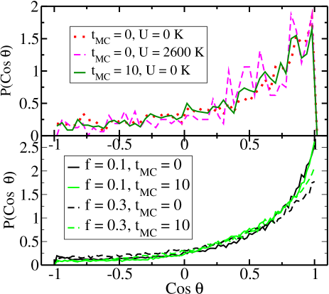
Figure 5: (Color online.) Top: The dependence of the spin distribution function, $P(\cos(\theta))$, on the on-site interaction, $U=U_{N}$, and the Monte Carlo time for $L=10\,a_{\rm lat}$, $x=0.01$, and $f=0.30$. We averaged over 10 samples. Even with interactions and at large Monte Carlo times (small disorder) the spin distribution function remains broad. This is consistent with the strong reduction of the saturation magnetization ($\sim 60\%$) observed in our calculations, independent of Monte Carlo time. Bottom: Dependence of the spin distribution on the hole fraction $f$, $U=0$, obtained after averaging over 100 samples.

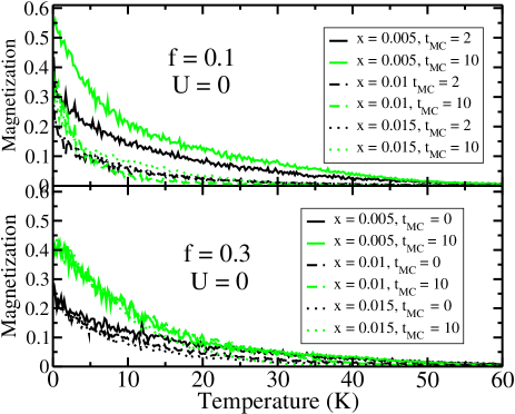
Figure 6: (Color online.) Magnetization as a function of temperature, Mn concentration $x$, and Monte Carlo time $t_{MC}$ for different hole fractions $f$. Here $L=10a_{\rm lat}$, $U=0$, and 100 samples are averaged over. Top: Hole fraction $f=0.1$. Bottom: Hole fraction $f=0.3$. In both cases, as the Monte Carlo time increases, for fixed $x$, the saturation magnetization at zero temperature increases. For both values of $f$ the curves remain linear over a fairly wide temperature range, much the same as for experimentally measured curves for unannealed GaMnAs. The saturation magnetization never reaches more than $\sim 60\%$ of the fully saturated value. This is consistent with the wide spin distribution shown in Fig. 5 and indicates that the ferromagnetism is non-collinear.

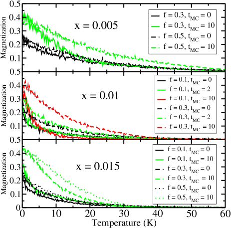
Figure 7: (Color online.) Magnetization as a function of temperature, hole fraction $f$, and Monte Carlo time $t_{MC}$ for different Mn concentrations $x$. Here $L=10\,a_{\rm lat}$, $U=0$ and 100 samples are averaged over. Compare with Fig. 6. Top: Mn concentration $x=0.005$. Middle: Mn concentration $x=0.01$. Bottom: Mn concentration $x=0.015$. The general trend is the same as in Fig. 6: Longer Monte Carlo times lead to larger zero temperature magnetizations. The saturation magnetization is roughly independent of Mn concentration $x$.

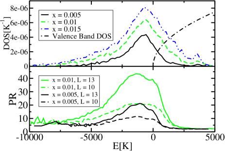
Figure 8: (Color online.) Top: The dependence of the density of states on doping $x$ for $L=10\,a_{\rm lat}$, $f=0.50$, and $t_{MC}=0$. Data is the average of 50 sample realizations. The DOS is normalized to the volume of a unit cell, so the total number of states is proportional to $x$. The half-width of the impurity band ranges from $1000-2500$ K and is centered around -1100 K, the binding energy of a hole at an isolated Mn. The shape of the density of states changes little with the Mn concentration, $x$, over the range of values shown. The value of the Fermi energy is $\approx-5000$ K. For comparison, the valence band density of states is also shown. Bottom: The dependence of the participation ratio on doping $x$. Data is averaged over 50 samples. Larger samples have larger values of the PR for delocalized states, while for localized states the PR is independent of system size for fixed $x$, $t_{MC}=0$. The energy value that separates $L$-dependent PRs from $L$-independent PRs is the mobility edge. This depends on $x$ and is larger for larger $x$. For the disordered samples here, the mobility edge is not too sharp and lies in the tail of the density of states.

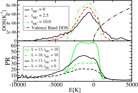
Figure 9: (Color online.) Top: The dependence of the density of states on Monte Carlo time for $U=0$, $x=0.01$, $f=0.30$, and $L=10\,a_{\rm lat}$. Data is the average of 50 sample realizations. MC time $t_{MC}=0$ means that the Mn positions are completely random; for $t_{MC}=10$ the Mn ions form a nearly BCC lattice with a few point defects. The main effect of disorder is thus to broaden the impurity band. The width of the impurity band is proportional to the value of the dominant hopping parameter, $t_{3/2}$, at typical Mn separations as can be seen from Fig. 4. Bottom: The dependence of the PR on the MC time for $x=0.01$ and $f=0.30$. Data is averaged over 50 samples. The mobility edge also moves up to higher energy values for more ordered Mn configurations and nearly all states become delocalized.

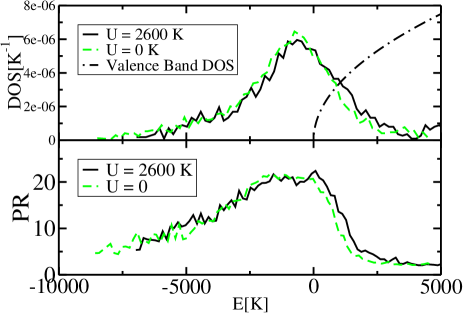
Figure 10: (Color online.) Top: The dependence of the density of states on the on-site interactions, $U=2600$ K, for $x=0.01$, $f=0.30$, and $t_{MC}$. The effect of interactions on the DOS is minimal: The overall shape remains largely unchanged by the interactions. Bottom: The dependence of the PR on the on-site interactions, $U$, for $x=0.01$, $f=0.30$, $L=10\,a_{\rm lat}$, and $t_{MC}=0$. Data is averaged over 10 samples. The behavior of the participation ratio follows roughly that of the density of states shown in Top; There is little shape change compared to the non-interacting case.

IV.2 Results

IV.2.1 Magnetization

Similar to the metallic case within the spherical approximation,Zaránd and Jankó (2002) we find a ferromagnetic state with a largely reduced magnetization, $|\langle\vec{\Omega}_{i}\rangle|\approx 0.4$ for $L=10\,a_{\rm lat}$. (See Figs. 6 and 7.) We find that this reduction is largely due to spin-orbit coupling, and that $\cos(\theta_{i})={\vec{\Omega}_{i}}\cdot{\vec{n}}$, (where ${\vec{n}}$ is the direction of the ground state magnetization vector) has a broad distribution, $P(\cos(\theta))$, quantitatively similar to earlier results obtained in the metallic case using the 4-band spherical approximation in the completely disordered case.Zaránd and Jankó (2002) The interaction Hamiltonian (4) appears to have a negligible effect on the spin distribution. Also, relaxing the Mn impurities to form a regular BCC lattice as described above appears to have little impact on the spin distribution. We checked that this result is valid at least for $f=0.1-0.3$. This is qualitatively different from the metallic case which showed a significant sharpening of the distribution function as the Mn positions became more ordered, and a corresponding increase of the saturation magnetization to an almost fully polarized state.Fiete et al. (2005)

The magnetization for $U=0$ is shown in Figs. 6 and 7. The curves indicate that the system never reaches the fully polarized state, even for long Monte Carlo times. However, as the disorder is reduced the saturation magnetization increases from $\approx 20-25\%$ to $40-50\%$. The magnetization curves exhibit linear behavior over a large temperature range, qualitatively similar to experiments on disordered samples.

Unfortunately, since the numerical calculations are rather demanding, we could not perform a proper finite size scaling analysis. Therefore, while our calculations suggest that the ground state of our model is ferromagnetic, we cannot exclude the possibility of a paramagnetic or spin glass state for these small concentrations.

IV.2.2 Density of States

We compute the DOS from the Hamiltonian (3) and in the interacting case $H_{var}$. The results are shown in Figs. 8-10.

Fig. 8 shows the dependence of the DOS on doping $x$ for fixed MC time and $U_{N}=U_{F}=0$. The total number of states is proportional to $x$. The overall shape is fairly independent of $x$, over the range of $x$ considered here, which shows a peak near the binding energy, $E_{b}\approx-1100$K, of the isolated Mn+hole system and a half-width of 0.1-0.25 eV. The impurity band slightly overlaps the valence band DOS. However, comparison with the valence hole density of states suggests that at concentrations $x\lesssim 0.015$ a well-formed impurity band may still be present, and it might persist to higher concentrations. Indeed, this scenario seems to be supported by many experiments.Singley et al. (2002); Asklund et al. (2002); Singley et al. (2003); Burch et al. (2004); Okabayashi et al. (2001a, b); Grandidier et al. (2000); Tsuruoka et al. (2002)

Fig. 9 shows the dependence of the DOS on MC time for fixed $x$. For $t_{MC}=0$ the Mn ions are completely random while for $t_{MC}=10$ the Mn ions form a nearly perfect BCC lattice with a few point defects. The main effect of disorder, mostly due to the random Coulomb shift of $E_{i}$ in Eq. (26), is to broaden the impurity band DOS. In the ordered case, the width of the impurity band is determined by the value of the dominant hopping parameter, $t_{3/2}$ at the typical Mn separations.

Fig. 10 shows the effects of the interactions on the DOS. Within the variational calculation, the absolute scale of the quasi-particle energies is not given. However, as shown in Fig. 10, the overall shape of the single particle density of states and the energy-dependent participation ratio are almost identical to what we found in our calculations performed for the non-interacting model.

In order to gain information on transport properties of the holes, we turn to an analysis of another quantity, the participation ratio, from which finite size scaling will be able to tell us which states of the impurity band are localized and which states are delocalized in the impurity band.

IV.2.3 Participation Ratios

The participation ratio, ${\rm PR}=[\sum_{i}(\sum_{\alpha}|\psi_{i\alpha}|^{2})^{2}]^{-1}$, measures the degree to which wavefunctions are localized. If states are completely delocalized, the single particle wavefunction $\psi_{i\alpha}$ will be spread equally over all sites making the PR system-size dependent because the wavefunction must be normalized to unity. Thus, the PR grows with system size for delocalized states while the it remains ${\cal O}$(1) in the thermodynamic limit for localized states.

Fig. 8 shows the dependence of the PR on $x$ and system size $L$ for fixed disorder. Larger samples have larger values of the PR for delocalized states while for localized states the PR is $L$ independent. The energy joining the two regimes is the mobility edge. It is impossible to determine the precise position of the mobility edge from our numerics, but in both cases, the Fermi energy apparently lies in the region of delocalized states, indicating a localization transition in the impurity band itself.

Fig. 9 shows the dependence of the PR on disorder. For small disorder, nearly all states become delocalized and similar to the the disordered case the localization transition occurs in the impurity band.

Fig. 10 shows the dependence of the PR on the on-site interactions in Eq. (4). The behavior of the PR ratio roughly follows that of the DOS shown in Fig. 10: There is little shape change with the interactions, and the result looks very similar to the non-interacting case. Thus, the relation between the mobility edge and the Fermi energy remains essentially unchanged implying that the localization transition is robust to reasonable on-site interactions.

To summarize the result of this section, we find that the chemical potential lies deep ($\sim 0.5-0.7\,{\rm eV}$) inside the gap. From the PR data, it appears that the chemical potential is in the vicinity of the mobility edge, a regime where our model is probably more reliable. This suggests that the localization phase transition in ${\rm Ga}_{1-x}{\rm Mn}_{x}{\rm As}$ could happen inside the impurity band and that the ferromagnetic phase for smaller Mn concentrations is governed by localized hole states. Fiete et al. (2003); Berciu and Bhatt (2001, 2004); Timm et al. (2002); Yang and MacDonald (2003); Chattopadhyay et al. (2001); Galitski et al. (2004)

V Conclusions

Starting with a single Mn acceptor state in GaMnAs, we derived an effective Hamiltonian for ${\rm Ga}_{1-x}{\rm Mn}_{x}{\rm As}$ valid in the dilute limit, where ${\rm Ga}_{1-x}{\rm Mn}_{x}{\rm As}$ can be described in terms of spin $F=3/2$ polarons hopping between the Mn sites and coupled to the local Mn spins. We estimated the parameters of this model from microscopic calculations using both a variational approach and an exact diagonalization for a pair of Mn ions within the spherical approximation. Our approach treats the extremely large Coulomb interaction in a non-perturbative way, and captures the effects of strong spin-orbit coupling, and disorder. We find that due to the large spin-orbit coupling of GaAs, the hopping matrix elements of the polarons depend on their spin direction.

We studied the above effective Hamiltonianon using mean field and variational methods, also including the effects of interactions between the holes. We find that the spin-dependent hopping generates frustration and is ultimately responsible for the formation of a non-collinear magnetic state for small active Mn concentrations. The existence of such non-collinear ground states is indeed supported by experiments, where a substantial increase in the remanent magnetization is found upon the application of a relatively small magnetic field in some unannealed samples.Ku et al. (2003)

Our calculations also support the existence of an impurity band, and a metal-insulator phase transition inside this impurity band for these small concentrations of active Mn ions, in agreement with angle resolved photoemission (ARPES) data,Asklund et al. (2002); Okabayashi et al. (2001a, b) scanning tunneling microscope (STM) results,Grandidier et al. (2000); Tsuruoka et al. (2002) and optical conductivity measurements.Singley et al. (2002, 2003)

The main advantage of our approach is that it provides a clear description of the most important physical ingredients needed to describe dilute ${\rm Ga}_{1-x}{\rm Mn}_{x}{\rm As}$, while it treats the extremely large Coulomb potential of charged substitutional Mn ions non-perturbatively. While the resulting effective Hamiltonian given by Eqs. (3) and (4) is relatively simple, it captures many of the physical properties of ${\rm Ga}_{1-x}{\rm Mn}_{x}{\rm As}$, and can serve as a starting point for field theoretical computations of other physical quantities of interest such as optical conductivity, spin wave relaxation rate, conductivity or (anomalous) Hall resistance.

Though the parameters of our effective Hamiltonian have been determined from microscopic model calculations, they are only approximate: while the spherical approximation used is able to reproduce the spectrum of a single acceptor rather well, it certainly overestimates the effect of spin-orbit coupling and the width of the impurity band. A direct comparison of the parameters in Fig. 4 with those obtained from a more accurate six-band model calculation shows some important quantitative differences.Redlinski et al. (2005) This comparison reveals that while for $r\gtrsim 13\AA$ the effective Hamiltonian (3) is indeed a good approximation in form, the hopping parameters are smaller by a factor of two compared to the ones obtained from the six band model variational calculation. Moreover, for $r\lesssim 13\AA$, the six-band model gives $t_{3/2}\approx t_{1/2}$, suggesting that spin anisotropy is much smaller than that obtained from the spherical model. Furthermore, for shorter Mn separations the effective model turns out to be a rather poor approximation.Redlinski et al. (2005)

In summary, based on microscopic calculations, we constructed a many-body Hamiltonian that is appropriate for describing ${\rm Ga}_{1-x}{\rm Mn}_{x}{\rm As}$ in the very dilute limit, and estimated its parameters. We find that the hopping of the carriers is strongly correlated with their spin. This spin-dependent hopping is crucial for capturing spin-orbit coupling induced random anisotropy terms, or the lifetime of the magnon excitations. Our calculations support the presence of an impurity band for $x_{\rm active}\lesssim 0.015$ active Mn concentration.

Appendix A Expressions for Angular Dependence of Induced Hole Polarization

With the wavefunctions (7) in hand, we can calculate the average hole spin density around an isolated Mn impurity, $\langle\vec{j}(r,\theta,\phi)\rangle$, which reflects the partial $d$-wave character of the Baldereschi-Lipari wavefunctions. As an example, consider $\langle j_{z}(r,\theta,\phi)\rangle_{F_{z}=3/2}$. Using the angular momentum addition rules we can express the orbital parts of the wave functions in Eq. (7) as

$$|L=0,j=\frac{3}{2},F=\frac{3}{2},F_{z}=\frac{3}{2}\rangle\to Y_{0}^{0}\;|\frac{3}{2}\rangle,$$ (30)

$$|L=2,j=\frac{3}{2},F=\frac{3}{2},F_{z}=\frac{3}{2}\rangle\to$$ (31)

$$\phantom{nn}\to\sqrt{{2\over 5}}\;Y_{2}^{2}\;|-\frac{1}{2}\rangle-\sqrt{{2\over 5}}\;Y_{2}^{1}\;|\frac{1}{2}\rangle+\sqrt{{1\over 5}}\;Y_{2}^{0}\;|\frac{3}{2}\rangle\;,$$

where the $Y_{l}^{m}$ denote the spherical functions, and the second terms stand for the spin part of the $j=3/2$ wave function. Thus the full wave function reads

$$\Phi_{F_{z}=3/2}=\left(f_{0}(r)Y_{0}^{0}(\theta,\phi)+{g_{0}(r)\over\sqrt{5}}Y_{2}^{0}(\theta,\phi)\right)\Bigl{|}\frac{3}{2}\Bigr{\rangle}$$

$$\phantom{nn}-g_{0}(r)\sqrt{{2\over 5}}Y_{2}^{1}(\theta,\phi)\Bigl{|}\frac{1}{2}\Bigr{\rangle}+g_{0}(r)\sqrt{{2\over 5}}Y_{2}^{2}(\theta,\phi)\Bigl{|}-\frac{1}{2}\Bigr{\rangle}\;.$$

Taking the expectation value of $j_{\|}\equiv j_{z}$ in this state gives, along with analogous calculations in the other states and for the perpendicular component of the spin, $j_{\perp}\equiv\cos(\phi)\;j_{x}+\sin(\phi)\;j_{y}$,

$$\langle j_{\|}(\vec{r})\rangle_{F_{z}=\pm 3/2} = \pm{3\over 8\pi}\left[f_{0}(r)^{2}+f_{0}(r)g_{0}(r)(3{\rm cos}^{2}(\theta)-1)+g_{0}(r)^{2}{\rm cos}^{4}(\theta)\right]\;,$$ (33)

$$\langle j_{\bot}(\vec{r})\rangle_{F_{z}=\pm 3/2} = \pm{3\over 4\pi}\left[(f_{0}(r)+{g_{0}(r)\over 2}(3{\rm cos}^{2}(\theta)-1))g_{0}(r)+g_{0}(r)^{2}{\rm sin}^{2}(\theta)\right]{\rm sin}(\theta){\rm cos}(\theta)\;,$$ (34)

$$\langle j_{\|}(\vec{r})\rangle_{F_{z}=\pm 1/2} = \pm{1\over 8\pi}\Biggl{[}f_{0}(r)^{2}-f_{0}(r)g_{0}(r)(3{\rm cos}^{2}(\theta)-1)+{g_{0}(r)^{2}\over 8}(5+12{\rm cos}(2\theta)-9{\rm cos}(4\theta))\Biggr{]}\;,$$ (35)

$$\langle j_{\bot}(\vec{r})\rangle_{F_{z}=\pm 1/2} = \pm{3\over 4\pi}\Biggl{[}(f_{0}(r)-{g_{0}(r)\over 2}(3{\rm cos}^{2}(\theta)-1))g_{0}(r)\Biggr{]}{\rm sin}(\theta){\rm cos}(\theta)\;.$$ (36)

Appendix B Two-ion Problem

Here we derive the parameters of the effective Hamiltonian (15) using the molecular orbitals for a pair of Mn ions.Durst et al. (2002) Since the exchange interaction with the Mn core is much less than the binding energy of the holes, and the on-site interaction energy, we neglect its effect on the parameters of the effective Hamiltonian (15). The local field created by the Mn core spin on the holes is later treated self-consistently in a mean field and variational calculation described in Sec. IV.

We solve the problem in the eight-dimensional subspace spanned by the $F=3/2$ acceptor states centered on each impurity obtained through the variational calculations of Sec. II. As we discussed in the main text, within the spherical approximation used throughout this paper, $F_{z}$ is conserved if the two impurities are aligned along the $z$ axis. In this case the sectors of different $F_{z}$ decouple. Furthermore, because of time reversal symmetry, the overlap matrices $S$ (see Sec. II) and Hamiltonian matrix elements are identical for $F_{z}=\pm 3/2$ and for $F_{z}=\pm 1/2$. In the $F_{z}=\pm 3/2$ sector these are given by

$$S^{(3/2)}=\pmatrix{1&a_{+}\cr a_{+}&1\cr}$$ (37)

and

$$H^{(3/2)}=\pmatrix{E_{0}+e_{1}&e_{3}+a_{+}\;E_{0}\cr e_{3}+a_{+}\;E_{0}&E_{0}+e_{1}\cr}\;,$$ (38)

while for the $F_{z}=\pm 1/2$ subspace we have

$$S^{(1/2)} = \pmatrix{1&a_{-}\cr a_{-}&1\cr}\;$$ (39)

$$H^{(1/2)} = \pmatrix{E_{0}+e_{2}&e_{4}+a_{-}\;E_{0}\cr e_{4}+a_{-}\;E_{0}&E_{0}+e_{2}\cr}\;.$$ (40)

The two columns of these matrices correspond to the two Mn sites, and the constants $a_{\pm}$, and $e_{1},\dots e_{4}$ denote various matrix elements between the wavefunction of a hole at site 1 and a hole at site 2. The explicit formulas for these quantities are given below. $E_{0}$ is the ground state energy of the single bound hole as determined in Sec. II. Using Eq. (7), expanding the angular parts in spherical harmonics and then rewriting the expressions in cylindrical coordinates, we have $r=\sqrt{\rho^{2}+z^{2}}$, with $\rho$ the radial coordinate. To simplify our expressions, we introduce the notations $f_{0}\equiv f_{0}(r(\rho,z))$ (likewise for $g_{0}$), $\tilde{z}\equiv z-z_{0}$, $\tilde{r}\equiv\sqrt{\rho^{2}+(z-z_{0})^{2}}$, and ${\tilde{f}}_{0}=f_{0}(\tilde{r})$ (and likewise for ${\tilde{g}}_{0}\equiv g_{0}(\tilde{r})$), with $z_{0}$ the distance between the two impurities, and express the above matrix elements as

$$a_{\pm} = \int_{0}^{\infty}\rho d\rho\int_{-\infty}^{\infty}dz\Biggl{[}{1\over 2}\left(f_{0}\pm{g_{0}\over 2}\left(3{z^{2}\over r^{2}}-1\right)\right)\left({\tilde{f}}_{0}\pm{{\tilde{g}}_{0}\over 2}\left(3{{\tilde{z}}_{0}^{2}\over{\tilde{r}}^{2}}-1\right)\right)+{3\over 2}\;g_{0}\;{\tilde{g}}_{0}\;{\rho^{2}\over r^{2}{\tilde{r}}^{2}}\left(z\tilde{z}+{1\over 4}\rho^{2}\right)\Biggr{]}\;,$$ (41)

$$e_{1,2} = \int_{0}^{\infty}\rho d\rho\int_{-\infty}^{\infty}dz\;V_{2}(\tilde{r})\;\Biggl{[}{1\over 2}\left(f_{0}\pm{g_{0}\over 2}\left(3{z^{2}\over r^{2}}-1\right)\right)^{2}+{3\over 2}g_{0}^{2}{\rho^{2}\over r^{4}}\left(z^{2}+{1\over 4}\rho^{2}\right)\Biggr{]}\;,$$ (42)

$$e_{3,4} = \int_{0}^{\infty}\rho d\rho\int_{-\infty}^{\infty}dz\;V_{2}(\tilde{r})\;\Biggl{[}{1\over 2}\left(f_{0}\pm{g_{0}\over 2}\left(3{z^{2}\over r^{2}}-1\right)\right)\left({\tilde{f}}_{0}\pm{{\tilde{g}}_{0}\over 2}\left(3{{\tilde{z}}_{0}^{2}\over{\tilde{r}}^{2}}-1\right)\right)+{3\over 2}\;g_{0}\;{\tilde{g}}_{0}\;{\rho^{2}\over r^{2}{\tilde{r}}^{2}}\left(z\tilde{z}+{1\over 4}\rho^{2}\right)\Biggr{]},$$ (43)

where $V_{2}\equiv V_{1}(\tilde{r})$ is given by Eq. (14). It should be kept in mind that $a_{\pm}$, the hole binding energy $E_{0}$ and the four $e_{i}$ all depend on the spherical spin-orbit strength $\mu$, and must be evaluated numerically. These parameters are shown in Figs. 11 and 12. Having these parameters at hand, we can simply determine the effective parameters $t_{1/2}$, $t_{3/2}$, $K$, and $E$ in Eq. (15) by equating the spectrum of the two Mn ions with that of the effective Hamiltonian Eq. (15). In this way we obtain

$$t_{3/2} = \frac{a_{+}e_{1}-e_{3}}{a_{+}^{2}-1}\;,$$ (44)

$$t_{1/2} = \frac{a_{-}e_{2}-e_{4}}{a_{-}^{2}-1}\;,$$ (45)

$$K = \frac{1}{2}\left({a_{+}e_{3}-e_{1}\over a_{+}^{2}-1}-{a_{-}e_{4}-e_{2}\over a_{-}^{2}-1}\right)\;,$$ (46)

$$E = \frac{1}{2}\left({a_{+}e_{3}-e_{1}\over a_{+}^{2}-1}+{a_{-}e_{4}-e_{2}\over a_{-}^{2}-1}\right)\;.$$ (47)

These parameters have been plotted in Fig. 4.

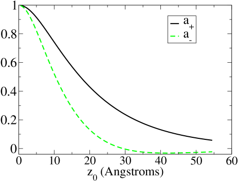
Figure 11: (Color online.) Wave function overlaps for the two states on site 1 and site 2. The overlaps are computed from Eq. (B5).

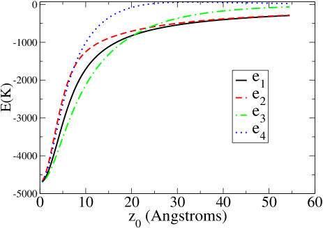
Figure 12: (Color online.) Interaction overlaps for the interactions defined in the text, Eqs. (B6) and (B7).

Appendix C Derivation and Evaluation of On-site Interactions $U_{N}$ and $U_{F}$

In the dilute limit it is important to include the effects of interactions between holes. Here we only consider the on-site interaction of the holes which dominate all other interactions due to the localized nature of the molecular orbitals.

In second quantized form the interaction between two holes is

$$\hat{H}_{\rm on-site}=\frac{1}{2}\sum_{f_{1},f_{2},f_{3},f_{4}}U_{f_{1},f_{2},f_{3},f_{4}}c^{\dagger}_{f_{1}}c^{\dagger}_{f_{2}}c_{f_{3}}c_{f_{4}}\;,$$ (48)

where $U_{f_{1},f_{2},f_{3},f_{4}}$ denotes the usual Coulomb integral

$$U_{f_{1},f_{2},f_{3},f_{4}}=\sum_{\mu,\nu}\int d^{3}\vec{r}\int d^{3}\vec{r}^{\prime}\Phi^{*}_{f_{1}}(\vec{r},\mu)\Phi_{f_{4}}(\vec{r},\mu)$$

$$\times{e^{2}\over\epsilon|\vec{r}-\vec{r}^{\prime}|}\Phi^{*}_{f_{2}}(\vec{r}^{\prime},\nu)\Phi_{f_{3}}(\vec{r}^{\prime},\nu)\;,$$ (49)

and where we have again restricted ourselves to the same $F=3/2$ subspace, and correspondingly the eigenvalues of the z-component of $F_{z}$, $f_{i}$, may take on the values $\pm 3/2$ and $\pm 1/2$. Here $\mu,\nu$ are the eigenvalues of $j_{z}$. The wave functions $\Phi_{f_{i}}(\vec{r},\mu)$ have been determined previously with the variational calculation outlined in Sec II. (See Eq. (7) and Eq. (A) for an illustration of how the angular dependence of $\Phi_{f_{i}}(\vec{r},\mu)$ is obtained. A simple projection of $\langle j=3/2,j_{z}=\mu=1/2|$ into Eq. (A) picks out $\Phi_{3/2}(\vec{r},1/2)=-g_{0}(r)\sqrt{{2\over 5}}Y_{2}^{1}(\theta,\phi)$, for example.)

Fortunately, we do not have to compute all these matrix elements if we rewrite Eq. (48) in terms of two-hole scattering processes and exploit rotational symmetry. Two holes can only take an $F=0$ or an $F=2$ configuration within the ground state multiplet because of the Pauli principle. One can verify by direct evaluation that the $F=F_{z}=2$ two-hole state is created by the following operator from the vacuum,

$$\hat{D}_{2}=c^{\dagger}_{1/2}\;c^{\dagger}_{3/2}\;,$$ (50)

while the $F=2$ states of lower $F_{z}$ can be produced by applying the lowering operator. The corresponding operators read:

$$\hat{D}_{1} = c^{\dagger}_{-1/2}\;c^{\dagger}_{3/2}\;,$$ (51)

$$\hat{D}_{0} = \frac{1}{\sqrt{2}}(c^{\dagger}_{-3/2}\;c^{\dagger}_{3/2}+c^{\dagger}_{-1/2}\;c^{\dagger}_{1/2})\;,$$ (52)

$$\hat{D}_{-1} = c^{\dagger}_{-3/2}\;c^{\dagger}_{1/2}\;,$$ (53)

$$\hat{D}_{-2} = c^{\dagger}_{-3/2}\;c^{\dagger}_{-1/2}\;.$$ (54)

Likewise for the sole $F=0$ operator we get,

$$\hat{S}_{0}=\frac{1}{\sqrt{2}}(c^{\dagger}_{-1/2}\;c^{\dagger}_{1/2}-c^{\dagger}_{-3/2}\;c^{\dagger}_{3/2})\;.$$ (55)

Since these operators transform as $F=0$ and $F=2$ tensor operators under SU(2) rotations, the interaction Hamiltonian must have the form

$$\hat{H}_{\rm on-site}=U_{D}\sum_{m}\hat{D}^{\dagger}_{m}\hat{D}_{m}+U_{S}\hat{S}^{\dagger}_{0}\hat{S}_{0}\;.$$ (56)

We can, however, use instead of the decomposition above the following two SU(2) invariants too:

$$\hat{H}_{\rm int}=\frac{U_{N}}{2}:{\hat{N}}^{2}:+\,\frac{U_{F}}{2}:\vec{F}^{2}:\;,$$ (57)

where $:\dots:$ denotes normal ordering and $\hat{N}=\sum_{f}c^{\dagger}_{f}c_{f}$, and $\hat{\vec{F}}=\sum_{f,f^{\prime}}c^{\dagger}_{f}\vec{F}_{f,f^{\prime}}c_{f^{\prime}}$ denote the number of holes and their total spin operator. It is easy to determine the relation of the constants $U_{F}$ and $U_{N}$ to $U_{D}$ and $U_{S}$ if one rewrites Eq. (57) using the identities

$$:{\hat{N}}^{2}: = {\hat{N}}^{2}-{\hat{N}}\;,$$

$$:\vec{F}^{2}: = \vec{F}^{2}-\frac{15}{4}{\hat{N}}\;,$$ (58)

and compares the action of Eq. (56) and Eq. (57) on the $N=2$ and $F=0,2$ states. This simple algebra gives:

$$U_{N} = \frac{5U_{D}-U_{S}}{4}\;,$$ (59)

$$U_{F} = \frac{U_{D}-U_{S}}{3}\;.$$ (60)

By comparing the matrix elements of Eq. (56) to the matrix elements of Eq. (48), we can evaluate $U_{D}$ and $U_{S}$ in terms of the $U_{f_{1},f_{2};f_{4},f_{3}}\equiv U_{f_{1},f_{2},f_{3},f_{4}}$ which in turn allow us to evaluate the $U_{N}$ and $U_{F}$ of Eq. (57). Carrying out this calculation, one obtains

$$U_{D} = 2\left(U_{\frac{3}{2},\frac{1}{2};\frac{3}{2},\frac{1}{2}}-U_{\frac{3}{2},\frac{1}{2};\frac{1}{2},\frac{3}{2}}\right)$$ (61)

$$U_{S} = 4\left(U_{\frac{1}{2},-\frac{1}{2};\frac{1}{2},-\frac{1}{2}}-U_{\frac{1}{2},-\frac{1}{2};-\frac{1}{2},\frac{1}{2}}\right)-U_{D}\;,$$

and therefore,

$$U_{N} = 3\left(U_{\frac{3}{2},\frac{1}{2};\frac{3}{2},\frac{1}{2}}-U_{\frac{3}{2},\frac{1}{2};\frac{1}{2},\frac{3}{2}}\right)$$ (63)

$$- U_{\frac{1}{2},-\frac{1}{2};\frac{1}{2},-\frac{1}{2}}+U_{\frac{1}{2},-\frac{1}{2};-\frac{1}{2},\frac{1}{2}}$$

$$U_{F} = \frac{4}{3}\Bigl{(}U_{\frac{3}{2},\frac{1}{2};\frac{3}{2},\frac{1}{2}}-U_{\frac{3}{2},\frac{1}{2};\frac{1}{2},\frac{3}{2}}$$ (64)

$$- U_{\frac{1}{2},-\frac{1}{2};\frac{1}{2},-\frac{1}{2}}+U_{\frac{1}{2},-\frac{1}{2};-\frac{1}{2},\frac{1}{2}}\Bigr{)}\;.$$

To obtain a numerical value of $U_{N}$ and $U_{F}$ we must determine the matrix elements $U_{3/2,1/2;3/2,1/2}$, $U_{3/2,1/2;1/2,3/2}$, $U_{1/2,-1/2;1/2,-1/2}$ and $U_{1/2,-1/2;-1/2,1/2}$ by evaluating the integrals in Eq. (49). These integrals depend on the radial wave functions that we evaluated variationally in Sec. II and are material (parameter) specific. In order to evaluate the integrals in Eq. (49) the $\Phi_{\mu,f_{i}}(\vec{r})$ must be decomposed into spherical harmonics. Various products of spherical harmonics appear in the integrand. The integrals can be evaluated by making use of the important formula

$${1\over|\vec{r}-\vec{r}^{\prime}|}=\frac{4\pi}{r_{>}}\sum_{l=0}^{\infty}\sum_{m=-l}^{l}\left(\frac{r_{<}}{r_{>}}\right)^{l}\frac{(-1)^{m}}{2l+1}{Y_{l}^{m}}^{*}(\Omega)Y_{l}^{m}(\Omega^{\prime})\;,$$ (65)

where $\Omega$ ($\Omega^{\prime}$) is the angle of $\vec{r}$ ($\vec{r}^{\prime}$). Here $r_{>}$ ($r_{<}$) is the greater (lesser) of $r$ and $r^{\prime}$. With this formula, most of the integrals vanish and the few remaining integrals yield

$$U_{\frac{3}{2},\frac{1}{2};\frac{3}{2},\frac{1}{2}} = \frac{e^{2}}{\epsilon a_{\rm eff}}\;(I_{1}-I_{2})\;,$$ (66)

$$U_{\frac{3}{2},\frac{1}{2};\frac{1}{2},\frac{3}{2}} = \frac{e^{2}}{\epsilon a_{\rm eff}}\;2I_{2}\;,$$ (67)

$$U_{\frac{1}{2},-\frac{1}{2};\frac{1}{2},-\frac{1}{2}} = \frac{e^{2}}{\epsilon a_{\rm eff}}\;(I_{1}+I_{2})\;,$$ (68)

$$U_{\frac{1}{2},-\frac{1}{2};-\frac{1}{2},\frac{1}{2}} = 0\;,$$ (69)

where the prefactor gives the energy scale of the interaction,

$$\frac{e^{2}}{\epsilon a_{\rm eff}}=31.6\;{\rm meV}\;,$$ (70)

and $I_{1}$ and $I_{2}$ denote the following integrals:

$$I_{1} = \int_{0}^{\infty}\!\!\!r^{2}dr\int_{0}^{\infty}\!\!\!r^{\prime 2}dr^{\prime}\frac{1}{r_{>}}(f^{2}_{0}(r)+g^{2}_{0}(r))$$ (71)

$$\phantom{nnn}\times(f^{2}_{0}(r^{\prime})+g^{2}_{0}(r^{\prime}))\;,$$

$$I_{2} = \int_{0}^{\infty}\!\!\!r^{2}dr\int_{0}^{\infty}\!\!\!r^{\prime 2}dr^{\prime}\frac{4}{25}\frac{r_{<}^{2}}{r_{>}^{3}}f_{0}(r)g_{0}(r)f_{0}(r^{\prime})g_{0}(r^{\prime})\;.$$

Evaluating these integrals one obtains $U_{N}=2570\;{\rm K}$ and $U_{F}=-51\;{\rm K}$.

References

- (1) For reviews see A. H. MacDonald, P. Schiffer, and N. Samarth, Nature Materials, 4, 195 (2005); J. König et al. in Electronic Structure and Magnetism of Complex Materials, edited by D.J. Singh and D.A. Papaconstantopoulos (Springer Verlag 2002); R. N. Bhatt et al., J. Superconductivity INM 15, 71 (2002); F. Matsukura and H. Ohno and T. Dietl in:Handbook on Magnetic Materials, Elsevier 2002.
- DiVincenzo (1995) D. P. DiVincenzo, Science 270, 255 (1995).
- Nielson and Chuang (2000) M. A. Nielson and I. L. Chuang, Quantum Computation and Quantum Information (Cambridge University Press, Cambridge, UK, 2000).
- Awschalom et al. (2002) D. D. Awschalom, N. Samarth, and D. Loss, eds., Semiconductor Spintronics and Quantum Computation (Springer Verlag, Heidelberg, 2002).
- Zutic et al. (2004) I. Zutic, J. Fabian, and S. D. Sarma, Rev. Mod. Phys. 76, 323 (2004).
- Ohno (1998) H. Ohno, Science 281, 951 (1998).
- Edmonds et al. (2004) K. W. Edmonds, P. Boguslawski, K. Y. Wang, R. P. Campion, N. R. S. Farley, B. Gallagher, C. T. Foxon, M. Sawicki, T. Dietl, M. B. Nardelli, et al., Phys. Rev. Lett. 92, 037201 (2004).
- Linnarsson et al. (1997) M. Linnarsson, E. Janzén, B. Monemar, M. Kleverman, and A. Thilderkvist, Phys. Rev. B 55, 6938 (1997).
- Singley et al. (2002) E. J. Singley, R. Kawakami, D. D. Awschalom, and D. N. Basov, Phys. Rev. Lett. 89, 097203 (2002).
- Singley et al. (2003) E. J. Singley, K. S. Burch, R. Kawakami, J. Stephens, D. D. Awschalom, and D. N. Basov, Phys. Rev. B 68, 165204 (2003).
- Burch et al. (2004) K. S. Burch, J. Stephens, R. K. Kawakami, D. D. Awschalom, and D. N. Basov, Phys. Rev. B 70, 205208 (2004).
- Asklund et al. (2002) H. Asklund, L. Ilver, J. Kanski, J. Sadowski, and R. Mathieu, Phys. Rev. B 66, 115319 (2002).
- Okabayashi et al. (2001a) J. Okabayashi, A. Kimura, O. Rader, T. Mizokawa, A. Fujimori, T. Hayashi, and M. Tanaka, Phys. Rev. B 64, 125304 (2001a).
- Okabayashi et al. (2001b) J. Okabayashi, A. Kimura, O. Rader, T. Mizokawa, A. Fujimori, T. Hayashi, and M. Tanaka, Physica E 10, 192 (2001b).
- Grandidier et al. (2000) B. Grandidier, J. P. Nys, C. Delerue, D. Stiévenard, Y. Higo, and M. Tanaka, Appl. Phys. Lett. 77, 4001 (2000).
- Tsuruoka et al. (2002) T. Tsuruoka, N. Tachikawa, S. Ushioda, F. Matsukura, K. Takamura, and H. Ohno, Appl. Phys. Lett. 81, 2800 (2002).
- Esch et al. (1997) A. V. Esch, L. V. Bockstal, J. D. Boeck, G. Verbanck, A. S. van Steenbergen, and P. J. Wellmann, Phys. Rev. B 56, 13103 (1997).
- Kennett et al. (2002a) M. P. Kennett, M. Berciu, and R. N. Bhatt, Phys. Rev. B 66, 045207 (2002a).
- Fiete et al. (2003) G. A. Fiete, G. Zaránd, and K. Damle, Phys. Rev. Lett. 91, 097202 (2003).
- Berciu and Bhatt (2001) M. Berciu and R. N. Bhatt, Phys. Rev. Lett. 87, 107203 (2001).
- Zhou et al. (2004) C. Zhou, M. P. Kennett, X. Wan, M. Berciu, and R. N. Bhatt, Phys. Rev. B 69, 144419 (2004).
- Hankiewicz et al. (2004) E. M. Hankiewicz, T. Jungwirth, T. Dietl, C. Timm, and J. Sinova, Phys. Rev. B 70, 245211 (2004).
- Timm et al. (2002) C. Timm, F. Schäfer, and F. von Oppen, Phys. Rev. Lett. 89, 137201 (2002).
- Mahadevan and Zunger (2004) P. Mahadevan and A. Zunger, Phys. Rev. B 69, 115211 (2004).
- Averkiev and ll’inski (1994) N. S. Averkiev and S. Y. ll’inski, Phys. Solid State 36(2), 278 (1994).
- Baldereschi and Lipari (1973) A. Baldereschi and N. O. Lipari, Phys. Rev. B 62, 2697 (1973).
- Tang and Flatté (2004) J.-M. Tang and M. E. Flatté, Phys. Rev. Lett. 92, 047201 (2004).
- Yakunin et al. (2004) A. M. Yakunin, A. Y. Silov, P. M. Koenraad, J. H. Wolter, W. V. Roy, J. DeBoeck, J.-M. Tang, and M. E. Flatté, Phys. Rev. Lett. 92, 216806 (2004).
- Zaránd and Jankó (2002) G. Zaránd and B. Jankó, Phys. Rev. Lett. 89, 047201 (2002).
- Fiete et al. (2005) G. A. Fiete, G. Zaránd, B. Jankó, P. Redliński, and C. P. Moca, Phys. Rev. B 71, 115202 (2005).
- Redlinski et al. (2005) P. Redliński, G. Zaránd, B. Jankó, (unpublished).
- Bergqvist et al. (2003) L. Bergqvist, P. A. Korzhavyi, B. Sanyal, S. Mirbt, I. A. Abrikosov, L. Nordström, E. A. Smirnova, P. Mohn, P. Svedlindh, and O. Eriksson, Phys. Rev. B 67, 205201 (2003).
- Yu et al. (2002a) K. M. Yu, W. Walukiewicz, T. Wojtowicz, I. Kuryliszn, X. Liu, S. Sasaki, and J. K. Furdyna, Phys. Rev. B 65, 201303 (2002a).
- Potashnik et al. (2001) S. J. Potashnik, K. C. Ku, S. H. Chun, J. J. Berry, N. Samarth, and P. Schiffer, Appl. Phys. Lett. 79, 1495 (2001).
- Ku et al. (2003) K. C. Ku, S. J. Potashnik, R. F. Wang, S. H. Chun, P. Schiffer, N. Samarth, M. J. Seong, A. Mascarenhas, E. Johnston-Halperin, R. C. Meyers, et al., Appl. Phys. Lett. 82, 2302 (2003).
- Yu et al. (2002b) K. M. Yu, W. Walukiewicz, T. Wojtowicz, W. L. Lim, X. Liu, Y. Sasaki, M. Dobrowolska, and J. K. Furdyna, Appl. Phys. Lett. 81, 844 (2002b).
- Hayashi et al. (2001) T. Hayashi, Y. Hashimoto, S. Katsumoto, and Y. Iye, Appl. Phys. Lett. 78, 1691 (2001).
- Tim (a) For a recent topical review on defects in GaMnAs see: C. Timm, J. Phys. Cond. Matt. 15, R1865 (2003).
- Bhattacharjee and á la Guillaume (2000) A. K. Bhattacharjee and C. B. á la Guillaume, Solid State Comm. 113, 17 (2000).
- Yang and MacDonald (2003) S.-R. Yang and A. H. MacDonald, Phys. Rev. B 67, 155202 (2003).
- Durst et al. (2002) A. C. Durst, R. N. Bhatt, and P. A. Wolff, Phys. Rev. B 65, 235205 (2002).
- Kennett et al. (2002b) M. P. Kennett, M. Berciu, and R. N. Bhatt, Phys. Rev. B 66, 045207 (2002b).
- Xu et al. (2005) J. L. Xu, M. van Shilfgaarde, and G. D. Samolyuk, Phys. Rev. Lett. 94, 097201 (2005).
- Tim (b) C. Timm and A. H. MacDonald, cond-mat/0405484.
- Chattopadhyay et al. (2001) A. Chattopadhyay, S. D. Sarma, and A. J. Millis, Phys. Rev. Lett. 87, 227202 (2001).
- Berciu and Bhatt (2004) M. Berciu and R. N. Bhatt, Phys. Rev. B 69, 045202 (2004).
- Galitski et al. (2004) V. M. Galitski, A. Kaminski, and S. D. Sarma, Phys. Rev. Lett. 92, 177203 (2004).