Scaling Relations in the Triplet Superconductor PrOs₄Sb₁₂

Abstract

Scaling relations are one of the hallmarks of nodal superconductivity since they contain information characteristic for gapless order parameters. In this paper we derive the scaling relations for the thermodynamics and the thermal conductivity in the vortex state of the A and B phases of the skutterudite PrOs₄Sb₁₂. Experimental verification of these scaling relations can provide further support for anisotropic gap functions which were previously considered for this material.

1. Introduction

Superconductivity in the filled skutterudite PrOs₄Sb₁₂ was discovered in 2002 by Bauer et al 1 ; 2 ; 3 , and has since generated ever-increasing attention. In particular, the presence of at least two distinct phases, the A and B phase, in an applied magnetic field is of great interest. Experimentally, it was observed that both phases have point nodes, and that the pairing channel appears to be a triplet with chiral symmetry breaking. 4 ; 5 ; 6 . However, the precise position of the A-B phase boundary is still controversial. For example, Measson et al 7 found the A-B phase boundary to be almost parallel to H${}_{c2}(T)$ of the A phase. A possible explanation of this phase diagram was recently proposed in terms of the gap functions 6 ; 8

$${\bf\Delta}_{A}({\bf k}) = {\bf d}e^{\pm i\phi_{i}}\frac{3}{2}(1-\hat{k}_{x}^{4}-\hat{k}_{y}^{4}-\hat{k}_{z}^{4}),$$ (1)

$${\bf\Delta}_{B}({\bf k}) = {\bf d}e^{\pm i\phi_{3}}(1-\hat{k}_{z}^{4}).$$ (2)

Here $e^{\pm i\phi_{1}}=(\hat{k}_{2}\pm i\hat{k}_{3})/\sqrt{\hat{k}_{2}^{2}+\hat{k}_{3}^{2}},e^{\pm i\phi_{2}}=(\hat{k}_{3}\pm i\hat{k}_{1})/\sqrt{\hat{k}_{3}^{2}+\hat{k}_{1}^{2}}$, and $e^{\pm i\phi_{3}}=(\hat{k}_{1}\pm i\hat{k}_{2})/\sqrt{\hat{k}_{1}^{2}+\hat{k}_{2}^{2}}$. The factor of 3/2 in the definition of ${\bf\Delta}_{A}({\bf k})$ ensures proper normalization of the angular dependence of the order parameter. Furthermore, in Eq.(2) we choose the nodal direction to be parallel to [001], because this p+h-wave order parameter symmetry is consistent with the magnetothermal conductivity data of Izawa et al 6 .

In 1997, Simon and Lee 9 introduced scaling relations for d-wave superconductors. More recently, following Volovik’s approach 10 Kübert and Hirschfeld 11 obtained a scaling function for the quasiparticle density of states (DOS) in the vortex state of d-wave superconductors. This expression for the DOS contains the scaling relations of the thermodynamic response functions as well as the thermal conductivity 11 ; 12 ; 13 ; 14 ; 15 . From their very general derivation it is clear that such scaling laws must apply to all nodal superconductors which have a comparable low-energy quasiparticle DOS G(E)$\sim|E|/\Delta$ for $|E|<0.3\Delta$ in the absence of a magnetic field. If the above proposals (Eqs. (1) and (2)) for $\Delta({\bf k})$ are correct, both phases of PrOs₄Sb₁₂ would fall into this category. Experimentally, scaling laws for the specific heat have been verified experimentally in the cuprate superconductor YBCO 16 , in the the ruthenate superconductor Sr₂RuO₄17 with a magnetic field H $\parallel$ [001], and in the thermal conductivity of the heavy-fermion superconductor UPt₃ 18 .

These measurements are consistent with the theory of scaling in nodal superconductors. Hence, scaling relations can be regarded as one of the hallmarks of nodal superconductivity. So far, however, scaling laws have only been studied in superconductors with line nodes, such as d-wave and f-wave order parameters. The object of this work is to extend these early analyses to superconductivity with point nodes by focusing on the skutterudite compound PrOs₄Sb₁₂. 27 .

2. Quasiparticle Density of States

Let us first consider the quasiparticle density of states in this compound, using the gap functions for the A and B phases given by Eqs. (1) and (2). In the absence of a magnetic field, the low-energy quasiparticle DOS can then be approximated by 6 ; 8

$$G_{A}(E) = \frac{\pi}{4}|E|/\Delta,$$ (3)

$$G_{B}(E) = \frac{\pi}{8}|E|/\Delta.$$ (4)

These equations are accurate in the low-energy regime $E<0.3\Delta$. Furthermore, in the vortex state the effect of the supercurrent can be introduced by letting $E\rightarrow E-{\bf v}\cdot{\bf q}$, where ${\bf v}\cdot{\bf q}$ denotes the Doppler shift. Following the derivation of Kübert and Hirschfeld 11 we obtain

$$G_{A}(E,{\bf H}) = \frac{v\sqrt{eH}}{6\Delta}\sum_{i=1}^{3}\sin\theta_{i}g(E/\epsilon_{i}),$$ (5)

$$G_{B}(E,{\bf H}) = \frac{1}{2\Delta}\epsilon_{3}g(E/\epsilon_{3}).$$ (6)

Here, the scaling function is given by

$$g(s) = \frac{\pi}{4}s(1+\frac{1}{2s^{2}}),s>1$$ (7)

$$= \frac{3}{4}\sqrt{1-s^{2}}+\frac{1}{4s}(1+2s^{2})\arcsin(s),\ \ \ \ s\leq 1$$ (8)

and

$$\epsilon_{i} = \frac{v}{2}\sqrt{eH}\sin\theta_{i},$$ (9)

$$\sin\theta_{1} = (1-\sin^{2}\theta\cos^{2}\phi)^{1/2}$$ (10)

$$\sin\theta_{2} = (1-\sin^{2}\theta\sin^{2}\phi)^{1/2}\mathrm{\,\,and\,}$$ (11)

$$\sin\theta_{3} = \sin\theta$$ (12)

$(\theta,\phi)$ are the angles indicating the direction of the applied magnetic field H. Note that in these equations the effect of impurity scattering is neglected. Therefore this result is valid only in the superclean limit, i.e., $(\Gamma\Delta)^{1/2}<|E|,\epsilon<\Delta$, where $\Gamma$ is the quasiparticle scattering rate of the normal state.22 In order to observe scaling behavior it thus appears necessary to have $\Gamma\leq 0.01\Delta$. If such a sample is available the DOS obtained above should then be accessible by scanning tunneling microscope measurements. As seen from Eqs.(5) and (6), both G${}_{A}(E,{\bf H})$ and G${}_{B}(E,{\bf H})$ obey scaling laws. In particular the scaling law for G${}_{B}(E,{\bf H})$ is the same as in d-wave superconductors.

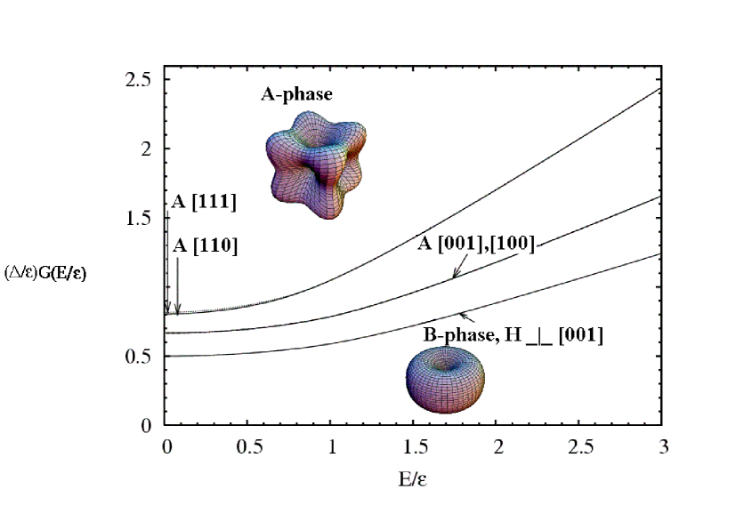
Figure 1: The functions G${}_{A}(E,{\bf H})$ and G${}_{B}(E,{\bf H})$ along various directions of the applied magnetic field.

In Fig. 1 G${}_{A}(E,{\bf H})$ is shown for ${\bf H}\parallel[111],{\bf H}\parallel[110]$ and ${\bf H}\parallel[100]$ and G${}_{B}(E,{\bf H})$ for ${\bf H}\perp[001]$. Along specific field directions we obtain

$$G_{A}(E,{\bf H}) = \frac{2\epsilon}{3\Delta}g\left(\sqrt{\frac{3}{2}}E/\epsilon\right),\mathrm{\,for\,\,{\bf H}\parallel[111]},$$ (13)

$$= \frac{\epsilon}{3\Delta}(g(\sqrt{2}E/\epsilon)+g(E/\epsilon)),\mathrm{\,for\,\,{\bf H}\parallel[110]},$$ (14)

$$= \frac{2\epsilon}{3\Delta}g(E/\epsilon),\mathrm{\,for\,\,{\bf H}\parallel[110]},$$ (15)

where $\epsilon=\frac{v}{2}\sqrt{eH}$. Note that G${}_{A}(E,{\bf H})$ for ${\bf H}\parallel[111]$ and ${\bf H}\parallel[110]$ look very similar. Also due to the cubic symmetry of $|\Delta({\bf k})|$ in the A phase (see the insert in Fig. 1) the cases ${\bf H}\parallel[111]$, ${\bf H}\parallel[-111]$ and ${\bf H}\parallel[1-11]$ etc. are equivalent.

In the B phase, the specific heat, the spin susceptibility, the superfluid density, and the nuclear spin lattice relaxation rate are then given by

$$C_{s}(T,{\bf H})/\gamma_{S}T = \frac{1}{2}\frac{\epsilon}{\Delta}f(T/\epsilon)$$ (16)

$$\chi_{s}(T,{\bf H}) = \frac{1}{2}\frac{\epsilon}{\Delta}h(T/\epsilon)$$ (17)

$$\rho_{s\parallel}(T,{\bf H})/\rho_{s}(0,0) = 1-\frac{3\epsilon}{2\Delta}h(T/\epsilon)$$ (18)

$$T_{1}^{-1}(T,H)/T_{1N}^{-1} = (\frac{\epsilon}{2\Delta})^{2}J(T/\epsilon),$$ (19)

where $\epsilon=\epsilon_{3}$ and $\rho_{s\parallel}$ denotes the current parallel to the nodes (i.e. J $\parallel[001]$). This expressions contain further scaling functions,

$$f(T/\epsilon) = \frac{3}{2\pi^{2}}(\frac{\epsilon}{T})^{3}\int_{0}^{\infty}ds\,s^{2}g(s)\mathrm{sech}^{2}\left(\frac{\epsilon s}{2T}\right)$$ (20)

$$h(T/\epsilon) = \frac{\epsilon}{2T}\int_{0}^{\infty}ds\,g(s)\mathrm{sech}^{2}\left(\frac{\epsilon s}{2T}\right)\mathrm{and\,\,}$$ (21)

$$J(T/\epsilon) = \frac{\epsilon}{2T}\int_{0}^{\infty}ds\,s\,g^{2}(s)\mathrm{sech}^{2}\left(\frac{\epsilon s}{2T}\right)$$ (22)

These expressions can be expanded in the low-temperature and high-temperature limits, with asymptotics given by

$$f(T/\epsilon) = 1+\frac{7\pi^{2}}{30}(T/\epsilon)^{2}+\ldots,\mathrm{\,for\ \ T/\epsilon\ll 1}$$ (23)

$$= \frac{27\zeta(3)}{4\pi}\frac{T}{\epsilon}+\frac{3}{4\pi}\ln(2)\frac{\epsilon}{T}+\ldots\mathrm{\,\,for\,\,\frac{T}{\epsilon}\gg 1}$$ (24)

$$h(T/\epsilon) = 1+\frac{\pi^{2}}{18}(T/\epsilon)^{2}+\ldots,\mathrm{for\,\,T/\epsilon\ll 1}$$ (25)

$$= \frac{\pi\ln 2}{2}\frac{T}{\epsilon}+\frac{\pi}{32}\frac{\epsilon}{T}\ln\left(1+(\frac{2T}{\epsilon})^{2}\right)+\ldots,\mathrm{\,\,for\,\frac{T}{\epsilon}\gg 1}$$ (26)

$$J(T/\epsilon) = 1+\frac{\pi^{2}}{9}\left(\frac{T}{\epsilon}\right)^{2}+\ldots,\mathrm{\,for\,T/\epsilon\ll 1}$$ (27)

$$= (\frac{\pi}{4})^{2}\left(\frac{1}{3}(\frac{\pi T}{\epsilon})^{2}\right)+\ldots,\mathrm{for\frac{T}{\epsilon}\gg 1}$$ (28)

These scaling functions are the same as in d-wave superconductors 14 and are shown in Fig. 2, where we introduced $F=f-\frac{27\zeta(3)T}{4\pi\epsilon}$, $K=h-\frac{\pi\ln 2}{2}\frac{T}{\epsilon}$ and $G=J-\frac{\pi^{4}}{48}(\frac{T}{\epsilon})^{2}$.

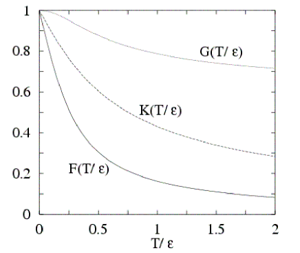
Figure 2: The scaling functions F(T/$\epsilon$), G(T/$\epsilon$), and K(T/$\epsilon$).

In analogy, for the A phase Eqs. (16), (17) and (18) are replaced by 28

$$C_{s}(T,{\bf H})/\gamma_{S}T = \frac{1}{3\Delta}\sum_{i=1}^{3}\epsilon_{i}f(T/\epsilon_{i})$$ (29)

$$\chi_{s}(T,{\bf H}) = \frac{1}{3\Delta}\sum_{i=1}^{3}\epsilon_{i}h(T/\epsilon_{i})$$ (30)

$$\rho_{s\parallel}(T,{\bf H})/\rho_{s}(0,0) = 1-\frac{1}{3\Delta}\sum_{i=1}^{3}\epsilon_{i}h(T/\epsilon_{i})$$ (31)

3. Thermal Conductivity

In order to determine the thermal conductivity it is necessary to include the effect of impurity scattering because unlike the thermodynamic response functions treated in the previous section, the scaling function for the thermal conductivity depends on the strength of the disorder, i.e. whether the impurity scattering is in the Born limit or the unitary limit 12 . As we shall see below, the scaling functions for PrOs₄Sb₁₂ turn out to be particularly simple if the heat current is parallel to a pair of point nodes. On the other hand, in the B phase the heat current has to be parallel to the nodal directions, in order to see an appreciable heat current. It appears that this condition is realized experimentally as reported in 6 . Otherwise the thermal conductivity would be much smaller since it vanishes like $T(\frac{T}{\Delta})^{2}$ as T approaches zero. In the A phase the heat current is always appreciable, although the thermal conductivity loses the cubic symmetry in the vortex state, unless H is directed along some symmetric direction (for example, ${\bf H}\parallel[111],[-111],$ etc.).

Following the derivation of Refs. 23 ; 24 , the thermal conductivity is given by

$$\kappa_{zz} = \frac{3n}{4mT^{2}}\int_{0}^{\infty}d\omega\,\omega^{2}\left\langle\frac{z^{2}h(\omega,{\bf H})}{\tilde{\Gamma}(\omega,{\bf H})}\right\rangle\mathrm{sech}^{2}(\omega/2T)$$ (32)

where

$$h = \frac{1}{2}\left(1+\frac{|\tilde{\omega}-{\bf v}\cdot{\bf q}|^{2}-\Delta^{2}f^{2}}{|(\tilde{\omega}-{\bf v}\cdot{\bf q})^{2}-\Delta^{2}f^{2}|}\right)$$ (33)

and

$$\tilde{\Gamma} = \mathrm{Im}\sqrt{(\tilde{\omega}-{\bf v}\cdot{\bf q})^{2}-\Delta^{2}f^{2}}$$ (34)

Here $<...>$ denotes the averages over the Fermi surface and vortex lattice 13 . In the superclean limit $((\Gamma\Delta)^{1/2}<\omega,|{\bf v}\cdot{\bf q}|<\Delta)\,\tilde{\omega}$ is given by

$$\tilde{\omega} = \omega+i\Gamma\left\langle\frac{|\tilde{\omega}-{\bf v}\cdot{\bf q}|}{\sqrt{(\tilde{\omega}-{\bf v}\cdot{\bf q})^{2}-\Delta^{2}f^{2}}}\right\rangle$$ (35)

$$\simeq \omega+i\Gamma G(\omega,{\bf H})$$ (36)

in the Born limit. And in the unitary limit we find

$$\tilde{\omega}=\omega+i\Gamma G^{-1}(\omega,{\bf H})$$ (37)

where G($\omega,{\bf H}$) for the A and B phase have been defined in Eqs. (5) and (6).

Let us first consider the Born limit. Substituting Eq.(35) into Eq.(32) we obtain

$$\kappa_{zz} = \frac{3n}{8mT^{2}\Gamma}\int_{0}^{\infty}d\omega\,\omega^{2}\frac{<|\omega-{\bf v}\cdot{\bf q}|>^{{}^{\prime}}}{<|\omega-{\bf v}\cdot{\bf q}|>}\mathrm{sech}^{2}(\omega/2T)$$ (38)

where $<|\omega-{\bf v}\cdot{\bf q}|>^{{}^{\prime}}$ is the same as $<|\omega-{\bf v}\cdot{\bf q}|>$ but with contributions from nodes at (001) and (00 -1) only. Then in the B phase $<|\omega-{\bf v}\cdot{\bf q}|>^{{}^{\prime}}=<|\omega-{\bf v}\cdot{\bf q}|>\,\,$ and thus $\kappa^{B}_{zz}=\frac{3}{2}\kappa_{n}$, where $\kappa_{n}=\frac{\pi^{2}Tn}{6m\Gamma}$ is the thermal conductivity in the normal state. The thermal conductivity in the Born limit is independent of H. On the other hand in the A phase$\,\,<|\omega-{\bf v}\cdot{\bf q}|>^{{}^{\prime}}\neq<|\omega-{\bf v}\cdot{\bf q}|>$, leading to

$$\kappa_{zz}^{A}/\kappa_{n} = \frac{1}{2},\mathrm{\ \ \ for\,\,\,T\gg\epsilon},$$ (39)

$$= \frac{3}{2}\epsilon_{3}/(\epsilon_{1}+\epsilon_{2}+\epsilon_{3}),\mathrm{\,\,for\,\,T\ll\epsilon}.$$ (40)

The $\epsilon_{i}$’s were defined in Eq.(9).

The scaling law is of greater interest in the unitary limit. First let us consider the B phase where $<|\omega-{\bf v}\cdot{\bf q}|>^{{}^{\prime}}=<|\omega-{\bf v}\cdot{\bf q}|>$. Substituting Eq. (37) into Eq. (32) one obtains

$$\kappa_{zz}^{B} = \frac{3\pi^{2}n}{512m\Gamma(T\Delta)^{2}}\int_{0}^{\infty}\ d\omega\omega^{2}<|\omega-{\bf v}\cdot{\bf q}|>^{2}\mathrm{sech}^{2}(\omega/2T)$$ (41)

$$= \frac{3n\epsilon^{5}}{32m\Gamma(T\Delta)^{2}}\int_{0}^{\infty}\ ds\,s^{2}g^{2}(s)\mathrm{sech}^{2}(\epsilon s/2T)$$ (42)

and the scaling function is defined as

$$F(T/\epsilon)\equiv\frac{\kappa_{zz}^{B}(T,{\bf H})}{\kappa_{zz}^{B}(T,0)}=\frac{120}{\pi^{6}}(\frac{T}{\epsilon})^{-6}\int_{0}^{\infty}\ ds\,s^{2}g^{2}(s)\mathrm{sech}^{2}(\epsilon s/2T)$$ (43)

where $\epsilon=\epsilon_{3}$.

Figure 3: The scaling function F(T/$\epsilon$) for the unitary limit (U), the Born limit (B) and the case without inversion symmetry (I) are shown as a function of T/$\epsilon$.

where $\epsilon=\epsilon_{3}$. This scaling function is shown in Fig. 3, with asymptotics given by

$$\kappa_{zz}^{B}/\kappa_{n} = \frac{21\pi^{4}}{640}(\frac{T}{\Delta})^{2}\left(1+\frac{5}{7}(\frac{\epsilon}{\pi T})^{2}+\ldots\right),\,\,\mathrm{for\,\,\epsilon\ll T}$$ (44)

$$= \frac{3\pi^{2}}{8}(\frac{\epsilon}{\Delta})^{2}\left(1+\frac{7\pi^{2}}{15}(\frac{T}{\epsilon})^{2}+\ldots\right),\,\,\mathrm{for\,\epsilon\gg T}$$ (45)

and

$$F^{B}(T/\epsilon) = 1+\frac{5}{7}\left(\frac{\epsilon}{\pi T}\right)^{2}+\ldots,\,\,\mathrm{for\,\epsilon\ll T}$$ (46)

$$= \frac{80}{7\pi^{4}}(\frac{\epsilon}{\Delta})^{2}\left(1+\frac{7\pi^{2}}{15}(\frac{T}{\epsilon})^{2}+\ldots\right),\,\,\mathrm{for\,\epsilon\gg T}$$ (47)

This scaling function $F(T/\epsilon)$ is the same in other nodal superconductors such as those with d-wave symmetry. For example, $F^{B}(T/\epsilon)$ describes very well the scaling behavior recently observed by Suderow et al 18 in UPt₃.

In the A phase the scaling function is somewhat more complicated. We find

$$\kappa_{zz}^{A} = \frac{n\epsilon_{3}}{72m\Gamma(\Delta T)^{2}}\int_{0}^{\infty}\,d\omega\,\omega^{2}\,g(\omega/\epsilon_{3})\left(\sum_{i=1}^{3}\epsilon_{i}g(\omega/\epsilon_{3})\right)\,\mathrm{sech}^{2}(\omega/2T)$$ (48)

In particular for ${\bf H}\parallel[111]$ and $[100]$ Eq.(48) reduces to

$$\kappa_{zz}^{A} = \frac{n\epsilon_{3}^{5}}{24m\Gamma(\Delta T)^{2}}\int_{0}^{\infty}\,ds\,s^{2}\,g^{2}(s)\mathrm{sech}^{2}\left(\epsilon_{3}s/2T\right)\mathrm{\,for\,{\bf H}\parallel[111],\,\,and}$$ (49)

$$= \frac{n\epsilon_{3}^{5}}{36m\Gamma(\Delta T)^{2}}\int_{0}^{\infty}\,ds\,s^{2}\,g^{2}(s)\mathrm{sech}^{2}\left(\epsilon_{3}s/2T\right)\mathrm{\,for\,{\bf H}\parallel[100]}$$ (50)

where $\epsilon_{3}=\frac{v\sqrt{eH}}{2}\sqrt{\frac{2}{3}}$ and $\frac{v\sqrt{eH}}{2}$ for ${\bf H}\parallel[111]$ and ${\bf H}\parallel[100]$ respectively. Therefore in these two cases we will have the same scaling function as $F^{B}(T/\epsilon)$.

4. Concluding Remarks

We conclude that the scaling behavior of the universal heat conduction and the thermal conductivity can be regarded as a hallmark of nodal superconductivity 22 . Moreover, the scaling function $F^{B}(T/\epsilon)$ describes the thermal conductivity data measured in UPt₃ by Suderow et al 18 very well. In this paper, we have found that the thermal conductivity in both the A and B phases of PrOs₄Sb₁₂ exhibits a number of characteristic scaling relations. The directional dependence of these scaling relations on ${\bf H}$ and ${\bf q}$ is expected to further confirm the nodal structure of $\Delta({\bf k})$ proposed in 6 .

In the course of the present study we have also observed that the scaling behavior of the thermal conductivity in CePt₃Si found by Izawa et al 25 ; 26 is very unusual. Their data appears to be more consistent with the case where the inversion symmetry of the impurity scattering is broken. Clearly, further study of scaling laws in nodal superconductors will open a new point of view on the whole subject.

Acknowledgements

We thank K. Izawa and Y. Matsuda for sharing with us unpublished data of the thermal conductivity in CePt₃Si, which gave a strong motivation for the present analysis. HW acknowledges support from the Korean Science and Engineering Foundation (KOSEF) through grant number R05-2004-000-10814, while SH acknowledges support from the National Science Foundation through grant number DMR-0089882.

References

(1)
(2) E.D. Bauer, N.A. Frederick, P.-C. Ho, V.S. Zapf and M.B. Maple,
Phys. Rev. B 65, R100506 (2002).
(3) R. Vollmer, A Fait, C. Pfleiderer, H. v. L hneysen, E. D. Bauer, P.-C. Ho, V. Zapf, and M. B. Maple, Phys. Rev. Lett. 90, 57001 (2003).
(4) H. Kotegawa, M. Yogi,Y. Imamura, Y. Kawasaki, G.-q. Zheng, Y. Kitaoka, S. Ohsaki, H. Sugawara, Y. Aoki, and H. Sato, Phys. Rev. Lett.
90, 027001 (2003).
(5) K. Izawa, Y. Nakajima, J. Goryo, Y. Matsuda, S. Osaki, H. Sugawara, H. Sato, P. Thalmeier, and K. Maki, Phys. Rev. Lett. 90, 117001 (2003).
(6) Y. Aoki, A. Tsuchiya, T. Kanayama, S. R. Saha, H. Sugawara, H. Sato,
W. Higemoto, A. Koda, K. Ohishi, K. Nishiyama, and R. Kadono, Phys. Rev. Lett.
91, 067003 (2003).
(7) K. Maki, S. Haas, D. Parker, H. Won, K. Izawa and Y. Matsuda, Europhys.
Lett. 68, 720 (2004).
(8) M.-A. Measson, D. Braithwaite, J. Flouquet, G. Seyfarth, J. P. Brison, E. Lhotel, C. Paulsen, H. Sugawara, and H. Sato, Phys. Rev. B 70, 064516 (2004).
(9) D. Parker, K. Maki and S. Haas, cond-mat/0407254.
(10) S.H. Simon and P.A. Lee, Phys. Rev. Lett. 78, 1548 (1997).
(11) G.E. Volovik, JETP Lett. 58, 469 (1993).
(12) C. Kübert and P.J. Hirschfeld, Solid State Comm.
105, 459 (1998).
(13) C. Kübert and P.J. Hirschfeld, Phys. Rev. Lett.
80, 4963 (1998).
(14) H. Won and K. Maki, cond-mat/0004105.
(15) H. Won and K. Maki, Europhys. Lett. 54, 248 (2001).
(16) H. Won and K. Maki, Europhys. Lett. 56, 729 (2001)
(17) B. Revaz, J.-Y. Genoud, A. Junod, K. Neumaier, A. Erb, and E. Walker,
Phys. Rev. Lett. 80, 3364 (1998).
(18) K. Deguchi, Z.Q. Mao and Y. Maeno, J. Phys. Soc. Jpn. 75, 1315
(2004).
(19) H. Suderow, J. P. Brison, A. Huxley, and J. Flouquet, Phys. Rev. Lett. 80, 165 (1998).
(20) Note that in this paper we do not consider the
proposed s+g-wave superconductor
YNi2B2C 19 ; 20 ; 21 .
The presence of an s-wave component in the order
parameter of this material spoils both the universal heat conduction and
the scaling relation.
(21) H. Won, S. Haas, D. Parker, S. Telang, A. Vanyolos, and K. Maki in
Proceedings of Ninth Training School at Vietri sul Mare, Italy, 2005;
also cond-mat/0501463.
(22) The expression of for the A-phase is somewhat more involved.
(24) V. Ambegaokar and A. Griffin, Phys. Rev. 137, A1151 (1965).
(25) E. Bauer, G. Hilscher, H. Michor, Ch. Paul, E. W. Scheidt, A. Gribanov, Yu. Seropegin, H. Noël, M. Sigrist, and P. Rogl, Phys. Rev. Lett. 92,
027003 (2004).
(26) K. Izawa, K. Behnia, K. Kasahara, M. Isaki, Y. Matsuda. K. Yasuda,
R. Settai, Y. Onuki (private communication).
(27) K. Maki, P. Thalmeier and H. Won, Phys. Rev. B 65, 140502R (2002).
(28) K. Izawa, K. Kamata, Y. Nakajima, Y. Matsuda, T. Watanabe, M. Nohara, H. Takagi, P. Thalmeier, and K. Maki, Phys. Rev. Lett. 89, 137006 (2002).
(29) Q. Yuan, H.-Y. Chen, H. Won, S. Lee, K. Maki, P. Thalmeier, and C. S. Ting, Phys. Rev. B 68, 174510 (2003)