Log-periodic oscillations in degree distributions of hierarchical scale-free networks

Abstract

Hierarchical models of scale free networks are introduced where numbers of nodes in clusters of a given hierarchy are stochastic variables. Our models show periodic oscillations of degree distribution $P(k)$ in the log-log scale. Periods and amplitudes of such oscillations depend on network parameters. Numerical simulations are in a good agreement to analytical calculations.

89.75.Hc, 89.75.-k, 89.75.Da, 89.75.Fb

1 Introduction

Recently there is a large interest in scale-free networks that seem to be good approximations for such systems as the Internet, World Wide Web, social or biological networks; for a review see [1]-[4]. A simple model that exhibits the power law for degree distributions $P(k)$ observed in real complex networks is the Barabási-Albert model of preferential attachment [1]. The model however suffers from very low values of the clustering coefficient $C$ [5] for large networks as compared to observations of real systems [1]-[4]. To overcome this discrepancy a model of hierarchical networks has been introduced by Ravasz and Barabási (RB) where the clustering coefficient is much larger [6]. The RB network consists of hierarchically connected clusters where numbers of nodes in every cluster of a given hierarchy are the same. The degree distribution $P(k)$ in this approach also exhibits power-law. However, it is only a general trend. In fact, the degree distribution consists of delta-peaks for only a few degree values, instead of continuous distribution observed in real networks. In this paper, we introduce a class of more general models, where number of nodes in every cluster is a stochastic variabl, what seems to be more justified for real network models. As result the peaks of $P(k)$ are blurred, creating a network with wide range of possible $k$ values, but the log-periodic behaviour of $P(k)$ is still clearly visible.
Let us remind that log-periodic oscillations are characteristic features of systems where a discrete self-similarity is present [7] and the effect can occur even without a preexisting hierarchy [7] in such various systems as earthquakes [8, 9] or financial markets where log-periodic oscillations were observed as possible precursors for financial crashes [10, 11, 12]. Such oscillations were also found for mean residence times at chaotic crisis where a collision of a fractal attractor with a fractal or a nonfractal basin of another attractor takes place [13, 14] and for the stochastic resonance in chaotic systems near a crisis point [15].

2 The Model

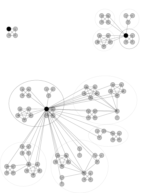
Figure 1: The first three steps of network creation in the P1 model.

Our model possesses two parameters, a distribution $P_{M}(m)$, where $m=1,2,3,\dots$ and a number $p\in(0,1]$. We start out from a single cluster (a cluster of hierarchy $0$) of $m+1$ fully connected nodes (Fig.1), where $m$ is a random number from a distribution $P_{M}(m)$. One node in the cluster is its central node. The central node of the cluster is a center of hierarchy $0$. Next, we call our cluster the central one and create a random number $m$ of similar clusters. Each is created in the same way as the central cluster, but we pick a random number $m$ for each one independently, therefore they may include different numbers of nodes. Next, we connect a part $p$ of all nodes in non-central clusters to the central node in the central cluster. This node becomes the central node for the whole cluster of hierarchy $1$ we have obtained so far. Similarly the central node of our cluster is a center of hierarchy $1$. We repeat the process, until we get a network of a desired hierarchy. This model is referred to as P1 model. The model is generalization of the stochastic model proposed by Barabási and Ravasz [6]. If we take $P_{M}(m)=\delta(m,m_{0})$, where $m_{0}$ is constant, our model simplifies to BR model, with number of nodes and degree distribution determined strictly by $p$ and $m_{0}$ values.

A variation of the model has been also studied. In each hierarchy $d$ we connect not a fraction $p$ of nodes but a fraction $p^{d}$. This model is referred to as the PD model.

3 Degree Distribution of P1 and PD models

As previously noted, for $P_{M}(m)=\delta(m,m_{0})$ we get a degree distribution identical to that of BR model. It consists of separate peaks, corresponding to degrees of central nodes of following hierarchies. Central nodes of given hierarchy have a fixed degree, dependent only on the network parameter $p$. At the logarithmic scale the distance between neighboring peaks is approximately constant and equals to $\log(m_{0}+1)$. The peaks follow laws of discrete scaling [7]. The heights of peaks with degrees $k_{i}$ decrease as $k_{i}^{-\gamma}$, and distances between consecutive peaks fulfill the relation $k_{i+1}/k_{i}=\lambda$. The probability $P(k)$ between peaks equals to zero what means that only nodes with peculiar degrees are possible. But what happens when the number $m$ is not a fixed value ?
Numerical simulations show that each peak blurs, depending on the $P_{M}(m)$ distribution. If the blur is small, the distribution consists of separate peaks, but they are not delta-shaped. If the blur is large enough, the peaks overlap and a continuous degree distribution is obtained. Figure 2 shows degree distributions for both cases in P1 model. Both display a discrete scaling, and have the same scaling exponent (up to statistical fluctuations), independent on network parameters.
Similar behavior has been observed in the PD model, although scaling exponent is parameters dependent.

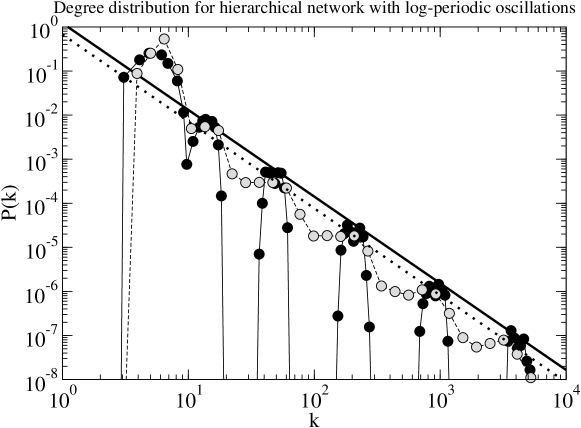
Figure 2: Degree distribution for two networks with different $P_{M}(m)$. Filled circles are for $m=3$ or $4$ with equal probability, gray circles are for uniform $m$ distribution between $1$ and $5$. The straight lines show scaling of peak heights and correspond to $\gamma=0.967$ for the first case (continuous line) and $\gamma=0.973$ for the second (dotted line).

4 Mean $m$ value approach

Numerical simulations have shown that when $m$ is not a constant but a random number from a given distribution, peaks blur, eventually overlapping and creating a continuous distribution. However, regardless of the actual shape, the distribution still consists of peaks. Each peak has an average degree $k$ and a mass $n$ representing number of nodes that belong to this peak. All nodes in a peak are centers of the same hierarchy. Using a mean value of $m$, the distance between peaks and their relative heights can be easily found. From these two values we directly get the discrete scaling ratio $\lambda$ and the scaling exponent $\gamma$. In the following calculations we neglect the degree increase of nodes due to their connections to the central cluster, as this effect increases the node degree at most by $d$, what is insignificant for higher hierarchy centers.

4.1 P1 model

Let us denote an average degree of peak of hierarchy $d$ by $k_{d}$, an average number of nodes in a cluster of hierarchy $d$ by $N_{d}$, and an average number of centers of hierarchy $d$ in a network of hierarchy $h$ by $n_{d}^{h}$. The network size $N_{d}$ increases exponentially with hierarchy $d$ as $N_{d}=\left\langle m+1\right\rangle^{d+1}$. Centers of hierarchy $0$ have a degree $k_{0}$ equal to $\left\langle m\right\rangle$ and it increases by $p\cdot\left\langle m\right\rangle\cdot N_{d-1}$ in each next hierarchy $d$. We obtain

$$k_{d}=\left\langle m\right\rangle+p\cdot\left\langle m+1\right\rangle\cdot\left(\left\langle m+1\right\rangle^{d}-1\right)$$ (1)

If $\left\langle m+1\right\rangle>1$ and $d>>1$, the above expression can be simplified to

$$k_{d}\approx p\cdot\left\langle m+1\right\rangle^{d+1}$$ (2)

If the condition is not satisfied, distances between peaks are not constant at logarithmic scale and the network is not scale-free.

Since the discrete scaling ratio $\lambda$ simply equals $k_{d+1}/k_{d}$ thus we get $\lambda\approx\left\langle m+1\right\rangle$.

The scaling exponent $\gamma$ can be found using the cumulative degree distribution. Starting from

$$P(k)=\frac{\Delta P_{cum}}{\Delta k}=\frac{\Delta P_{cum}}{\Delta d}\frac{\Delta d}{\Delta k}$$ (3)

where $d$ are consecutive hierarchies, and using calculations presented in Appendix A we get $P(k)\sim k^{-2}$ so the scaling exponent $\gamma$ equals to $2$, regardless of $p$ and $P_{M}(m)$. Note that this scaling is valid for peak masses $n_{d}^{h}$ only.

4.2 PD Model

The case of PD model is very similar to the P1 model. However, since instead of a fraction $p$ we connect a fraction $p^{d}$ of nodes from non-central clusters, the degree $k_{d}$ is

$$k_{d}=\left\langle m\right\rangle\frac{1-(p\cdot\left\langle m+1\right\rangle)^{d+1}}{1-p\cdot\left\langle m+1\right\rangle}$$ (4)

When we assume that $p\cdot\left\langle m+1\right\rangle>1$ we can omit one in the numerator and get the discrete scaling ratio $\lambda=k_{d+1}/k_{d}\approx p\cdot\left\langle m+1\right\rangle$. Similarly to the P1 model, if it is not true, the network is not scale-free.

To find the scaling exponent, again we use cumulative degree distribution and Eq.3. For the PD model we get $\gamma=1+\frac{\ln\left\langle m+1\right\rangle}{\ln p\left\langle m+1\right\rangle}$. Note that since $p\in(0,1]$ and $p\left\langle m+1\right\rangle>1$ for scale-free networks, the scaling exponent is always greater than $2$.

4.3 Numerical Data

Numerical simulations have been performed for networks of hierarchy $6$, with $p=0.5$ and various uniform distributions of $m$, to find out if analytic predictions are correct.

Tables 1 and 2 contain obtained data. Figure 3 shows the comparison between prediction and results.

As it can be seen the numerical data are in a good agreement with our analytic predictions. The largest deviation is for low $\left\langle m\right\rangle$ and for low $p$, where our approximations were poor.

$m$	$\left\langle m+1\right\rangle$	$\gamma_{analyt}$	$\gamma_{numer}$	$\log\lambda_{analyt}$	$\log\lambda_{numer}$
1 to 2	2.5	2	1.981	0.398	0.397
1 to 3	3	2	1.978	0.477	0.461
1 to 4	3.5	2	1.931	0.544	0.556
1 to 5	4	2	1.973	0.602	0.606

Table 1: Distribution of $m$ numbers, analytic and numerical scaling exponents $\gamma$ and the logarithm of discrete scaling ratio $\lambda$ for the model P1. Data obtained from averaging over $30$ networks.

$m$	$\left\langle m+1\right\rangle$	$\gamma_{analyt}$	$\gamma_{numer}$	$\log\lambda_{analyt}$	$\log\lambda_{numer}$
1 to 2	2.5	5.106	3.858	0.097	$\sim$0.16
1 to 3	3	3.710	3.067	0.176	0.208
1 to 4	3.5	3.239	3.038	0.243	0.271
1 to 5	4	3.000	2.846	0.301	0.32

Table 2: Distribution of $m$ numbers, analytic and numerical scaling exponents $\gamma$ and the logarithm of discrete scaling ratio $\lambda$ for the model PD. Data obtained from averaging over $2000$ networks. In the first row, the exact $\lambda$ value was impossible to obtain, due to very weak periodic behavior.

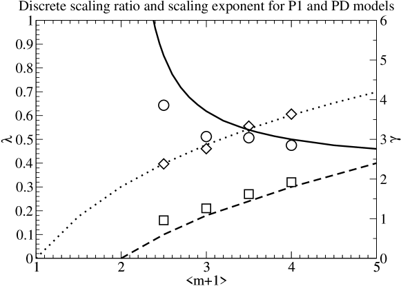
Figure 3: The discrete scaling ratio $\lambda$ and the scaling exponent $\gamma$. Symbols are values obtained from numeric simulations, lines are analytic predictions. Diamonds and dotted line are for $\lambda$ in P1 model. Squares and dashed line are for $\lambda$ in PD model. Circles and smooth line are for $\gamma$ in PD model. In all cases, networks are of hierarchy $6$, with parameter $p=0.5$.

5 Exact degree distribution

Up to now, all calculations have been performed using only the average $m$ value, treating the degree distribution as series of peaks. We have been concentrating on relations between peak’s masses and distances, while ignoring their shape. Here we find a shape of the degree distribution for the P1 model.
Let $P_{M}(m)$ be a distribution of $m$, where $m$ is a number of noncentral clusters in each hierarchy. Let $\widetilde{P}_{d}(N)$ be a distribution of the network sizes $N$ for hierarchy $d$. $P_{d}(k)$ is a degree distribution for a network of hierarchy $d$, $P_{d}^{c}(k)$ is a degree distribution for the central node of hierarchy $d$.

The number of nodes in the network can be found as follows. Network of hierarchy $d=0$ has $m+1$ nodes what means $\widetilde{P}_{0}(N)=P_{M}(N-1)$. The size of each next hierarchy $d+1$ is a sum of $m+1$ independent values, which are sizes of networks of hierarchy $d$.

$$\widetilde{P}_{d+1}(N)=\sum_{m}P_{M}(m)\sum_{n_{1},n_{2},\dots,n_{m}}\widetilde{P}_{d}(n_{1})\widetilde{P}_{d}(n_{2})\dots\widetilde{P}_{d}(N-n_{m}-\dots-n_{1})$$ (5)

This recursive formula describes the probability distribution for the network size $N$.

A network of hierarchy $d=0$ has degree distribution $P_{0}(k)=P_{M}(k)$. This distribution describes both regular nodes and a center of hierarchy $0$, which have the same degree values. In each next hierarchy $d+1$ the degree distribution for all nodes of hierarchy $d$ or less is the same, since we omit the degree increase due to connections to the central node of higher hierarchy. Now, we multiply the distribution by $(m+1)$ and add the degree distribution $P_{d+1}^{c}(k)$ for the central node of the network. This way we obtain an unnormalized degree distribution for the whole network of hierarchy $d+1$.

$$P_{d+1}(k)=\sum_{m}\left[(m+1)P_{M}(m)P_{d}(k)+P_{d+1}^{c}(k)\right]$$ (6)

The center is roughly connected to fraction $p$ of all nodes in the network, what means it possesses the degree $p\cdot N$. This yields the distribution of its degree equal to $P_{1}^{c}(k)=\widetilde{P}_{1}(k/p)$. As result we obtain

$$P_{d+1}(k)=\sum_{m}\left[(m+1)P_{M}(m)P_{d}(k)+\widetilde{P}_{d+1}(k/p)\right]$$ (7)

This recursive formula describes the unnormalized degree distributions for networks of consecutive hierarchies $d$, with the exception of $d=1$. Since $P_{0}(k)$ describes not only centers of hierarchy $0$ but both regular nodes and centers, we must account for that. We do so by multiplying $P_{0}(k)$ in the formula by the average basic cluster size $\left\langle m+1\right\rangle$.

$$P_{1}(k)=\sum_{m}\left[\left\langle m+1\right\rangle(m+1)P_{M}(m)P_{0}(k)+\widetilde{P}_{1}(k/p)\right]$$ (8)

In the above calculations, like in the calculations using average $m$, we omitted the degree increase due to connections to the central node of higher hierarchy. This is insignificant for higher hierarchy centers, as the increase is at most $d$, while the center degree increases exponentially with $d$. We have used the formula $P_{d}^{c}(k)=\widetilde{P}_{d}(k/p)$ in the above calculations. In reality degree distributions are discrete, with natural $k$ values. Depending on how we round the number of connections to the central node, we should interpret the above formula accordingly.

We rounded the number of connections $p\cdot N$ down, what gives the following formula for interpreting the probability with fractional argument

$$P_{d}^{c}(k)=\sum_{l\geq k/p,l<(k+1)/p}\widetilde{P}_{d}(l)$$ (9)

It means that the probability of getting the center of degree $k$ equals to the sum of probabilities for $N$, that lead to this $k$. Along with

$$\widetilde{P}_{0}(N)=P_{M}(N-1)$$ (10)

and

$$P_{0}(k)=P_{M}(k)$$ (11)

Eqs.5 and 7-9 allow to find numerically an exact but unnormalized degree distribution for the P1 model.

Comparing these formulas with numerical data one can see that our calculations are correct for higher degrees, where approximations we used are accurate (Fig.5, Fig.4).

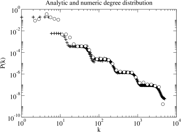
Figure 4: Degree distribution for the network with uniform $m$ distribution from $1$ to $5$, and hierarchy $d=5$. The graph shows analytic (crosses) and numeric data (circles).

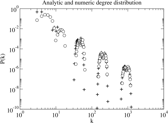
Figure 5: The degree distribution for network with the uniform $m$ distribution ($3$ or $4$), and the hierarchy $d=4$. The graph shows analytic (crosses) and numeric data (circles).

Using degree distributions obtained with our formulas (Eq.5,Eqs.7-11), a relation between the distribution of $m$ and a peak shape has been found. We have studied various uniform distributions of $m$ and have found linear relation between the standard deviation of the distribution $P(\ln m)$ and the standard deviation of peaks in the $P(\ln k)$ distribution (Fig.6).

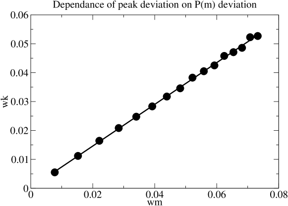
Figure 6: Relation between the peak width $wk$ (a standard deviation of peaks in $P(\ln k)$) and the distribution width $wm$ (a standard deviations of $P(\ln m)$). The slope of the line is $\alpha=0.722$.

Peak deviations in the distribution P(k) are calculated at the logarithmic scale of $k$

$$\sigma=\frac{\sum(\ln k-\left\langle\ln k\right\rangle)^{2}\cdot P(\ln k)}{\sum P(\ln k)}$$ (12)

Similar formula has been used to calculate the deviation of $P(m)$. Peak deviations have been calculated for the peak of the highest hierarchy. In the case of overlapping peaks the minimums of $P(k)$ have been considered borders of peak. The approximation is quite accurate, as $P(k)$ decays fast when we go away from the peak average $k$ value.

6 Discussion

The question occurs, whether our model corresponds to real network systems. It is obvious that many real networks posess a hierarchical structure but of course a detailed mechanism responsible for its emergence is unknown. According to our knowledge, log-periodic oscillations around the power law in degree distributions were never directly reported in the studies of real networks or corresponding models. One can suspect however, that in many cases such oscillations were visible and could be overlooked if the binning or data averaging had been performed. Small amplitude oscillations can be also easily confused with random fluctuations. The situation resembles oscillations around the scaling law in chaotic crises, where the periodic part is also often omitted as fluctuations [13, 14].
A clear example of log-periodic oscillations for real networks can be seen in the study of liability connections between Austrian banks [16]. As the authors stress [16] a significant part of studied banking sector posesses a strong hierarchical structure, what can be easily detected looking at a corresponding connection graph. Two periods of oscillations can be identified at out-degree distribution describing the number of liabilities to other Austrian banks (regardless of liability size) [16]. The period of the oscillations is approximately $\lambda=k_{i+1}/k_{i}\approx 3$. According to our theory, they are a result of the network’s hierarchical structure.
We have found also far less visible oscillations in the studies of computer directory trees [17] and World Trade Web [18], where the hierarchical structure can be identified at a corresponding connection graph [17] or in dependence of a clustering coefficient on a node degree [18]. Sizes of such oscillations are however at a fluctuations level. The other possible example can be found in the paper [19], that presents a non-monotenous behavior of degree distribution of P(k) for a shareholding network in Japan. Here a single wave around the power law can be observed, where $\lambda=k_{i+1}/k_{i}\approx 10$.

7 Conclusions

In conclusion we have shown that hierarchical networks models display log-periodic oscillations in the degree distribution when the number of clusters forming the self-similar hierarchy is a stochastic variable. The period and the amplitude of these oscillations reflect the hierarchical structure of the network. We also point out examples of real networks that display such features. It follows that observations of log-periodic oscillations in degree distributions of real networks can give hints towards the existence of hidden hierarchical structures in such systems.

8 Acknowledgement

This work has been partially supported by by a special Grant Dynamics of Complex Systems of the Warsaw University of Technology and by the EU Grant Measuring and Modelling Complex Networks Across Domains (MMCOMNET).

Appendix A Mean $m$ value calculations

This Appendix contains exact calculations regarding the discrete scaling ratio $\lambda$ and the scaling exponent $\gamma$ for the mean $m$ approach. The number $k_{d}$ is an average degree of peak of hierarchy $d$, $N_{d}$ is an average number of nodes in network of hierarchy $d$, $n_{d}^{h}$ is an average number of centers of hierarchy $d$ in a network of hierarchy $h$. The number $\left\langle m+1\right\rangle$ is a mean number of clusters in each hierarchy.

The Eq.2 can be obtained as

$$k_{d}=k_{d-1}+\left\langle m\right\rangle\cdot N_{d-1}\cdot p=\left\langle m\right\rangle+p\cdot\left\langle m\right\rangle\cdot\sum^{i=1}_{d}\left\langle m+1\right\rangle^{i}=$$ (13)

$$=\left\langle m\right\rangle+p\cdot\left\langle m+1\right\rangle\cdot\left(\left\langle m+1\right\rangle^{d}-1\right)$$

The scaling exponent $\gamma$ for model P1 has been obtained using the cumulative degree distribution

$$P(k)=\frac{\Delta P_{cum}}{\Delta k}=\frac{\Delta P_{cum}}{\Delta d}\frac{\Delta d}{\Delta k}$$ (14)

First we find an expression for $n_{d}^{h}$. There is only one center of hierarchy $d=h$ in the network of such a hierarchy. Each time the network hierarchy $h$ increases, the number of centers of hierarchy $d$ increases $\left\langle m+1\right\rangle$ times. The exception is the first step, where one node becomes center of the higher hierarchy. Because of that $n_{d}^{h}$ increases only by the factor of $\left\langle m\right\rangle$ for that step. We obtain $n_{d}^{h}=\left\langle m\right\rangle\cdot\left\langle m+1\right\rangle^{h-d-1}$ except for $n_{h}^{h}=1$.

Now we calculate expressions in Eq.14. Each next peak is smaller $\frac{\Delta P_{cum}}{\Delta d}=n_{d}^{h}\sim\left\langle m+1\right\rangle^{-d}$ while its average degree $k_{d}$ increases $\frac{\Delta k}{\Delta d}\sim\left\langle m+1\right\rangle^{d}$ In such a way we obtain

$$P(k)\sim\left\langle m+1\right\rangle^{-d}\cdot\left\langle m+1\right\rangle^{-d}=\left\langle m+1\right\rangle^{-2d}$$ (15)

From Eq.13 we get $d\approx\log_{\left\langle m+1\right\rangle}\frac{k}{p}-1=\frac{\ln k-\ln p}{\ln\left\langle m+1\right\rangle}-1$. By putting so calculated $d$ into Eq.15 we get

$$P(k)\sim\left\langle m+1\right\rangle^{-2d}=\exp\left(-2d\ln\left\langle m+1\right\rangle\right)=$$ (16)

$$\exp\left(-2\frac{\ln k-\ln p}{\ln\left\langle m+1\right\rangle}\ln\left\langle m+1\right\rangle+2\ln\left\langle m+1\right\rangle\right)\sim\exp\left(-2\ln k\right)=k^{-2}$$

For the PD model the Eq.4 can be obtained in the following way

$$k_{d}=k_{d-1}+\left\langle m\right\rangle\cdot N_{d-1}\cdot p^{d}=$$ (17)

$$=\left\langle m\right\rangle\cdot\sum_{i=0}^{d}p^{i}\cdot\left\langle m+1\right\rangle^{i}=\left\langle m\right\rangle\frac{1-(p\cdot\left\langle m+1\right\rangle)^{d+1}}{1-p\cdot\left\langle m+1\right\rangle}$$

The scaling exponent has been calculated in a similar way to the case of model P1. The slope $\Delta P_{cum}/\Delta d$ is the same as in the previous case but $\Delta k/\Delta d\sim(p\cdot\left\langle m+1\right\rangle)^{d}$ thus $P(k)\sim p^{-d}\cdot\left\langle m+1\right\rangle^{-2d}$.

Expressing $d$ by $k$ we get $d=\log_{p\left\langle m+1\right\rangle}\frac{(p\cdot\left\langle m+1\right\rangle-1)\cdot k}{\left\langle m\right\rangle}-1$ and putting that into Eq.14 we get $P(k)\sim k^{-(1+\frac{\ln\left\langle m+1\right\rangle}{\ln p\left\langle m+1\right\rangle})}$ which yields exponent $\gamma=1+\frac{\ln\left\langle m+1\right\rangle}{\ln p\left\langle m+1\right\rangle}$ for PD model.

References

- [1] R.Albert, A.-L.Barabási, Rev. Mod. Phys. 74, 47-97 (2002).
- [2] M.E.J.Newman, SIAM Rev. 45, 167-256 (2003).
- [3] S.N.Dorogovtsev, J.F.F.Mendes, Evolution of Networks: From Biological Nets to the Internet and WWW (Oxford University Press, Oxford, 2003).
- [4] Handbook of Graphs and Networks, edited by S.Bornhold, H.G.Schuster (Viley-VCH, Berlin 2002).
- [5] A. Fronczak, P. Fronczak and J.A. Hołyst, Phys. Rev. E 68, 046126 (2003).
- [6] E.Ravasz, A.-L.Barabási, Phys. Rev. E 67, 026112 (2003).
- [7] D.Sornette, Phys. Rep. 297, 239-270 (1998).
- [8] D. Sornette and C.G. Sammis, J.Phys.I France 5 607 (1995).
- [9] H. Saleur, C.G. Sammis and D. Sornette, Nonlinear Processes Geophys. 3 102 (1996).
- [10] M.Ausloos, Physica A 285, 48-65 (2000).
- [11] D.Sornette, Phys. Rep. 378, 1-89 (2003).
- [12] W.X.Zhou, D.Sornette, Int.J.Mod.Phys C 14, 1107-1125 (2003).
- [13] K.Kacperski and J.A.Hołyst, Phys. Rev. E 60, 403-407 (1999).
- [14] K.Kacperski, J.A.Hołyst, Phys. Lett. A. 254, 53 58 (1999).
- [15] S.Matyjaśkiewicz, A.Krawiecki, J.A.Hołyst, K.Kacperski, W.Ebeling, Phys. Rev. E 63, 026215 (2001).
- [16] M.Boss, H.Elsinger, M.Summer, S.Thurner, ”The Network Topology of the Interbank Market”, arXiv:cond-mat/0309582
- [17] K.Klemm, V.Eguiluz, M.San Miguel, ”Information management by computer users: the structure of directory trees”, arXiv:cond-mat/0403239
- [18] M.-Á.Serrano, M.Boguñá, Physical Review E 68, 015101(R) (2003)
- [19] W.Souma, Y.Fujiwara, H.Aoyama, Physica A 344, 73-76 (2004)