On the fundamental diagram of traffic flow

Abstract

We present a new fluid-dynamical model of traffic flow. This model generalizes the model of Aw and Rascle [SIAM J. Appl. Math. 60 916-938] and Greenberg [SIAM J. Appl. Math 62 729-745] by prescribing a more general source term to the velocity equation. This source term can be physically motivated by experimental data, when taking into account relaxation and reaction time. In particular, the new model has a (linearly) unstable regime as observed in traffic dynamics. We develop a numerical code, which solves the corresponding system of balance laws. Applying our code to a wide variety of initial data, we find the observed inverse-$\lambda$ shape of the fundamental diagram of traffic flow.

I Introduction

After two-equation models of traffic flow were seriously criticized by Daganzo Daganzo (1995) the main focus of the traffic community has shifted towards microscopic models of traffic flow. However, the criticism has been overcome, see e.g. Zhang (1998); Jiang et al. (2002). By replacing the space derivate in old two-equation models by the convective derivative, Aw and Rascle Aw and Rascle (2000) and Greenberg Greenberg (2001) deduced a two-equation model, which solves all inconsistencies of the earlier models as they showed with a detailed mathematical analysis and numerical simulations. In particular, in their model (in the following called ARG model), no information travels faster than the vehicle velocity , i.e. in general drivers do not react to the traffic situation behind them. Moreover, the velocity is always non-negative. In the ARG model traffic flow is prescribed by the following system of balance laws determining the density $\rho=\rho(t,x)$ and velocity $v=v(t,x)$ of cars

$$\frac{\partial\rho}{\partial t}+\frac{\partial(\rho v)}{\partial x} = 0,$$ (1)

$$\frac{\partial(\rho(v-u(\rho))}{\partial t}+\frac{\partial(\rho v(v-u(\rho)))}{\partial x} = \frac{\rho(u(\rho)-v)}{T}.$$ (2)

As usual, $(t,x)$ denote the time and space variable. $u(\rho)$ denotes the equilibrium velocity, which fulfills the following conditions

$$u^{\prime}(\rho) < 0\mbox{~{}for~{}}0\leq\rho\leq\rho_{m},$$ (3)

$$\frac{d^{2}(\rho u(\rho))}{d\rho^{2}} < 0\mbox{~{}for~{}}0\leq\rho\leq\rho_{m},$$ (4)

with the maximum vehicle density $\rho_{m}$. $T>0$ is an additional parameter, the relaxation time. In the formal limit $T\to 0$ the ARG model reduces to the classic Lighthill-Whitham-Richards model Lighthill and Whitham (1955); Richards (1956); Whitham, G.B. (1974). For smooth solutions, the ARG model can be rewritten as

$$\frac{\partial\rho}{\partial t}+v\frac{\partial\rho}{\partial x}+\rho\frac{\partial v}{\partial x} = 0,$$ (5)

$$\frac{\partial v}{\partial t}+(v+\rho u^{\prime}(\rho))\frac{\partial v}{\partial x} = \frac{u(\rho)-v}{T}.$$ (6)

In our opinion the ARG model still has a drawback, i.e. it can not explain the growth of structures and the general behavior for congested traffic, as observed in traffic dynamics (see e.g. Schönhof and Helbing (2004); Helbing (2001)). To see this, we consider a linear stability analysis around the equilibrium solution $\rho(t,x)=\rho_{0}$, $v(t,x)=u(\rho_{0})$, i.e.

$$\rho(t,x) = \rho_{0}+\tilde{\rho}\exp(ikx+\omega(k)t),$$ (7)

$$v(t,x) = u(\rho_{0})+\tilde{v}\exp(ikx+\omega(k)t).$$ (8)

Substituting this ansatz into system (5)-(6) we obtain

$$\begin{pmatrix}\omega+iku&ik\rho_{0}\cr-\frac{u^{\prime}}{T}&\omega+\frac{1}{T}+ik(u+\rho_{0}u^{\prime})\end{pmatrix}\begin{pmatrix}\tilde{\rho}\cr\tilde{v}\end{pmatrix}=\begin{pmatrix}0\cr 0\end{pmatrix}.$$ (9)

Nontrivial solutions of this linear system exist if and only if

$$(\omega+iku)\Big{(}\omega+\frac{1}{T}+ik(u+\rho_{0}u^{\prime})\Big{)}+ik\frac{\rho_{0}u^{\prime}}{T}=0,$$ (10)

or equivalently for

$$\omega_{1} = -ik(u+\rho_{0}u^{\prime}),$$ (11)

$$\omega_{2} = -\frac{1}{T}-iku.$$ (12)

For the stability properties, the real parts of the above solutions are important, i.e.

$$Re(\omega_{1}) = 0,$$ (13)

$$Re(\omega_{2}) = -\frac{1}{T}.$$ (14)

For $T>0$ both real parts are nonpositive, which means that the ARG model is linearly stable, the velocity $v$ relaxes to the equilibrium velocity $u$ in the entire region $0\leq\rho\leq\rho_{m}$. This is clearly in contrast to observations, where a wide range of states in the fundamental diagram, the relation between vehicle flux and the density, are observed for congested traffic flow. To cure this defect, Greenberg, Klar and Rascle developed an extended model with two equilibrium velocities Greenberg et al. (2003). In the paper here, we propose an alternative model, which takes into account the reaction time of drivers (as well as mechanical restrictions).

We give a physical argument for our new model and define it in Sec. II. Section III presents the methods used for numerically solving the model equations. Section IV describes tests to validate our numerical algorithm, before we finally discuss the numerical results on the fundamental diagram obtained with our model in Sec. V.

II A heuristic derivation of the new model

Before we turn to the new model, let us first give a simple derivation of the ARG model. Note, that the model was mathematically derived from car following theory in Aw et al. (2002). Suppose that in the reference frame of individual drivers, drivers adjust their speed $v$ in such a way, that they asymptotically approach the equilibrium velocity $u$, i.e.

$$\frac{d(v-u)}{dt}=\frac{u-v}{T}.$$ (15)

Here, $T=\mbox{const}>0$ is the relaxation time. In comparison to optimal velocity models (see e.g. Bando et al. (1995)) the equilibrium velocity term on the left has been added which vanishes for $u=\mbox{const}$. It is easy to verify, that the analytical solution of the ordinary differential equation (15) reads

$$v(t)=u(t)+(v(0)-u(0))\exp(-\frac{t}{T}).$$ (16)

In the coordinate system of the road, Eq. (15) translates to

$$\frac{\partial(v-u)}{\partial t}+v\frac{\partial(v-u)}{\partial x}=\frac{u-v}{T}.$$ (17)

Moreover, since

$$-\Big{(}\frac{\partial u}{\partial t}+v\frac{\partial u}{\partial x}\Big{)}=-u^{\prime}\Big{(}\frac{\partial\rho}{\partial t}+v\frac{\partial\rho}{\partial x}\Big{)}=\rho u^{\prime}\frac{\partial v}{\partial x},$$ (18)

where we have used the continuity equation (5) for the last equality, we recover the velocity equation of the ARG model (6). From this derivation, it is obvious that drivers instantaneously react to the current traffic situation.

We therefore tried to generalize Eq. (15) and took the reaction time of drivers $\tau>0$ into account

$$\frac{dv}{dt}(x,t)-\frac{du}{dt}(\rho(x-v\tau,t-\tau))=~{}~{}~{}~{}~{}~{}~{}~{}~{}~{}~{}~{}~{}$$ (19)

$$\frac{u(\rho(x-v\tau,t-\tau))-v(x-v\tau,t-\tau)}{T}.$$

Using a Taylor series expansion in $\tau$ and keeping only terms up to order 0 in $\tau$ and $T$, i.e.

$$\frac{du}{dt}(\rho(x-v\tau,t-\tau)) = \frac{\partial u(\rho(x,t))}{\partial t}+v\frac{\partial u(\rho(x,t))}{\partial x}$$ (20)

$$+O^{1}(\tau,T),$$

$$u(\rho(x-v\tau,t-\tau)) = u(\rho(x,t))$$ (21)

$$-\tau u^{\prime}(\rho(x,t))(\frac{\partial\rho}{\partial t}+v\frac{\partial\rho}{\partial x})$$

$$+O^{2}(\tau,T)$$

$$= u+\rho u^{\prime}\frac{\partial v}{\partial x}\tau+O^{2}(\tau,T),$$

$$v(x-v\tau,t-\tau) = v(x,t)-\tau\Big{(}\frac{\partial v}{\partial t}+v\frac{\partial v}{\partial x}\Big{)}$$ (22)

$$+O^{2}(\tau,T),$$

we find

$$\frac{\partial v}{\partial t}+(v+\rho u^{\prime}(\rho))\frac{\partial v}{\partial x}=\frac{u(\rho)-v}{T-\tau}.$$ (23)

This equation is identical to the velocity equation of the ARG model (6), except that the relaxation time $T$ has been replaced by $T-\tau$. In particular it follows from the stability analysis of the ARG model, that for $\tau>T$ the new system is (linearly) unstable.

Before we look at the experimental data on the relaxation and reaction time, we remark that one could be tempted to include an anticipation length into the model, as e.g. in  Treiber et al. (1999); Nelson (2000). This approach has not been followed here for two reasons: First, the ARG model already includes anticipatory elements, as noted by Greenberg (2001). Second, including the anticipation length into the above derivation yields a system, which does not guarantee that the maximum speed at which information travels is bounded from above by the velocity of cars, and is therefore unrealistic.

For the reaction time $\tau$, typical values are of the order

$$\tau\approx 0.5~{}..~{}1~{}\mbox{s}.$$ (24)

Fig. 1 shows experimental results for the relaxation time $\tilde{T}$ taken from the review article Kühne and Michalopoulos (1997, available online at http://www.tfhrc.gov/its/tft/tft.htm).

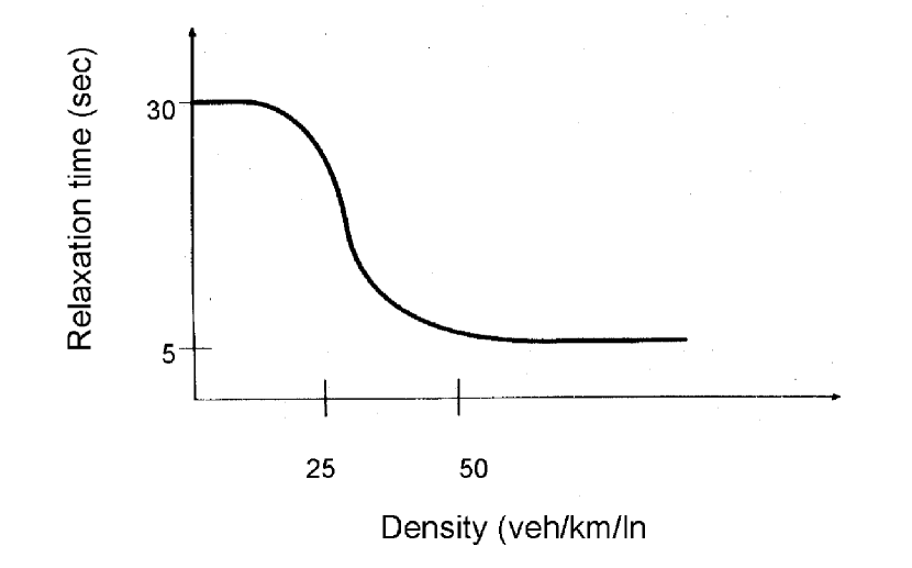
Figure 1: Dependence of the relaxation time $\tilde{T}$ on the vehicle density per lane. Taken from Kühne and Michalopoulos (1997, available online at http://www.tfhrc.gov/its/tft/tft.htm).

However, these values have to be interpreted with care and cannot be translated directly to our model context. To see this, we note that the relaxation time $\tilde{T}$ is determined for the ansatz $v(t,x)=u(\rho(t+\tilde{T},x+\Delta x))$, i.e. after the relaxation time $\tilde{T}$ the driver has fully adjusted to the equilibrium velocity $u$. Here, according to Eqs. (15) and (16), the equilibrium velocity in general will never be reached exactly. Instead, if we require, that $|v(t)-u(t)|<|v(0)-u(0)|/1000$, we find that $t>6.908~{}T\approx\tilde{T}$. I hence seems reasonable to set

$$\tilde{T}\approx 5~{}..~{}10~{}T.$$ (25)

Taking average values $\tau=0.75~{}\mbox{s}$ and $\tilde{T}=7.5~{}T$, we indeed find that $T-\tau<0$ for about $\rho>50$ [1/km/lane]. It was also pointed out in Kühne and Michalopoulos (1997, available online at http://www.tfhrc.gov/its/tft/tft.htm) that for large densities the relaxation time $\tilde{T}$ increases, which means that $T-\tau>0$ for $\rho\approx\rho_{m}$.

One could try to repeat the derivation leading to Eq. (23) for a general relaxation time $T=T(\rho,v)$. Note, that the above derivation is only valid for a constant relaxation time. Moreover, it involves only the leading term of a Taylor series expansion. We therefore decided to generalize the velocity equation of the ARG model in the following way

$$\frac{\partial v}{\partial t}+(v+\rho u^{\prime}(\rho))\frac{\partial v}{\partial x}=\beta(\rho,v)(u(\rho)-v).$$ (26)

Note that we do not require $v\leq u$ as Greenberg Greenberg (2001). From the experimental data and the argument put forward before (note that the sign of $\beta$ determines whether the traffic flow is linearly stable or not) we require

$$\beta(\rho,v)<0{\rm~{}for~{}}0<\rho_{1}<\rho<\rho_{2}<\rho_{m},v=u(\rho),$$ (27)

$$\lim_{\rho\to 0,\rho_{m}}\beta(\rho,v)>0,\hskip 56.9055pt$$ (28)

$$\lim_{v\to 0,u_{m}=u(0)}\beta(\rho,v)>0.\hskip 56.9055pt$$ (29)

Throughout this paper we use a functional form

$$\beta(\rho,v)=\left\{\begin{array}[]{ll}\frac{a_{c}}{u-v},&\mbox{if~{}}\tilde{\beta}(\rho,v)(u-v)-a_{c}\geq 0,\\ \frac{d_{c}}{u-v},&\mbox{if~{}}\tilde{\beta}(\rho,v)(u-v)-d_{c}\leq 0,\\ \tilde{\beta}(\rho,v),&\mbox{else},\end{array}\right.$$ (30)

where the function $\tilde{\beta}(\rho,v)$ is defined as

$$\tilde{\beta}=\frac{1}{\hat{T}}\Big{(}1+\alpha\frac{|u-v|}{u_{m}}+\frac{1}{\rho_{1}\rho_{2}}(-(\rho_{1}+\rho_{2})\rho+\rho^{2})\Big{)}.$$ (31)

For the choice of the velocity-density relation of Cremer Cremer, M. (1979)

$$u(\rho)=u_{m}\Big{(}1-\Big{(}\frac{\rho}{\rho_{m}}\Big{)}^{n_{1}}\Big{)}^{n_{2}}$$ (32)

and the parameters $\rho_{m}=300$ [1/km], $u_{m}=140$ km/h, $n_{1}=0.35$, $n_{2}=1$ (note that with these parameters, the equilibrium velocity of Cremer (32) fulfills the conditions (3) and (4)), $\hat{T}=1$ s, $\alpha=12$, $\rho_{1}=70$ [1/km] and $\rho_{2}=270$ [1/km] the function $\tilde{\beta}(\rho,v)$ already fulfills all requirements (27)-(29). However, due to mechanical restrictions, the maximum acceleration $a_{c}$ and deceleration $d_{c}$ give stronger limitations, i.e.

$$\frac{dv}{dt}\leq a_{c}\mbox{~{}and~{}}\frac{dv}{dt}\geq d_{c}$$ (33)

with typical values $a_{c}=2~{}{\rm m/s^{2}}$ and $d_{c}=-5~{}{\rm m/s^{2}}$. Since the resulting system is not strictly hyperbolic for equality in Eq. (33), which is problematic for a numerical solution, we prescribe the limitations on

$$\frac{d(v-u)}{dt}\leq a_{c}\mbox{~{}and~{}}\frac{d(v-u)}{dt}\geq d_{c},$$ (34)

which then leads to the functional form (30). We plot the function $\beta(\rho,v)$ for the mentioned parameter values in Fig. 2.

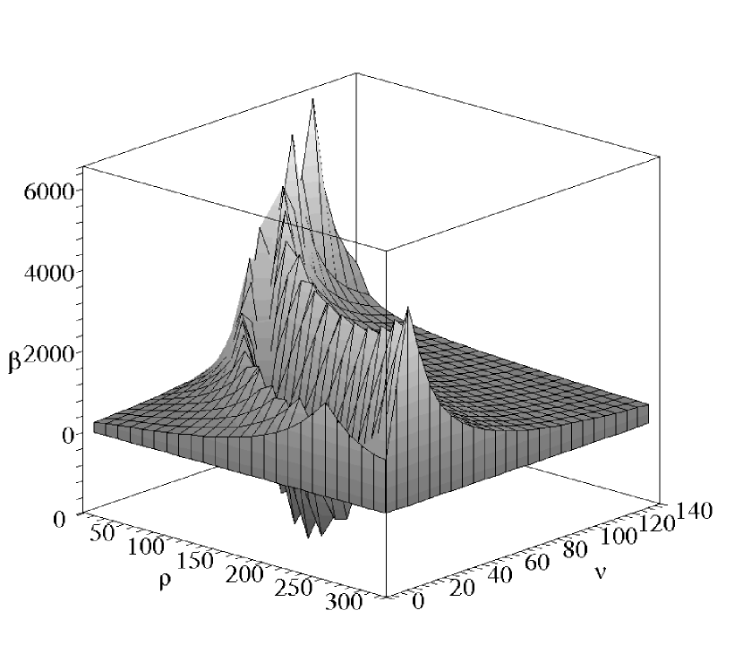
Figure 2: Function $\beta(\rho,v)$ defined in Eq. (30). We used units [$\rho$] = 1/km and [v]=km/h and [$\beta$] = 1/h.

We stress that the above functions describe reality only qualitatively. For realistic simulations of traffic flow, experimental data are required to determine $\beta(\rho,v)$.

In the new model, traffic flow is described by the following system of balance laws

$$\frac{\partial\rho}{\partial t}+\frac{\partial(\rho v)}{\partial x} = 0,$$ (35)

$$\frac{\partial(\rho(v-u(\rho))}{\partial t}+\frac{\partial(\rho v(v-u(\rho)))}{\partial x} = \beta\rho(u-v),$$ (36)

or equivalently for smooth solutions by Eqs. (5) and (26). As the corresponding system of the ARG model, the new system is strictly hyperbolic for $0<\rho\leq\rho_{m}$.

III The numerical implementation

Writing traffic flow as a system of balance laws in Eqs. (35) and (36) is very adequate for numerical purposes, as it allows the application of well-established hydrodynamic methods for the numerical solution. We use a high-resolution shock-capturing scheme with approximate Riemann solver for the numerical solution (see e.g. LeVeque (1992)).

We rewrite Eqs. (35) and (36) in the form

$$\frac{\partial U}{\partial t}+\frac{\partial F(U)}{\partial x}=S(U),$$ (37)

where

$$U = \begin{pmatrix}\rho\cr\rho(v-u)\end{pmatrix}=\begin{pmatrix}U_{1}\cr U_{2}\end{pmatrix},$$ (38)

$$F(U) = \begin{pmatrix}\rho v\cr\rho v(v-u)\end{pmatrix}=\begin{pmatrix}U_{2}+U_{1}u(U_{1})\cr\frac{U_{2}^{2}}{U_{1}}+U_{2}u(U_{1})\end{pmatrix},$$ (39)

$$S(U) = \begin{pmatrix}0\cr\beta\rho(u-v)\end{pmatrix}.$$ (40)

We use the second-order reconstruction scheme of van Leer van Leer (1977) to reconstruct quantities at cell interfaces. At cell $i$ with cell center at the location $x_{i}=x_{0}+i\Delta x$ the update in time from $t^{n}$ to $t^{n+1}$ is performed according to an conservative algorithm

$$U_{i}^{n+1}=U_{i}^{n}-\frac{\Delta t}{\Delta x}(\hat{F}_{i+\frac{1}{2}}-\hat{F}_{i-\frac{1}{2}})+\Delta tS_{i},$$ (41)

where $U_{i}^{n}=U(x_{i},t^{n})$ and $\Delta t=t^{n+1}-t^{n}$. To obtain a higher order of convergence, we use the third order scheme of Shu and Osher Shu and Osher (1989). The numerical fluxes $\hat{F}$ are determined according to the flux-formula of Marquina Donat and Marquina (1996), which reads

$$\hat{F}=\frac{1}{2}(F^{R}+F^{L}-\Delta q).$$ (42)

Here, the superscripts $R$ and $L$ denote the reconstructed values on the right and left of a cell interface. The numerical viscosity term takes the form

$$\Delta q=\mathbf{R}^{R}|\mathbf{\Lambda}|_{\max}\mathbf{L}^{R}U^{R}-\mathbf{R}^{L}|\mathbf{\Lambda}|_{max}\mathbf{L}^{L}U^{L}.$$ (43)

The matrix $|\mathbf{\Lambda}|_{\max}$ involves the characteristic speeds,

$$|\mathbf{\Lambda}|_{\max}=\begin{pmatrix}\max(|\lambda_{1}^{R}|,|\lambda_{1}^{L}|)&0\cr 0&\max(|\lambda_{2}^{R}|,|\lambda_{2}^{L}|)\end{pmatrix},$$ (44)

where the characteristic speeds read explicitly

$$\lambda_{1} = v+\rho u^{\prime},$$ (45)

$$\lambda_{2} = v.$$ (46)

$\mathbf{R}$ and $\mathbf{L}$ are the matrices of the right and left eigenvectors of the matrix

$$\frac{\partial F}{\partial U}=\begin{pmatrix}u+\rho u^{\prime}&1\cr-(v-u)^{2}+\rho(v-u)u^{\prime}&2v-u\end{pmatrix}.$$ (47)

Explicitly,

$$\mathbf{R} = \begin{pmatrix}1&1\cr u-v&v-u-\rho u^{\prime}\end{pmatrix},$$ (48)

$$\mathbf{L} = \frac{1}{\rho u^{\prime}}\begin{pmatrix}u-v+\rho u^{\prime}&1\cr v-u&-1\end{pmatrix}.$$ (49)

IV Code tests

We checked, that our numerical algorithm is convergent. Moreover, the density equation (35) is a strict conservation law. Prescribing periodic boundary conditions as in Sec. V, the total number of cars included in the numerical domain $\Omega$ should therefore be constant, i.e.

$$\int_{\Omega}\rho~{}dx=\mbox{const}.$$ (50)

We checked, that our numerical code fulfills Eq. (50) up to machine precision (see also the corresponding results for a network simulation based on the Lighthill-Whitham theory in Siebel and Mauser (2005)).

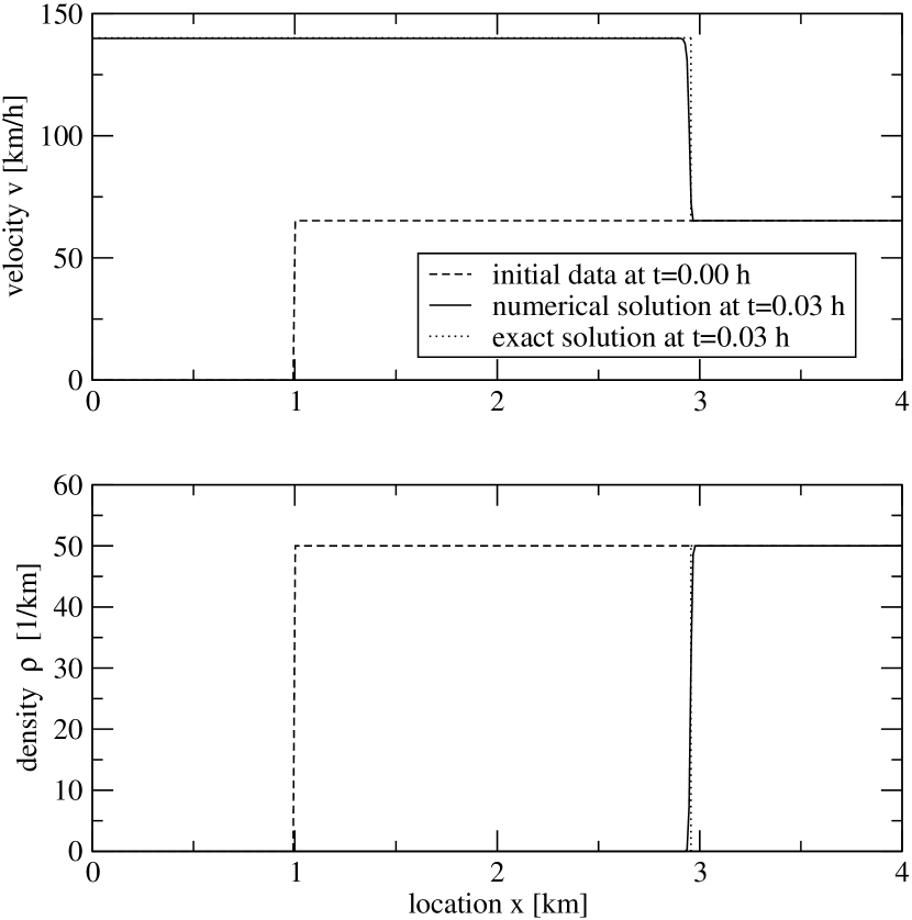
Figure 3: Numerical solution for a Riemann problem of Aw and Rascle Aw and Rascle (2000). The numerical solution at time t=0.03 h (solid line) for the initial data (dashed line) reproduces the exact solution (dotted line).

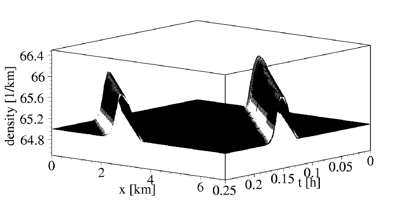
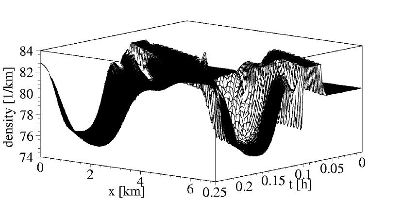
Figure 4: Time evolution of the density for stable and instable initial data. We prescribe an equilibrium density $\rho_{0}=65$ [1/km] and $\rho_{0}=80$ [1/km] respectively, and on top a sinusoidal density perturbation. For the instable data, the initial perturbation located at $x=2.5$ [km] is amplified and finally two clusters form.

Finally, Aw and Rascle presented in their paper the exact solution of a Riemann problem, for which old two-equation models fail to describe the correct behavior (see Aw and Rascle (2000), Fig. 5.4). This Riemann problem consists of the following initial data

$$\rho = \left\{\begin{array}[]{ll}0,&\mbox{if~{}}x<1\mbox{~{}km},\\ \rho_{+},&\mbox{if~{}}x\geq 1\mbox{~{}km},\end{array}\right.$$ (53)

$$v = \left\{\begin{array}[]{ll}0,&\mbox{if~{}}x<1\mbox{~{}km},\\ v_{+},&\mbox{if~{}}x\geq 1\mbox{~{}km}.\end{array}\right.$$ (56)

The exact solution to the homogeneous system consists of the constant state on the right $(\rho_{+},v_{+})$ moving to the right with velocity $v_{+}$, leaving behind vacuum. If we chose $v_{+}=u(\rho_{+})$, this exact solution will carry over to our inhomogeneous system. Fig. 3 displays our numerical solution for a choice $\rho_{+}=50$ [1/km]. For numerical reasons, we prescribe a density $\rho=10^{-6}$ [1/km] for $x<1$ km. Note, that our numerical algorithm resolves the steep gradient within only a few grid cells, at the same time reproducing the correct velocity at which the constant state moves to the right. Moreover, the velocity relaxes to the equilibrium velocity behind the constant state $(\rho_{+},v_{+})$.

V Results on the fundamental diagram

For the results presented in this section we restrict us to a 7 km long section of a (two-lane) highway with periodic boundary conditions. On this section of the highway, we start our simulations with constant equilibrium data $\rho=\rho_{0}$, $v=u(\rho_{0})$ and in addition between kilometers 2 and 3 a sinusoidal density perturbation

$$\Delta\rho=\sin(\pi x){\ \rm~{}for~{}2~{}<~{}}x{\rm~{}<~{}3~{}km}.$$ (57)

For all presented numerical results we used a resolution of 50 m. Fig. 4 shows the evolution of these data for parameters $\rho_{0}=65$ [1/km] and $\rho_{0}=80$ [1/km]. Whereas the amplitude of the perturbation is gradually damped with time for the stable initial data $\rho_{0}=65$ [1/km], the amplitude of the perturbation increases for the instable initial data $\rho_{0}=80$ [1/km]. Moreover, the perturbation travels with a larger velocity downstream in the first case. For the unstable situation, two clusters are forming. We plot the corresponding time evolutions of the velocity in Fig. 5.

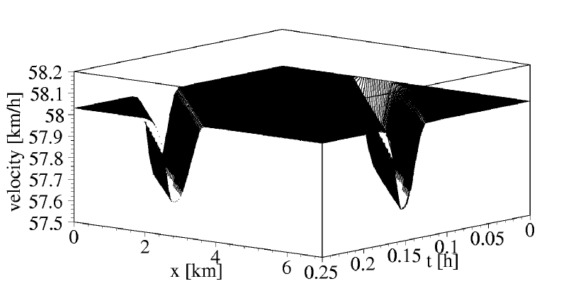
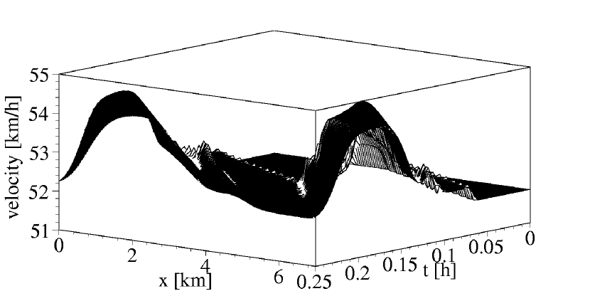
Figure 5: Time evolution of the velocity for stable ($\rho_{0}=65$ [1/km]) and instable initial data ($\rho_{0}=80$ [1/km]) with initial density perturbation.

To obtain a more general picture we varied the initial density in the entire density regime and analyzed the resulting flow-density-relation as a function of time. More precisely, we used initial values for the equilibrium data $\rho_{0}=2,4,....,298$ and read off the resulting values for the density $\rho$ and the flux function $\rho v$ at 5 equidistantly distributed cross sections of the highway. Fig. 6 shows the results for evolution times $t=0.00$ h (initial data), $t=0.05$ h, $t=0.10$ h, $t=0.15$ h, $t=0.20$ h and $t=0.25$ h.

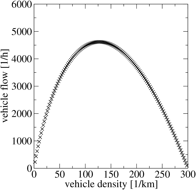
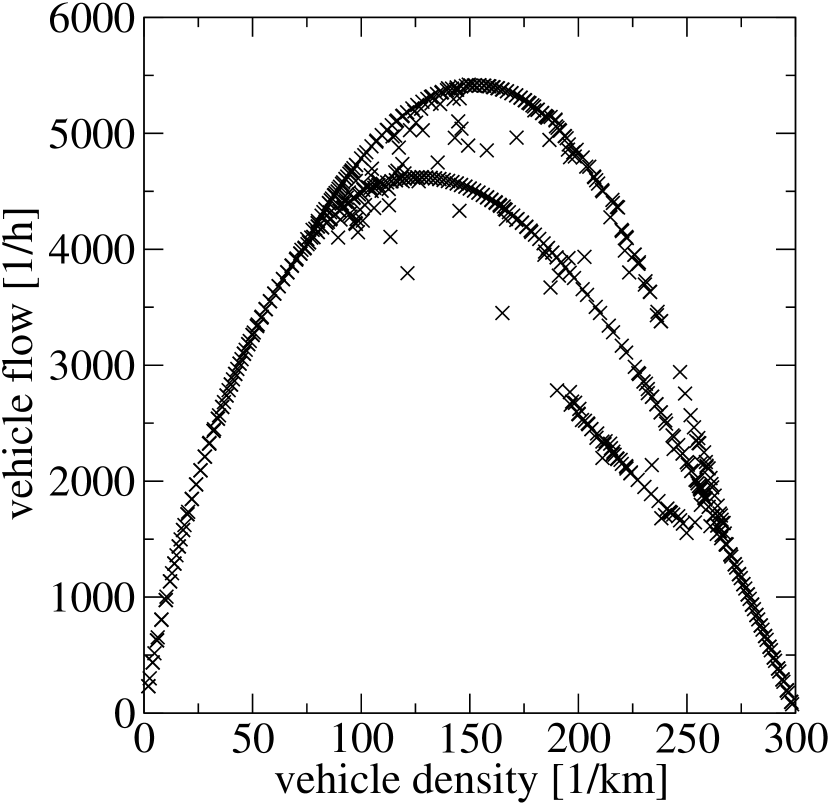
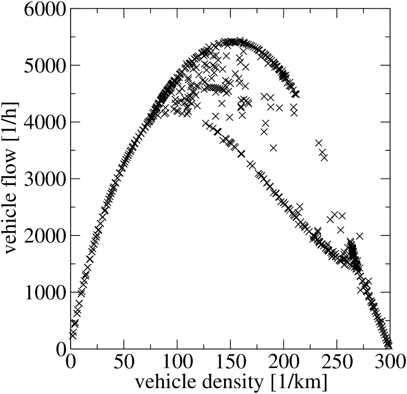
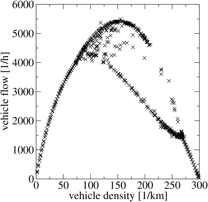
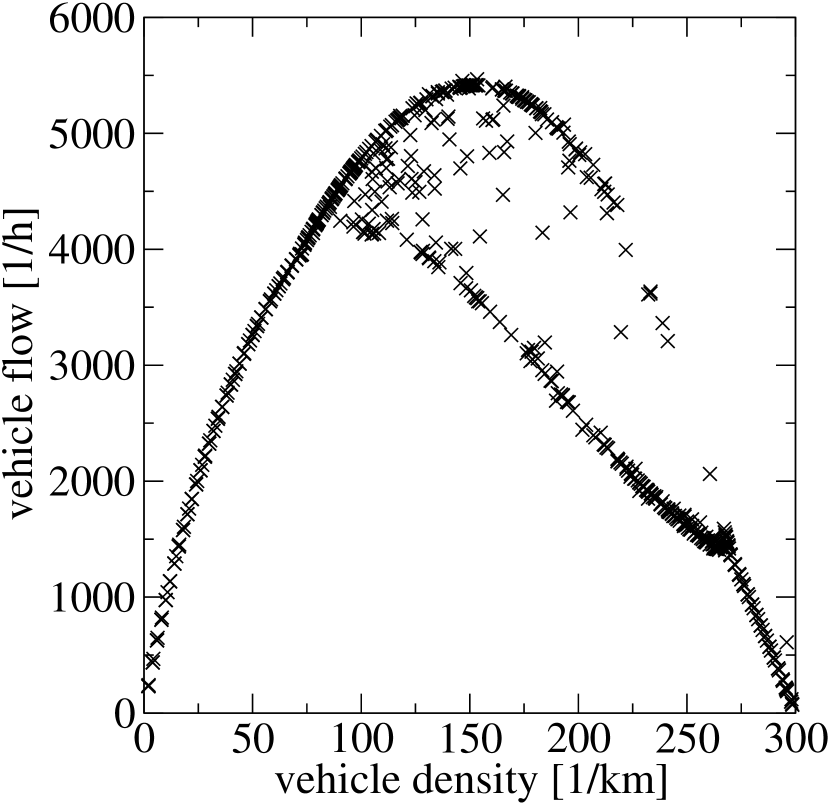
Figure 6: Fundamental diagram for the initial data (t = 0.00 h) (first row on the left), for t = 0.05 h (first row on the right), for t = 0.10 h (second row on the left), for t = 0.15 h (second row on the right), for t = 0.20 h (third row on the left) and for t = 0.25 h (third row on the right). At intermediate densities, our traffic model is linearly unstable, the representative points in the fundamental diagram are shifted towards two branches, which gives the visual impression of an inverted $\lambda$.

For the initial data, the flow-density curve corresponds closely to the equilibrium flow density, the initial perturbation (57) being negligible for the visual output. After an evolution time $t=0.05$ h, the equilibrium flow-density-curve is still visible, but in the unstable regime for densities $70<\rho<270$ [1/km] two new flow-density-curves start to appear. In the evolution further in time, the equilibrium density curve vanishes. Instead the two new branches produce an inverse-$\lambda$ shape.

VI Conclusion and Outlook

We generalized the traffic model of Aw, Rascle and Greenberg by prescribing a more general source term to the velocity equation and developed a new numerical code to solve the resulting system of balance laws. In total our (numerical) results show:

• The new model can explain the large variance of the measured values of the fundamental diagram in the congested regime, which correspond to fluctuations between two branches in the unstable density regime. Moreover, due to the stability properties, the model predicts oscillations in the relative velocity of cars in the congested regime, as they are found in experimental data. At the same time, it reproduces the small variance of velocities for free traffic flow and can explain the appearance of wide traffic jams.

• Macroscopic traffic models have often used an equilibrium velocity $u(\rho)$, for which $\frac{d(\rho u(\rho))}{d\rho^{2}}>0$ in the congested regime, in order to account for the values of traffic flow at the maximum (the tip of the inverted $\lambda$). According to our study, this is not necessary, as the high values for the fluxes can be explained with overcritical solutions and an equilibrium velocity function with $\frac{d(\rho u(\rho))}{d\rho^{2}}<0$ everywhere.

The new model, which is a deterministic and effective one-lane model, has the capacity of reproducing many features observed in traffic dynamics. In the presented work, the form of the function $\beta$ in Fig. 2 was motivated by a physical argument, but the quantitative details were determined rather ad hoc. However, we found that the fundamental diagram in the unstable region (e.g. the tip of the inverted $\lambda$) depends on the particular form of $\beta$. Hence one should try to determine the function $\beta$ from experimental data of the fundamental diagram. In our opinion, the presented algorithm is adequate for the use in network simulations of traffic flow.

References

- Daganzo (1995) C. Daganzo, Transportation Research B 29, 277 (1995).
- Zhang (1998) H. M. Zhang, Transportation Research B 32, 485 (1998).
- Jiang et al. (2002) R. Jiang, Q.-S. Wu, and Q.-S. Zhu, Transportation Research B 36, 405 (2002).
- Aw and Rascle (2000) A. Aw and M. Rascle, SIAM Journal of Applied Mathematics 60, 916 (2000).
- Greenberg (2001) J. Greenberg, SIAM Journal of Applied Mathematics 62, 729 (2001).
- Lighthill and Whitham (1955) M. Lighthill and G. Whitham, Proceedings of the Royal Society A 229, 317 (1955).
- Richards (1956) P. Richards, Operations Research 4, 42 (1956).
- Whitham, G.B. (1974) Whitham, G.B., Linear and Nonlinear Waves (John Wiley, New York, 1974).
- Schönhof and Helbing (2004) M. Schönhof and D. Helbing, cond-mat/0408138 (2004).
- Helbing (2001) D. Helbing, Reviews of Modern Physics 73, 1067 (2001).
- Greenberg et al. (2003) J. Greenberg, A. Klar, and M. Rascle, SIAM Journal of Applied Mathematics 63, 818 (2003).
- Aw et al. (2002) A. Aw, A. Klar, T. Materne, and M. Rascle, SIAM Journal of Applied Mathematics 63, 259 (2002).
- Bando et al. (1995) M. Bando, K. Hasebe, A. Nakayama, A. Shibata, and Y. Sugiyama, Phys. Rev. E 51, 1035 (1995).
- Treiber et al. (1999) M. Treiber, A. Hennecke, and D. Helbing, Phys. Rev. E 59, 239 (1999).
- Nelson (2000) P. Nelson, Phys. Rev. E 61, R6052 (2000).
- Kühne and Michalopoulos (1997, available online at http://www.tfhrc.gov/its/tft/tft.htm) R. Kühne and P. Michalopoulos, in Transportation Research Board special report 165, 5 (1997, available online at http://www.tfhrc.gov/its/tft/tft.htm).
- Cremer, M. (1979) Cremer, M., Der Verkehrsfluß auf Schnellstraßen (Traffic Flow on Freeways) (Springer, 1979).
- LeVeque (1992) R. J. LeVeque, Numerical methods for conservation laws (Birkhäuser, Basel, 1992).
- van Leer (1977) B. J. van Leer, J. Comp. Phys. 23, 276 (1977).
- Shu and Osher (1989) C.-W. Shu and S. Osher, J. Comp. Phys. 83, 32 (1989).
- Donat and Marquina (1996) R. Donat and A. Marquina, J. Comp. Phys. 146, 42 (1996).
- Siebel and Mauser (2005) F. Siebel and W. Mauser, Mathematical and Computer Modelling of Dynamical Systems, in press (2005).