Self-gravitating Brownian systems and bacterial populations with two or more types of particles.

Abstract

We study the thermodynamical properties of a self-gravitating gas with two or more types of particles. Using the method of linear series of equilibria, we determine the structure and stability of statistical equilibrium states in both microcanonical and canonical ensembles. We show how the critical temperature (Jeans instability) and the critical energy (Antonov instability) depend on the relative mass of the particles and on the dimension of space. We then study the dynamical evolution of a multi-components gas of self-gravitating Brownian particles in the canonical ensemble. Self-similar solutions describing the collapse below the critical temperature are obtained analytically. We find particle segregation, with the scaling profile of the slowest collapsing particles decaying with a non universal exponent that we compute perturbatively in different limits. These results are compared with numerical simulations of the two-species Smoluchowski-Poisson system. Our model of self-attracting Brownian particles also describes the chemotactic aggregation of a multi-species system of bacteria in biology.

1 Introduction

In previous papers of this series [1]-[8], we have introduced a model of self-gravitating Brownian particles and we studied its equilibrium and collapse properties in the framework of thermodynamics. In this model, the motion of the particles is described by $N$ coupled stochastic equations (one for each particle) involving a friction and a random force in addition to self-gravity. The friction and the random force mimic the influence of a thermal bath of non-gravitational origin imposing the temperature. The temperature of the bath measures the strength of the stochastic force. The self-gravitating Brownian gas model has a conceptual interest in physics because it represents the canonical counterpart of a Hamiltonian system of stars in Newtonian interaction. Therefore, it can be used to test dynamically the inequivalence of statistical ensembles which is generic for systems with long-range interactions. Although most astrophysical systems are described by the Newton equations (without dissipation), the self-gravitating Brownian gas model could find applications for the transport of dust particles in the solar nebula and the formation of planetesimals by gravitational instability [9]. In this situation, the particles experience a drag force due to the friction with the gas and a stochastic force due to turbulence. Furthermore, self-gravity must be taken into account when the particles have grown sufficiently by sticking processes and start to feel their mutual attraction. This would be just a first step because other ingredients are required to improve the description of planetesimal formation. It has also been shown in [10] that the process of violent relaxation for collisionless stellar systems exhibits similarities with the dynamics of a self-gravitating Brownian gas. In particular, the coarse-grained distribution function $\overline{f}({\bf r},{\bf v},t)$ satisfies a generalized Fokker-Planck equation, involving an effective diffusion and an effective friction taking into account the peculiarities of the collisionless evolution.

Our model of self-gravitating Brownian particles has also interest for systems that are not necessarily related to astrophysics. For example, in the physics of ultra cold gases, it has been shown recently that, using a clever configuration of lasers beams, it is possible to create an attractive $1/r$ interaction between atoms [11]. This leads to the fascinating possibility of reproducing gravitational instabilities in the laboratory. In particular, it is argued in [12] that it should be possible to observe the “isothermal collapse” [13, 14] of a Fermi gas cloud in thermal equilibrium with a bosonic “reservoir”. Since the system is essentially dissipative a canonical description (fixed $T$) is required and a plausible dynamical description of the system would be formed by the Fokker-Planck equation coupled to the gravitational Poisson equation. In that case, the quantum nature of the particles (fermions) is important, and generalized Fokker-Planck equations, including the Pauli exclusion principle, must be considered as in [6]. On the other hand, as discussed in our previous papers, the collapse of the self-gravitating Brownian gas is analogous to the chemotactic aggregation of bacterial populations in biology. In particular, the Smoluchowski-Poisson system which describes self-gravitating Brownian particles in a strong friction limit is isomorphic to a simplified version of the Keller-Segel model [15] in biology, obtained in the limit of large diffusivity of the chemical [16]. The Keller-Segel model is a standard model in mathematical biology [17]. Due to this analogy, the results of [1]-[8] have direct application for the chemotactic aggregation of bacterial populations.

For all these reasons, and also in its own right, the study of the self-gravitating Brownian gas model [1] is clearly of interest in physics. So far, most works have focused on the case of a single species of particles. In this paper, we extend these approaches to the case of a multi-components system, with particular attention devoted to the two-species model. In Sec. 2, we present the basic equations describing a multi-components self-gravitating Hamiltonian and Brownian system and show the analogies of the latter with a multi-components chemotactic system. We use a mean-field approach which is exact in a suitable thermodynamic limit $N_{\alpha}\rightarrow+\infty$, keeping $\eta_{\alpha}=\beta Gm^{2}_{\alpha}N_{\alpha}/R^{d-2}$ constant for each species $\alpha$ (see Appendix A). In Sec. 3, we discuss the statistical equilibrium states of a two-components self-gravitating system in both microcanonical and canonical ensembles. Therefore, our static study applies both to ordinary stellar systems (galaxies, globular clusters,…) described in the microcanonical ensemble and Brownian systems (or bacteria) described in the canonical ensemble. We obtain the equilibrium density profiles and analyze their thermodynamical stability by drawing the linear series of equilibria (caloric curves) and using the turning point argument [18]. We show how the critical temperature (Jeans instability [13]) and the critical energy (Antonov instability [19, 20]) depend on the parameters $\mu=m_{1}/m_{2}$ and $\chi=M_{1}/M_{2}$ where $m_{\alpha}$ is the individual mass of the particles and $M_{\alpha}=N_{\alpha}m_{\alpha}$ the total mass of species $\alpha$. In the microcanonical ensemble, we find that the gravothermal catastrophe is advanced, i.e. it occurs sooner with respect to the single-species case. In the canonical ensemble, the isothermal collapse is advanced if we add heavy particles in the system and delayed if we add lighter particles (keeping the total mass fixed). Exact analytical expressions of the critical temperature of collapse are given in dimension $d=2$. An approximate expression is obtained for $d>2$ by using the Jeans swindle (see Appendix B). Our static study (Sec. 3) completes previous investigations by Taff et al. [21] and De Vega & Siebert [22] in $d=3$ and Yawn & Miller [23] in $d=1$. In Sec. 4, we consider for the first time the dynamics of the two-species self-gravitating Brownian gas in a strong friction limit described by the Smoluchowski-Poisson system. We study the collapse below $T_{c}$ by looking for self-similar solutions. Depending on the values of $\mu$ and $\zeta=\xi_{1}/\xi_{2}$, where $\xi_{\alpha}$ are the friction coefficients, we show that the collapse of one species of particles dominates the other. The invariant profile of the dominant species scales as $\rho\sim r^{-2}$ as for the one-component gas [1]. The collapse of the other particles is slaved to the collapse of the dominant species. This decouples the equations of motion and reduces the problem to the study of a single new dynamical equation. We show that this equation possesses self-similar solutions and that the scaling profile scales as $\rho\sim r^{-\alpha}$ where $\alpha$ is a non-trivial exponent depending on $\mu$, $\zeta$ and $d$, which leads to particle segregation. We determine this scaling exponent perturbatively in a large dimension limit $d\rightarrow+\infty$ on the one hand and for a weak asymmetry $\mu\rightarrow 1$ and $\zeta\rightarrow 1$ on the other hand. We also consider the limits $\mu\rightarrow 0,+\infty$ or $\zeta\rightarrow 0,+\infty$. These perturbative analytical results are compared with the exact results obtained numerically.

2 Analogy between self-gravitating Brownian particles and bacterial populations

2.1 Self-gravitating Hamiltonian systems with different species of particles

Let us consider a Hamiltonian system of $X$ species of particles with mass $m_{1},{...},m_{X}$ in a space of dimension $d$. Throughout the paper, the particles of species $1$ are labeled from $i=1$ to $g_{1}N$, the particles of species 2 from $(g_{1}N+1)$ to $g_{2}N$, and so on up to species $X$. The Latin letters $i$ will index the $N$ particles and the Greek letters $\alpha$ will index the $X$ species. The particles interact via a long-range potential $U(\textbf{r}_{1},{...},\textbf{r}_{N})=\sum_{i<j}m_{i}m_{j}u(\textbf{r}_{i}-\textbf{r}_{j})$. In this paper, $u(\textbf{r}_{i}-\textbf{r}_{j})=-G/[{(d-2)|\textbf{r}_{i}-\textbf{r}_{j}|^{(d-2)}}]$ denotes the gravitational potential of interaction in $d$ dimensions. This Hamiltonian system is completely defined by the equations of motion

$$\begin{array}[]{rcl}\displaystyle\frac{d\textbf{r}_{i}}{dt}&=&\textbf{v}_{i}\,,\vspace{6pt}\\ \displaystyle\frac{d\textbf{v}_{i}}{dt}&=&\displaystyle-\frac{1}{m_{i}}\nabla_{i}U(\textbf{r}_{1},{...},\textbf{r}_{N}).\end{array}$$ (3)

In kinetic theory, the collisionless evolution of this system is governed by the Vlasov-Poisson system, which is valid for sufficiently “short” times. In fact, this regime can be extremely long in practice since the relaxation time (Chandrasekhar’s time) increases almost linearly with the number of particles. The collisional regime is usually described by the Landau-Poisson system which governs the evolution of the distribution function $f({\bf r},{\bf v},t)$ toward statistical equilibrium. For a multi-species system in $d=3$, the Landau equation reads

$$\frac{\partial f_{\alpha}}{\partial t}+\textbf{v}\cdot\frac{\partial f_{\alpha}}{\partial\textbf{r}}+\textbf{F}\cdot\frac{\partial f_{\alpha}}{\partial\textbf{v}}=\frac{\partial}{\partial v^{\mu}}\sum_{\gamma=1}^{X}\int K^{\mu\nu}\left(m_{\gamma}f^{\prime}_{\gamma}\frac{\partial f_{\alpha}}{\partial v^{\nu}}-m_{\alpha}f_{\alpha}\frac{\partial f^{\prime}_{\gamma}}{\partial v^{\prime\nu}}\right)\,d{\bf v}^{\prime},$$

$$K^{\mu\nu}=2\pi G^{2}\frac{1}{u}\ln\Lambda\left(\delta^{\mu\nu}-\frac{u^{\mu}u^{\nu}}{u^{2}}\right),\qquad\qquad\qquad$$ (4)

where $\textbf{u}=\textbf{v}-\textbf{v}^{\prime}$ is the relative velocity of the particles involved in an encounter, $\ln\Lambda=\int_{0}^{+\infty}\,dk/k$ is the Coulomb factor (which must be appropriately regularized) and $\textbf{F}=-\nabla\Phi$ is the gravitational force per unit of mass. We have also set $f_{\alpha}^{\prime}=f_{\alpha}({\bf r},{\bf v}^{\prime},t)$ assuming that the encounters can be treated as local (see [24] for a critical discussion of this approximation). The gravitational potential $\Phi(\textbf{r},t)$ is determined by the Poisson equation

$$\Delta\Phi=S_{d}G\rho,$$ (5)

with the total density $\rho=\sum_{\alpha=1}^{X}\rho_{\alpha}$, where $\rho_{\alpha}({\bf r},t)=\int f_{\alpha}({\bf r},{\bf v},t)\,d{\bf v}$ is the spatial density of species $\alpha$ and $f_{\alpha}({\bf r},{\bf v},t)$ is their distribution function ($f_{\alpha}({\bf r},{\bf v},t)\,d{\bf r}\,d{\bf v}$ gives the total mass of particles of species $\alpha$ with position in (${\bf r}\,;\,{\bf r}+d{\bf r}$) and velocity in (${\bf v}\,;\,{\bf v}+d{\bf v}$) at time $t$). The total distribution function is $f=\sum_{\alpha=1}^{X}f_{\alpha}$.

The Landau-Poisson system conserves the total mass

$$M_{\alpha}=\int\rho_{\alpha}\,d{\bf r}=N_{\alpha}m_{\alpha},$$ (6)

of each species and the total energy

$$E=\frac{1}{2}\int fv^{2}\,d{\bf r}\,d{\bf v}+\frac{1}{2}\int\rho\Phi\,d{\bf r}=K+W,$$ (7)

where $K$ is the kinetic energy and $W$ is the potential energy. Furthermore, the Landau-Poisson system satisfies a H-theorem $\dot{S}\geq 0$ for the multi-components Boltzmann entropy

$$S=-k_{B}\sum_{\alpha=1}^{X}\int\frac{f_{\alpha}}{m_{\alpha}}\ln\left(\frac{f_{\alpha}}{m_{\alpha}}\right)\,d{\bf r}\,d{\bf v}.$$ (8)

At equilibrium, $\dot{S}=0$ implying that the current in the R.H.S of Eq. (2.1) must vanish. The advective term in the L.H.S of this equation must also vanish, independently. These two conditions imply that the only stationary solution of the Landau equation (2.1) is the Maxwell-Boltzmann distribution

$$f_{\alpha}(\textbf{r},\textbf{v})=A_{\alpha}\left(\frac{m_{\alpha}\beta}{2\pi}\right)^{d/2}e^{-\beta m_{\alpha}\left[\frac{v^{2}}{2}+\Phi(\textbf{r})\right]},$$ (9)

where the inverse temperature $\beta=1/k_{B}T$ appears as an integration constant. Note that the advective term (Vlasov) is canceled out by any distribution function $f_{\alpha}=f_{\alpha}(\epsilon)$ depending on the particle energy $\epsilon=\frac{v^{2}}{2}+\Phi({\bf r})$ alone. The cancellation of the collision term singles out the Boltzmann distribution among this infinite class of distributions. The Maxwell-Boltzmann distribution Eq. (9) represents the statistical equilibrium state of the system in a mean-field approximation. It can be obtained alternatively by maximizing the entropy (8) at fixed energy and particle number (for each species). The condition of thermodynamical stability in the microcanonical ensemble (maximum of $S$ at fixed $E$, $N_{\alpha}$) is equivalent to the linear dynamical stability with respect to the Landau-Poisson system [25].

According to the theorem of equipartition of energy (which remains valid here), the r.m.s. velocity of species $\alpha$ decreases with mass such that

$$\langle v^{2}\rangle_{\alpha}=\frac{\int e^{-\beta m_{\alpha}\frac{v^{2}}{2}}v^{2}d{\bf v}}{\int e^{-\beta m_{\alpha}\frac{v^{2}}{2}}d{\bf v}}=d\frac{k_{B}T}{m_{\alpha}}.$$ (10)

Therefore, heavy particles have less velocity dispersion to resist gravitational attraction and will preferentially orbit in the inner region of the system. This leads to mass segregation, but of a very different nature from the dynamical segregation that we study in Section 4. Defining the pressure by $p=\frac{1}{d}\int fv^{2}d{\bf v}$, we get from Eq. (10) the local equation of state

$$p=\sum_{\alpha=1}^{X}\frac{\rho_{\alpha}}{m_{\alpha}}k_{B}T.$$ (11)

The local mass density $\rho_{\alpha}$ of each species is obtained directly from the integration of Eq. (9) over the velocities yielding

$$\rho_{\alpha}(\textbf{r})=A_{\alpha}e^{-\beta m_{\alpha}\Phi(\textbf{r})}.$$ (12)

The gravitational field $\Phi({\bf r})$ is obtained self-consistently by substituting Eq. (12) in the Poisson equation (5) and solving the resulting differential equation.

2.2 Self-gravitating Brownian particles with different species of particles

The Hamiltonian system of stars presented in Sec. 2.1 is associated to the microcanonical ensemble (fixed energy) in statistical mechanics. We shall now introduce a model of particles in Newtonian interaction associated with the canonical ensemble (fixed temperature). Specifically, we consider a system of $N$ self-gravitating Brownian particles belonging to $X$ different species. This is the generalization of the model introduced in [1]. This system is characterized by $N$ coupled stochastic equations

$$\begin{array}[]{rcl}\displaystyle\frac{d\textbf{r}_{i}}{dt}&=&\textbf{v}_{i},\vspace{6pt}\\ \displaystyle\frac{d\textbf{v}_{i}}{dt}&=&\displaystyle-\xi_{i}\textbf{v}_{i}-\frac{1}{m_{i}}\nabla_{i}U(\textbf{r}_{1},{...},\textbf{r}_{N})+\sqrt{2D_{i}}\textbf{R}_{i}(t),\end{array}$$ (15)

where $\xi_{i}$ is the friction coefficient, $D_{i}$ is the diffusion coefficient and $\textbf{R}_{i}(t)$ the stochastic force. In this paper $\textbf{R}_{i}(t)$ is a white-noise satisfying the conditions $\left<\textbf{R}_{i}(t)\right>=0$ and $\left<R_{a,i}(t)R_{b,j}(t^{\prime})\right>=\delta_{ab}\delta_{ij}\delta(t-t^{\prime})$ where $i,j$ refers to the particles and $a,b$ to the space coordinates. The diffusion coefficient and the friction coefficient are related to each other by the Einstein relation (see Appendix A)

$$D_{\alpha}=\frac{\xi_{\alpha}k_{B}T}{m_{\alpha}},$$ (16)

where $T$ is the thermodynamical temperature. Therefore, the temperature measures the strength of the stochastic force.

In the mean-field approximation, the evolution of the system is governed by the multi-components Kramers equation (see Appendix A for details)

$$\frac{\partial f_{\alpha}}{\partial t}+\textbf{v}\cdot\frac{\partial f_{\alpha}}{\partial\textbf{r}}+\textbf{F}\cdot\frac{\partial f_{\alpha}}{\partial\textbf{v}}=\frac{\partial}{\partial\textbf{v}}\cdot\left(D_{\alpha}\frac{\partial f_{\alpha}}{\partial\textbf{v}}+\xi_{\alpha}f_{\alpha}\textbf{v}\right),$$ (17)

which must be coupled consistently with the Poisson equation, using ${\bf F}=-\nabla\Phi$. The Kramers-Poisson system conserves the total mass of each species. Since the system is dissipative, the energy (7) is not conserved and the entropy (8) does not increase monotonically. However, introducing the free energy

$$F[\{f_{\alpha}\}]=E[\{f_{\alpha}\}]-TS[\{f_{\alpha}\}],$$ (18)

the Kramers-Poisson system satisfies a sort of canonical H-theorem $\dot{F}\leq 0$. At equilibrium, $\dot{F}=0$ implying that the diffusion current in Eq. (17) must vanish. The advective term must also vanish. These two conditions lead to the Maxwell-Boltzmann distribution (9) where $1/\beta$ is the temperature of the bath. This distribution represents the statistical equilibrium state of the system in a mean-field approximation. It can be obtained alternatively by minimizing the free energy (18) at fixed particle number (for each species). The condition of thermodynamical stability in the canonical ensemble (minimum of $F$ at fixed $N_{\alpha}$) is equivalent to the linear dynamical stability with respect to the Kramers-Poisson system [25].

In order to simplify the problem further, we consider the strong friction limit and let $\xi_{i}\rightarrow+\infty$ for each particle $i$. This amounts to neglecting the inertia of the particles. Instead of Eq. (15), we obtain a simpler system of coupled stochastic equations

$$\frac{d\textbf{r}_{i}}{dt}=-{\mu_{i}}\nabla_{i}U(\textbf{r}_{1},{...},\textbf{r}_{N})+\sqrt{2D^{\prime}_{i}}\textbf{R}_{i}(t),$$ (19)

where $\mu_{i}=1/m_{i}\xi_{i}$ is the mobility and $D^{\prime}_{i}=D_{i}/\xi_{i}^{2}=k_{B}T/m_{i}\xi_{i}$ is the diffusion coefficient in physical space. The mean-field Fokker-Planck equation obtained in this limit of strong friction is the Smoluchowski equation, which can be written for each species

$$\frac{\partial\rho_{\alpha}}{\partial t}=\frac{1}{\xi_{\alpha}}\nabla\cdot\left(\frac{k_{B}T}{m_{\alpha}}\nabla\rho_{\alpha}+\rho_{\alpha}\nabla\Phi\right).$$ (20)

It has to be solved in conjunction with the Poisson equation (5). The passage from the Kramers to the Smoluchowski equation can be made rigorous by using a Chapman-Enskog expansion (see [26] for details and generalizations). In the $\xi_{\alpha}\rightarrow+\infty$ limit, the distribution function can be written

$$f_{\alpha}(\textbf{r},\textbf{v},t)=\left(\frac{\beta m_{\alpha}}{2\pi}\right)^{d/2}\rho_{\alpha}(\textbf{r},t)e^{-m_{\alpha}\beta\frac{v^{2}}{2}}+O\left(\frac{1}{\xi_{\alpha}}\right),$$ (21)

where $\rho_{\alpha}(\textbf{r},t)$ evolves according to Eq. (20). Using Eqs. (18) and (21), it is possible to express the free energy as a functional of the spatial density of each species in the form

$$F[\{\rho_{\alpha}\}]=\frac{1}{2}\int\rho\Phi\,d{\bf r}+k_{B}T\sum_{\alpha=1}^{X}\int\frac{\rho_{\alpha}}{m_{\alpha}}\ln\left(\frac{\rho_{\alpha}}{m_{\alpha}}\right)\,d{\bf r},$$ (22)

up to an irrelevant additive constant. The Smoluchowski-Poisson system conserves the total mass of each species and decreases the free energy $\dot{F}\leq 0$. At equilibrium, the density is given by Eq. (12). The linearly dynamically stable steady states minimize the free energy $F[\{\rho_{\alpha}\}]$ at fixed mass (for each species) [25].

The Kramers and Smoluchowski equations can be written

$$\frac{\partial f_{\alpha}}{\partial t}+\textbf{v}\cdot\frac{\partial f_{\alpha}}{\partial\textbf{r}}+\textbf{F}\cdot\frac{\partial f_{\alpha}}{\partial\textbf{v}}=\frac{\partial}{\partial{\bf v}}\cdot\biggl{[}\xi_{\alpha}f_{\alpha}\frac{\partial}{\partial{\bf v}}\biggl{(}\frac{\delta F}{\delta f_{\alpha}}\biggr{)}\biggr{]},$$ (23)

$$\frac{\partial\rho_{\alpha}}{\partial t}=\frac{1}{\xi_{\alpha}}\nabla\cdot\biggl{(}\rho_{\alpha}\nabla\frac{\delta F}{\delta\rho_{\alpha}}\biggr{)},$$ (24)

where the free energy is respectively given by Eqs. (18) and (22). They can also be obtained from the linear thermodynamics of Onsager or by maximizing the rate of free energy dissipation under appropriate constraints [27], which is the variational version of the linear thermodynamics.

2.3 Multi-components chemotactic systems

In previous papers, see e.g. [6], we have shown that the equations describing the dynamics of self-gravitating Brownian particles in a strong friction limit were isomorphic to a simplified version of the Keller-Segel model [15] describing the chemotactic aggregation of bacterial populations. We shall propose here a simple generalization of this model to a multi-components system of bacteria and show the relation with the multi-components Brownian model introduced previously. Note that a more general multi-components chemotactic model has been proposed recently by Wolansky [28]. We consider a system of $X$ populations of bacteria with density $\rho_{\alpha}$, each species secreting a substance (chemical) with density $c_{\alpha}$. The bacteria diffuse with a diffusion coefficient $D_{\alpha}$ and they move along the (total) concentration of chemical $c=\sum_{\alpha}c_{\alpha}$ as a result of a chemotactic attraction. The chemicals, produced by the bacteria with a rate $a$, are degraded with a rate $b$. They also diffuse with a diffusion coefficient $D^{\prime}$. The evolution of the system is described by the coupled differential equations

$$\frac{\partial\rho_{\alpha}}{\partial t} = D_{\alpha}\Delta\rho_{\alpha}-\chi_{\alpha}\nabla(\rho_{\alpha}\nabla c),$$ (25)

$$\frac{\partial c_{\alpha}}{\partial t} = D^{\prime}\Delta c_{\alpha}+a\rho_{\alpha}-bc_{\alpha}.$$ (26)

Like in the one-species problem [16], we shall consider a regime of large diffusion of the chemicals so that we ignore the temporal derivative in the second equation. We shall also take $b=0$, assuming that there is no degradation of the chemicals. This reduces the problem to the coupled system

$$\frac{\partial\rho_{\alpha}}{\partial t} = D_{\alpha}\Delta\rho_{\alpha}-\chi_{\alpha}\nabla(\rho_{\alpha}\nabla c),$$ (27)

$$\Delta c = -\lambda\rho.$$ (28)

These equations are isomorphic to the multi-components Smoluchowski-Poisson system (20)-(5) provided that we make the identification $D_{\alpha}=k_{B}T/\xi_{\alpha}m_{\alpha}$, $\chi_{\alpha}=1/\xi_{\alpha}$, $c=-\Phi$ and $\lambda=S_{d}G$. Due to this analogy, the following results can be applied to the chemotactic problem in biology by a proper reinterpretation of the parameters.

3 Statistical equilibrium states of a multi-components system of self-gravitating particles

3.1 The thermodynamical potentials

At a fundamental level, the Boltzmann entropy is defined by $S=k_{B}\ln W$ where $W$ is the number of microstates (complexions) associated with a given macrostate. This number $W$ can be obtained by combinatorial analysis. In the continuum limit, a macro-state is specified by the smooth distribution function $f({\bf r},{\bf v})$ and the Boltzmann entropy takes the form of Eq. (8). Therefore, if we assume that all microstates are equiprobable for an isolated system at equilibrium (microcanonical ensemble), the optimal distribution function maximizes the Boltzmann entropy at fixed total energy and mass (for each species). Introducing Lagrange multipliers and writing the variational principle in the form

$$\delta S-\beta\delta E-\sum_{\alpha=1}^{X}\lambda_{\alpha}\delta M_{\alpha}=0,$$ (29)

we obtain the Maxwell-Boltzmann distribution (9). It is important to recall at that stage that the Boltzmann entropy has no global maximum for self-gravitating systems. Hence, we have to confine the system within a restricted region of space and look for local entropy maxima. These metastable states are physically relevant because their lifetime increases exponentially with the number of particles [29].

On the other hand, if the system is in contact with a heat bath fixing the temperature (canonical ensemble), the statistical equilibrium state minimizes the free energy $F=E-TS$ at fixed mass (for each species). Introducing Lagrange multipliers and writing the variational principle in the form

$$\delta F-\sum_{\alpha=1}^{X}\lambda_{\alpha}\delta M_{\alpha}=0,$$ (30)

we obtain the Maxwell-Boltzmann distribution (9) as in the microcanonical ensemble. What we have done essentially is a Legendre transformation to pass from the entropy to the free energy, as the temperature is fixed instead of the energy. Here again, the system must be confined within a box and only local minima of free energy exist.

The statistical equilibrium distribution of particles is given by Eq. (12) where the gravitational potential satisfies the multi-species Boltzmann-Poisson equation

$$\Delta\Phi=S_{d}G\sum_{\alpha=1}^{X}A_{\alpha}e^{-\beta m_{\alpha}\Phi}.$$ (31)

In the microcanonical problem (Hamiltonian systems), the inverse temperature must be related to the energy while in the canonical problem (Brownian systems) it is imposed by the bath (and the corresponding mean-field energy is interpreted as the averaged energy). Then, we can plot the series of equilibria $\beta(E)$. The stability of the system can be settled by the turning point argument [18] as in the single-species case. Although the critical points of constrained entropy and constrained free energy yield the same density profiles, the stability limits (related to the sign of the second order variations) will differ in microcanonical and canonical ensembles. As these results on the inequivalence of statistical ensembles have been extensively discussed in the single-species case [30, 31], we shall not go into much details here and rather focus on the new aspects brought by the consideration of a distribution of mass among the particles. We also recall that for systems with long-range interactions, the mean-field description is exact (see Appendix A) so that our thermodynamical approach is rigorous.

3.2 The two-species Emden equation

From now on, we restrict ourselves to a system with only two species of particles with mass $m_{1}$ and $m_{2}$. We assume that $m_{1}>m_{2}$ and set $\mu={m_{1}/m_{2}}>1$. In order to determine the structure of isothermal spheres, we introduce the function $\psi=m_{2}\beta(\Phi-\Phi_{0})$ where $\Phi_{0}$ is the gravitational potential at $r=0$. The density profile of each species can then be written as

$$\rho_{1}=\rho_{1}(0)e^{-\mu\psi} \rho_{2}=\rho_{2}(0)e^{-\psi},$$ , (32)

where $\rho_{1}(0)$ and $\rho_{2}(0)$ denote the central density. Restricting ourselves to spherically symmetric solutions and introducing the notation $\xi=(S_{d}G\beta m_{2}\rho_{2}(0))^{1/2}r$, the Boltzmann-Poisson equation (31) takes the dimensionless form

$$\frac{1}{\xi^{d-1}}\frac{d}{d\xi}\left(\xi^{d-1}\frac{d\psi}{d\xi}\right)=e^{-\psi}+\lambda\mu e^{-\mu\psi},$$ (33)

where $\lambda=n_{1}(0)/n_{2}(0)$ is the ratio of the central numerical density $n_{\alpha}=\rho_{\alpha}/m_{\alpha}$ of the two species. Equation (33) represents the two-species Emden equation in $d$ dimensions. It must be supplemented by the boundary conditions

$$\psi(0)=\psi^{\prime}(0)=0.$$ (34)

The one-component case is recovered for $\lambda=0$.

The two-species Emden equation (33) in dimension $d=3$ has been studied by Taff et al. [21] who plotted the density profiles and the caloric curves for different values of $\mu$. In their work, the ratio $\lambda$ of central densities is maintained fixed along the series of equilibria. We shall extend their study in a space of dimension $d$ (with particular emphasis on the critical dimension $d=2$) and consider the more physical (and more complicated) case where the ratio $\chi={M_{1}/M_{2}}$ of the total mass of each species (which are the conserved quantities) is kept fixed instead of $\lambda$. This makes possible to use the caloric curve $\beta(E)$ to settle the thermodynamical stability of the system using the turning point argument (this is not possible when $\chi$ varies along the series of equilibria). Furthermore, we shall obtain analytical expressions of the critical points (energy and temperature) as a function of $\mu$ and $\chi$.

We shall first derive general properties of the differential equation (33). For $\xi\rightarrow 0$, an expansion of $\psi(\xi)$ in Taylor series yields

$$\psi(\xi) = \frac{1+\lambda\mu}{2d}\xi^{2}-\frac{(1+\lambda\mu)(1+\lambda\mu^{2})}{8d(d+2)}\xi^{4}$$

$$+\frac{1+\lambda\mu}{48d^{2}(d+2)(d+4)}[d(1+\lambda\mu^{2})^{2}+(d+2)(1+\lambda\mu)(1+\lambda\mu^{3})]\xi^{6}+O(\xi^{8}).$$

To investigate the asymptotic behavior of $\psi(\xi)$ for $\xi\rightarrow+\infty$, we first perform the transformation $t=\ln\xi$ and $z=-\psi+2\ln\xi$. In terms of $z$ and $t$, the two-species Emden equation (33) becomes

$$\frac{d^{2}z}{dt^{2}}+(d-2)\frac{dz}{dt}=-\lambda\mu e^{\mu z}e^{-2(\mu-1)t}-e^{z}+2(d-2).$$ (36)

For $\xi\rightarrow+\infty$, i.e. $t\rightarrow+\infty$, the concentration of heavy particles, proportional to $e^{-\mu\psi}$, goes to zero faster than the concentration of light particles, proportional to $e^{-\psi}$, so the first term in the R.H.S. can be neglected in a first approximation. Then, Eq. (36) reduces to the equation obtained for a single type of particles. For $d>2$, it describes the damped motion of a fictitious particle in a potential $V(z)=e^{z}-2(d-2)z$ where $z$ plays the role of position and $t$ the role of time. For $t\rightarrow+\infty$, the system has reached its equilibrium position at $z_{0}=\ln[2(d-2)]$. Returning to initial variables, we find that $e^{-\psi}\sim 2(d-2)/\xi^{2}$ for $\xi\rightarrow+\infty$. Since the two-species Emden equation does not satisfy a homology theorem, this solution is only valid asymptotically. It does not form a singular solution of Eq. (33) when $\lambda\neq 0$, contrary to the one-component case [2]. We note that, for $d>2$, the total mass $M_{2}\sim\int_{0}^{+\infty}\rho_{2}r^{d-1}dr$ of the lightest particles is infinite (as in the single species case) since $\rho_{2}\sim r^{-2}$. However, since $\rho_{1}\sim r^{-2\mu}$, the total mass of the heaviest particles is finite if

$$\mu>\mu_{3/2}=\frac{d}{2}.$$ (37)

The next order correction to the asymptotic behavior of $\psi$ can be obtained by setting $z=z_{0}+z^{\prime}$ with $z^{\prime}\ll 1$ and keeping only terms that are linear in $z^{\prime}$. This yields

$$\frac{d^{2}z^{\prime}}{dt^{2}}+(d-2)\frac{dz^{\prime}}{dt}+2(d-2)z^{\prime}=-\lambda\mu 2^{\mu}(d-2)^{\mu}e^{-2(\mu-1)t}.$$ (38)

This differential equation can be solved analytically. The discriminant associated to the homogeneous equation exhibits two critical dimensions $d=2$ and $d=10$ [2]. For $2<d<10$, we have for $\xi\rightarrow+\infty$,

$$e^{-\psi} = \frac{2(d-2)}{\xi^{2}}\left[1+\frac{A}{\xi^{\frac{d-2}{2}}}\cos\left(\frac{\sqrt{(d-2)(10-d)}}{2}\ln\xi+\delta\right)\right.$$

$$-\left.\frac{\lambda\mu 2^{\mu-1}(d-2)^{\mu}\xi^{-2(\mu-1)}}{2(\mu-1)^{2}-(d-2)(\mu-2)}\right],$$

where $A$ and $\delta$ are integration constants. The density profile (3.2) intersects the asymptotic solution $2(d-2)/\xi^{2}$ at points that asymptotically increase geometrically in the ratio $1:e^{2\pi/\sqrt{(d-2)(10-d)}}$. For

$$\mu>\mu_{5/4}=\frac{d+2}{4},$$ (40)

the last term in Eq. (3.2) can be neglected for sufficiently large $\xi$ and there is an infinite number of intersections. For $\mu<\mu_{5/4}$, there is only a finite number of intersections. For $d>10$, we have for $\xi\rightarrow+\infty$,

$$e^{-\psi} = \frac{2(d-2)}{\xi^{2}}\left[1+\frac{1}{\xi^{\frac{d-2}{2}}}\left(A\xi^{\frac{\sqrt{(d-2)(d-10)}}{2}}+\frac{B}{\xi^{\frac{\sqrt{(d-2)(d-10)}}{2}}}\right)\right.$$

$$-\left.\frac{\lambda\mu 2^{\mu-1}(d-2)^{\mu}\xi^{-2(\mu-1)}}{2(\mu-1)^{2}-(d-2)(\mu-2)}\right].$$

There is no intersection with the asymptotic solution. For $d<2$, the density profile of the lightest particles decreases as $e^{-\psi}\sim Ce^{-A_{d}\xi^{2-d}}$ and for $d=2$ as $e^{-\psi}\sim A\xi^{-\delta}$. The normalized density profiles are plotted in Fig. 1 in $d=1$ and $d=3$. The case $d=2$ is postponed to Sec. 3.5.

  

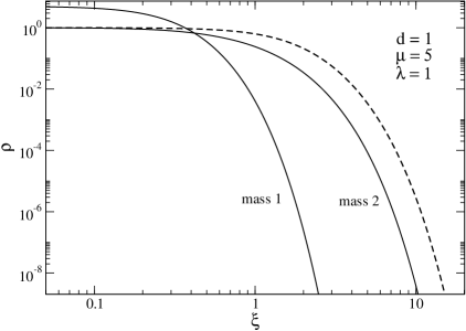
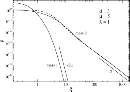
Figure 1: The dimensionless density profiles $\tilde{\rho}_{1}(\xi)=\lambda\mu e^{-\mu\psi}$ and $\tilde{\rho_{2}}(\xi)=e^{-\psi}$ for $\mu=5$ and for $\lambda=1$ in $d=1$ (Fig. 1.a) and $d=3$ (Fig. 1.b). The dashed line represents the density of the one component system.

3.3 The Milne variables

Since the multi-species Emden equation does not satisfy a homology theorem, it cannot be transformed into a first order differential equation as in the one-species case. However, the use of the Milne variables is still useful to analyze the phase portrait of the equation. In the general case, they are defined by

$$u=\frac{d\ln M(r)}{d\ln r}=\xi\frac{\lambda\mu e^{-\mu\psi}+e^{-\psi}}{\psi^{\prime}} v=-\frac{d\ln p(r)}{d\ln r}=\xi\psi^{\prime}\left(\frac{\lambda\mu e^{-\mu\psi}+e^{-\psi}}{\lambda e^{-\mu\psi}+e^{-\psi}}\right),$$ , (42)

where we used the integrated density $M(r)=\int_{0}^{r}\rho S_{d}r^{d-1}\,dr$ and the total pressure $p(r)=(\rho_{1}/m_{1}+\rho_{2}/m_{2})k_{B}T$. Taking the logarithmic derivatives of $u$ and $v$ with respect to $\xi$ and introducing the notation $w=(\lambda e^{-\mu\psi}+e^{-\psi})(\lambda\mu^{2}e^{-\mu\psi}+e^{-\psi})/(\lambda\mu e^{-\mu\psi}+e^{-\psi})^{2}$, we get

$$\frac{1}{u}\frac{du}{d\xi} = \frac{1}{\xi}(d-u-vw),$$ (43)

$$\frac{1}{v}\frac{dv}{d\xi} = \frac{1}{\xi}[u+v(1-w)-(d-2)].$$ (44)

The single species case is recovered for $\lambda=0$ and $w=1$. Taking the ratio of the above equations, we obtain

$$\frac{u}{v}\frac{dv}{du}=\frac{u+v(1-w)-(d-2)}{d-u-vw}.$$ (45)

The solution curve in the $(u,v)$ plane is plotted in Fig. 2. The curve is parameterized by $\xi$. It starts from the point $(u,v)=(d,0)$ with a slope

$$\left(\frac{dv}{du}\right)_{0}=-\frac{d+2}{d}\frac{(1+\lambda\mu)^{3}}{(1+\lambda)[1+\lambda\mu(\mu(1+\lambda\mu)+1)]},$$ (46)

corresponding to $\xi=0$. For $d>2$ and $\xi\rightarrow+\infty$, the curve converges to the limit point $(d-2,2)$ which corresponds to the asymptotic behavior $e^{-\psi}\sim 2(d-2)/\xi^{2}$. Contrary to the single-species case, the ($u,v$) curve can make loops before spiraling around the limit point. These loops are a signature of a multi-components system : using Eq. (45), the points of horizontal and vertical tangent are defined respectively by $u+v(1-w)=d-2$ and $u+vw=d$. Due to the term $w$, new solutions of these equations arise with respect to the single-species case and they create loops. For $d>10$, the $(u,v)$ curve reaches the limit point without spiraling but still makes loops for the reason previously mentioned. For $d<2$, the curve tends monotonically to $(0,+\infty)$ for $\xi\rightarrow+\infty$ as in the single species case. The two-dimensional case is discussed in Sec. 3.5.

  

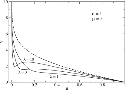
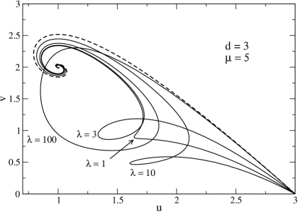
Figure 2: The solution of the two-species Emden equation in the ($u,v$) plane for $d=1$ (left, Fig. 2.a) and in $d=3$ (right, Fig. 2.b). The single-species case is represented by the dashed line.

3.4 The thermodynamical parameters

As indicated previously, isothermal self-gravitating systems have infinite mass. We shall overcome this problem by confining the system within a spherical box of radius $R$ (Antonov model). Physically, the box delimits the region of space where thermodynamical arguments can be applied. In the biological problem (chemotaxis), the box represents the natural boundary of the domain in which the bacteria live. For bounded isothermal systems, the solution of Eq. (33) is terminated by the box at a normalized radius given by $\alpha=(S_{d}Gm_{2}\beta\rho_{2}(0))^{1/2}R$. We shall now determine the temperature and the energy corresponding to the configuration indexed by $\alpha$.

Using the Poisson equation (5), we write the Gauss theorem

$$GM=G\int\rho\,d{\bf r}=S_{d}G\int_{0}^{R}\rho r^{d-1}\,dr=\int_{0}^{R}\frac{d}{dr}\left(r^{d-1}\frac{d\Phi}{dr}\right)\,dr=\left(r^{d-1}\frac{d\Phi}{dr}\right)_{r=R}.$$ (47)

Introducing the dimensionless variables defined previously, we find that the normalized inverse temperature is given by

$$\eta\equiv\frac{\beta GMm_{2}}{R^{d-2}}=\alpha\psi^{\prime}(\alpha).$$ (48)

The calculation of the energy $E=K+W$ is a little more intricate. The kinetic energy is given by

$$K=\frac{d}{2}\left(N_{1}+N_{2}\right)k_{B}T=\frac{d}{2}\left(\frac{M_{1}}{m_{1}}+\frac{M_{2}}{m_{2}}\right)k_{B}T=\frac{d}{2}\frac{M_{2}}{m_{2}}\left(\frac{\chi}{\mu}+1\right)k_{B}T.$$ (49)

Using $M=M_{2}(\chi+1)$ and Eq. (48), the normalized kinetic energy can be written

$$-\frac{KR^{d-2}}{GM^{2}}=-\frac{d}{2\alpha\psi^{\prime}(\alpha)}\frac{\chi+\mu}{\mu(\chi+1)}.$$ (50)

For $d\neq 2$, the expression of the potential energy can be deduced from the Virial theorem

$$2K+(d-2)W=dV_{d}R^{d}p(R),$$ (51)

where $V_{d}=S_{d}/d$ is the volume of a $d$-dimensional sphere with unit radius (and $S_{d}$ is the surface of a $d$-dimensional unit sphere) [3]. Using $p(R)=({\rho_{1}(R)/m_{1}}+{\rho_{2}(R)/m_{2}})k_{B}T$ and the expressions (32) of the density, we directly obtain

$$-\frac{WR^{d-2}}{GM^{2}}=-\frac{1}{(d-2)\psi^{\prime 2}(\alpha)}\left(\lambda e^{-\mu\psi(\alpha)}+e^{-\psi(\alpha)}\right)+\frac{d}{(d-2)\alpha\psi^{\prime}(\alpha)}\frac{{\chi}+{\mu}}{\mu(\chi+1)}.$$ (52)

Adding Eqs. (50) and (52), we find that the total normalized energy is

$$\Lambda\equiv-\frac{ER^{d-2}}{GM^{2}}=\frac{d}{2\alpha\psi^{\prime}(\alpha)}\biggl{(}\frac{4-d}{d-2}\biggr{)}\frac{{\chi}+{\mu}}{\mu(\chi+1)}-\frac{1}{(d-2)\psi^{\prime 2}(\alpha)}\left(\lambda e^{-\mu\psi(\alpha)}+e^{-\psi(\alpha)}\right).$$ (53)

Note that an alternative expression of the potential energy, valid also for $d=2$, can be obtained along the following lines. Starting from the expression

$$W=\frac{1}{2}\int\rho\Phi\,d{\bf r},$$ (54)

and introducing the dimensionless variables defined previously, we get

$$-\frac{WR^{d-2}}{GM^{2}}=-\frac{1}{2\alpha^{d}\psi^{\prime 2}(\alpha)}\int_{0}^{\alpha}\left(\lambda\mu e^{-\mu\psi}+e^{-\psi}\right)(\psi+\psi_{0})\xi^{d-1}\,d\xi,$$ (55)

where $\psi_{0}=m_{2}\beta\Phi(0)$ represents the normalized central gravitational potential. It is determined by the relation $\psi(\alpha)=m_{2}\beta\left(\Phi(R)-\Phi(0)\right)$ with $\Phi(R)=-{GM}/[{(d-2)R^{d-2}}]$ for $d\neq 2$. This yields

$$\psi_{0}=-\biggl{(}\frac{\alpha\psi^{\prime}(\alpha)}{d-2}+\psi(\alpha)\biggr{)}.$$ (56)

Equation (55) remains valid for $d=2$ but in that case, $\Phi(R)=0$ so that $\psi_{0}=-\psi(\alpha)$. The corresponding expression of the total normalized energy is now

$$\Lambda=-\frac{d}{2\alpha\psi^{\prime}(\alpha)}\frac{{\chi}+{\mu}}{\mu(\chi+1)}-\frac{1}{2\alpha^{d}\psi^{\prime 2}(\alpha)}\int_{0}^{\alpha}\left(\lambda\mu e^{-\mu\psi}+e^{-\psi}\right)(\psi+\psi_{0})\xi^{d-1}\,d\xi.$$ (57)

Equations (48) and (53) define a series of equilibria $\beta(E)$ parameterized by the value of the normalized radius $\alpha$, or equivalently by the density contrast ${\cal R}\equiv\rho_{2}(0)/\rho_{2}(R)=e^{\psi(\alpha)}$. Along this series of equilibria, we can either fix the ratio of central densities $\lambda$ or the ratio of total mass $\chi$. These two parameters are related to each other by

$$\chi\equiv\frac{M_{1}}{M_{2}}=\frac{\lambda\mu\int_{0}^{\alpha}\xi^{d-1}e^{-\mu\psi}\,d\xi}{\int_{0}^{\alpha}\xi^{d-1}e^{-\psi}\,d\xi}.$$ (58)

In the framework of statistical mechanics, it is more relevant to fix $\chi$ along the series of equilibria since the total mass of each species is a conserved quantity. Furthermore, it is only under this condition that the turning point argument can be used to settle the stability of the system. Therefore, in the foregoing equations, $\lambda$ must be viewed as an implicit function of $\alpha$ given by

$$\lambda(\alpha)=\frac{\chi}{\mu}\frac{\int_{0}^{\alpha}\xi^{d-1}e^{-\psi}\,d\xi}{\int_{0}^{\alpha}\xi^{d-1}e^{-\mu\psi}\,d\xi}.$$ (59)

Then, for given $\alpha$, the two-species Emden equation (33) must be solved by an iterative procedure in order to satisfy the constraint (59).

  

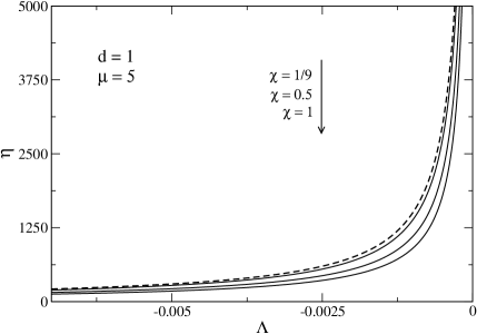
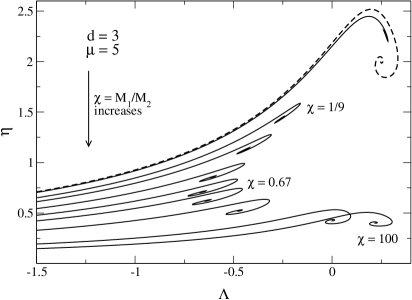
Figure 3: Series of equilibria (caloric curves) for a two-components isothermal gas in $d=1$ (left, Fig. 3.a) and in $d=3$ (right, Fig. 3.b). We plot the inverse normalized temperature $\eta=GMm_{2}\beta/R^{d-2}$ as a function of the normalized energy $\Lambda=-ER^{d-2}/GM^{2}$ for several values of the total mass ratio $\chi=M_{1}/M_{2}$. The dashed curve represents the one component case, i.e. $\chi=0$.

Figure 3 displays an ensemble of caloric curves in $d=1$ and in $d=3$ for different values of $\chi$ (at fixed $\mu$). In $d=1$, the curves are monotonic and the system is always stable. In $d=3$, the curves present turning points at which a mode of stability is lost depending on the ensemble considered (a vertical tangent corresponds to a loss of microcanonical stability and a horizontal tangent to a loss of canonical stability). These results have been discussed in detail for the one-species case, see e.g. [13], and will not be repeated here. We shall just discuss how the critical points (beyond which no equilibrium state exists) depend on the relative mass of the particles. First, consider the canonical ensemble in which the control parameter is the normalized inverse temperature $\eta$. For $\eta>\eta_{c}(\mu,\chi)$, the system undergoes an “isothermal collapse”. For $\chi=0$ we obviously recover the value $\eta_{c}\simeq 2.52$ of the single species case. As the mass ratio $\chi$ increases (at fixed total mass $M$ and $\mu>1$), $\eta_{c}$ decreases ($T_{c}$ increases) up to $\eta_{c}=2.52/\mu$ obtained for $\chi\rightarrow+\infty$. In the microcanonical ensemble, the control parameter is the normalized energy $\Lambda$. For $\Lambda>\Lambda_{c}(\mu,\chi)$, the system undergoes a “gravothermal catastrophe”. For $\chi=0$ and $\chi\rightarrow+\infty$, we recover the single-species value $\Lambda_{c}\approx 0.335$. Between these two extreme values, $\Lambda_{c}$ passes by a minimum $(\Lambda_{c})_{min}(\mu)$. These results are illustrated in Fig. 4 where $\eta_{c}$ and $\Lambda_{c}$ are plotted as a function of $\chi$ for a given value of $\mu$. The value of the minimum of the normalized energy $(\Lambda_{c})_{min}(\mu)$ seems to behave linearly with $\mu$ (except for $\mu\rightarrow 1$) as illustrated in Fig. 5. If we take the particles of mass $m_{2}$ as a reference, we conclude that the onset of isothermal collapse in the canonical ensemble is advanced when heavier particles $m_{1}>m_{2}$ are added to the system (keeping the total mass $M$ fixed). It is delayed if lighter masses ($\mu<1$) are added. On the other hand, the onset of the gravothermal catastrophe in the microcanonical ensemble is always advanced in a multi-species system (with respect to the single species case), whatever the mass of the particles added (keeping the total mass $M$ fixed).

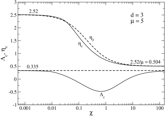
Figure 4: Evolution of the critical normalized inverse temperature $\eta_{c}$ (Jeans temperature) and the critical normalized energy $\Lambda_{c}$ (Antonov energy) as a function of $\chi$ for $d=3$ and $\mu=5$. We plot with a dashed-dotted line the critical temperature $\eta_{J}$ obtained by using the Jeans swindle (see Appendix B for details). Note this “naïve” prediction provides a reasonable fit of the exact critical temperature $\eta_{c}$.

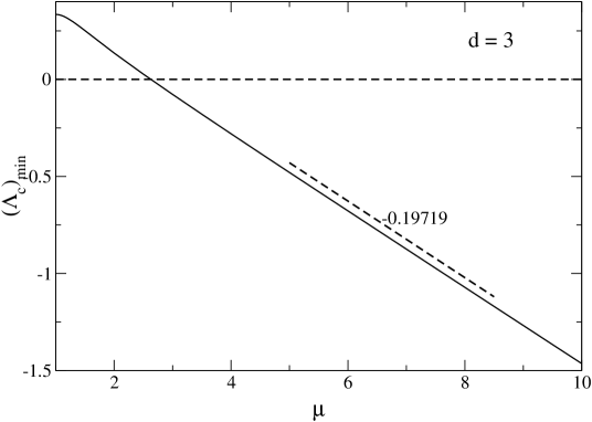
Figure 5: Evolution of the minimum Antonov energy $(\Lambda_{c})_{min}$ as a function of $\mu$ for $d=3$. In the range considered, it decreases approximately linearly as $-0.19719\mu$. Note that the minimum Antonov energy becomes positive for $\mu\simeq 2.627$ and $\chi\simeq 0.68$. Furthermore, the value of $\chi$ for which $\Lambda_{c}$ is minimum is always close to $0.7$ (except for $\mu\rightarrow 1$). This is probably related to the fact that $(\Lambda_{c})_{min}(\mu)$ is almost linear in this range.

Some analytical results can be obtained for $\alpha\rightarrow+\infty$ and $d>2$. This corresponds to the configurations located near the limit point in Fig. 3.b, at the center of the spiral. In that case, it will be shown a posteriori that $\lambda(\alpha)$ diverges for a fixed $\chi$. Accordingly, we can neglect the term $e^{-\psi}$ in the Emden equation (33) which reduces to

$$\frac{1}{\xi^{d-1}}\frac{d}{d\xi}\left(\xi^{d-1}\frac{d\psi}{d\xi}\right)=\lambda\mu e^{-\mu\psi}.$$ (60)

This approximation is valid for $\xi<\xi^{\prime}$, where $\xi^{\prime}$ is such that $\lambda\mu e^{-\mu\psi(\xi^{\prime})}\sim e^{-\psi(\xi^{\prime})}$. If we introduce a new potential $\Theta$ depending on $\zeta\equiv\sqrt{\lambda}\mu\xi$ through the defining relation

$$\psi(\xi)=\frac{1}{\mu}\Theta\left(\zeta\right)=\frac{1}{\mu}\Theta\left(\sqrt{\lambda}\mu\xi\right),$$ (61)

then Eq. (60) takes the form of the ordinary Emden equation

$$\frac{1}{\zeta^{d-1}}\frac{d}{d\zeta}\left(\zeta^{d-1}\frac{d\Theta}{d\zeta}\right)=e^{-\Theta}.$$ (62)

Using the behavior $\Theta\sim 2\ln\zeta-\ln[2(d-2)]$ for large $\zeta$, we obtain the following behavior of $\psi(\xi)$ in the range $1\ll\xi<\xi^{\prime}$:

$$e^{-\psi}\sim\frac{[2(d-2)]^{1/\mu}}{(\sqrt{\lambda}\mu\xi)^{2/\mu}}.$$ (63)

We shall find a posteriori that $\xi^{\prime}\sim\alpha$ so that the range of validity of this behavior is huge in the limit $\alpha\rightarrow+\infty$. This scaling in $\xi^{-2/\mu}$ contrasts from the scaling in $\xi^{-2}$ obtained in the limit $\xi\rightarrow+\infty$ for fixed $\lambda$. The validity of Eq. (63) is confirmed in Fig. 6 where we plot the normalized density profile of a bounded isothermal system for a large value of $\alpha$.

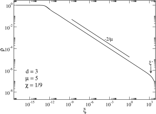
Figure 6: Dimensionless density profile $\tilde{\rho}_{2}(\xi)=e^{-\psi}$ of the lightest particles enclosed within a box for $d=3$, $\mu=5$, $\chi=1/9$ and $\alpha=5000$. In the limit $\alpha\rightarrow+\infty$, the profile decays as $\xi^{-2/\mu}$ for $1\ll\xi<\xi^{\prime}\sim\alpha$. This can be contrasted to the $\xi^{-2}$ decay for $\xi\rightarrow+\infty$ in an open system with fixed $\lambda$ (see Fig. 1).

Using Eqs. (59) and (63), we can investigate the asymptotic behavior of $\lambda(\alpha)$ for $\alpha\rightarrow+\infty$. We have to estimate the two integrals

$$I_{1}(\alpha) = \int_{0}^{\alpha}\xi^{d-1}e^{-\mu\psi}\,d\xi,$$ (64)

$$I_{2}(\alpha) = \int_{0}^{\alpha}\xi^{d-1}e^{-\psi}\,d\xi,$$ (65)

for large values of $\alpha$. We check that for $d>2$ and $\mu>1$, the integrals (extended to $+\infty$) do not converge. Therefore, both terms in the decomposition

$$I_{2}(\alpha)=\int_{0}^{\xi^{\prime}}\xi^{d-1}e^{-\psi}\,d\xi+\int_{\xi^{\prime}}^{\alpha}\xi^{d-1}e^{-\psi}\,d\xi$$ (66)

behave as a power law with the same exponent (the second integral is not negligible with respect to the first). We can obtain the asymptotic behavior of the first integral by using the analytical expression (63) of $\psi$ in the range $1\ll\xi<\xi^{\prime}$. However, since we do not know the expression of $\psi$ for $\xi^{\prime}<\xi<\alpha$, we cannot compute the second integral. Thus we can get the exponent of the power law divergence of $I_{i}(\alpha)$ but not the prefactor.

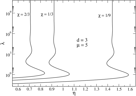
Figure 7: The $\lambda(\eta)$ curves for several values of $\chi=M_{1}/M_{2}$ for $d=3$. These curves are parameterized by $\alpha$.

Evaluating Eqs. (64) and (65) with Eq. (63), we obtain

$$I_{1}(\alpha)\sim K_{1}\frac{\alpha^{d-2}}{\lambda(\alpha)} I_{2}(\alpha)\sim K_{2}\frac{\alpha^{d-{2}/{\mu}}}{\lambda(\alpha)^{{1}/{\mu}}},$$ , (67)

where, for the reasons explained previously, the prefactors are not known. The asymptotic behavior of $\lambda(\alpha)$ is now obtained by substituting Eq. (67) in Eq. (59). This yields

$$\lambda(\alpha)\sim K\alpha^{2(\mu-1)}.$$ (68)

As $\mu>1$, the numerical density ratio $\lambda(\alpha)$ always diverges for $\alpha\rightarrow+\infty$ and $d>2$. This justifies our initial assumptions. If we now insert Eq. (68) in (67), we find that $I_{2}(\alpha)$ diverges as $I_{2}(\alpha)\sim\alpha^{d-2}$. On the other hand, $I_{1}(\alpha)$ behaves as $I_{1}(\alpha)\sim\alpha^{d-2\mu}$ which diverges for $\mu<\mu_{3/2}=d/2$ and tends to zero for $\mu>\mu_{3/2}$. In Fig. 7 we plot the ratio of central numerical densities $\lambda$ as a function of $\eta$ for different values of $\chi$.

3.5 The two-dimensional case

The dimension $d=2$ is a critical dimension for self-gravitating systems [2]. It is also the relevant dimension for the biological problem of chemotaxis, since bacterial colonies usually live on a plate. Therefore, the dimension $d=2$ requires a particular attention. The two-dimensional Emden equation (33) reads

$$\frac{1}{\xi}\frac{d}{d\xi}\left(\xi\frac{d\psi}{d\xi}\right)=\lambda\mu e^{-\mu\psi}+e^{-\psi}.$$ (69)

The density profile behaves asymptotically as $e^{-\psi}\sim A\xi^{-\delta}$ where $A$ and $\delta$ are constants. For $\lambda=0$ (single-species case), Eq. (69) can be solved analytically and we get the exponent $\delta=4$. For other values of $\lambda$, we have $\delta\neq 4$. Some density profiles are plotted in Fig. 8. The phase portrait of the Emden equation (33) in the Milne plane is shown in Fig. 9. On the other hand, the thermodynamical parameters $\eta$ and $\Lambda$ are given by

$$\eta=GMm_{2}\beta=\alpha\psi^{\prime}(\alpha),$$ (70)

$$\Lambda=-\frac{E}{GM^{2}}=-\frac{1}{\alpha\psi^{\prime}(\alpha)}\frac{{\chi}/{\mu}+1}{\chi+1}-\frac{1}{2\alpha^{2}\psi^{\prime 2}(\alpha)}\int_{0}^{\alpha}\left(\lambda\mu e^{-\mu\psi}+e^{-\psi}\right)(\psi-\psi(\alpha))\xi\,d\xi.$$ (71)

Note that the normalized temperature and the normalized energy do not depend on $R$. This is a consequence of the logarithmic form of the gravitational potential in $d=2$. An ensemble of caloric curves are plotted in Fig. 10. As in the previous section, the value of $\chi$ is fixed along a series of equilibria so that $\lambda(\alpha)$ is determined by an iterative procedure. In continuity with the single species case, the caloric curves form a plateau for $\Lambda\rightarrow+\infty$. Thus, there exists a critical inverse temperature $\eta_{c}(\chi,\mu)$ above which no equilibrium state is possible in the canonical ensemble (by contrast, there is no critical energy in $d=2$ in the microcanonical ensemble). The critical temperature $\eta_{c}(\chi,\mu)$ has two expressions depending on whether $\mu>2$ or $\mu<2$ as we now show.

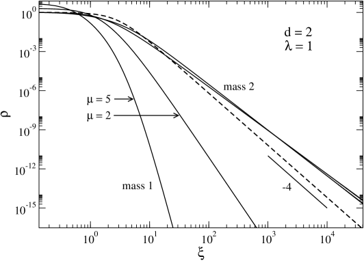
Figure 8: Dimensionless density profiles $\tilde{\rho}_{1}(\xi)=\lambda\mu e^{-\mu\psi}$ and $\tilde{\rho_{2}}(\xi)=e^{-\psi}$ in dimension $d=2$ for $\lambda=1$ and for $\mu=2$ and $\mu=5$. For comparison, the dashed line represents the density of the singe-component system with slope $-4$. The slope of the profile $e^{-\psi}\sim\xi^{-\delta}$ depends on $\lambda$ and $\mu$.

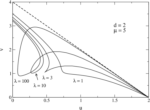
Figure 9: The solution of Eq. (33) in the ($u,v$) plane, where $u$ and $v$ are defined by Eq. (42) for the two-components system at $d=2$. The single-species case is represented by the dashed line. All the curves start at $(u,v)=(d,0)$ with the initial slope given by Eq. (45). For $\xi\rightarrow+\infty$, they tend to the terminal point $(0,\delta)$.

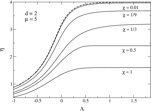
Figure 10: An ensemble of caloric curves for different values of $\chi=M_{1}/M_{2}$ in the two-dimensional case. The dashed curve represents the one-component case.

We first consider the situation in which, at $T=T_{c}$, the two profiles form a Dirac peak at $r=0$. The parameters corresponding to this situation will be found a posteriori. In this case, the critical temperature can be obtained from the Virial theorem as in the single-species problem [3]. We start from the general relation valid in $d=2$ :

$$2K-\frac{GM^{2}}{2}=2p(R)V,$$ (72)

with $V=\pi R^{2}$. If the densities are concentrated in a Dirac peak at $r=0$, the total pressure at the edge of the box vanishes. Equations (49) and (72) directly lead to the result

$$k_{B}T_{c}=\frac{GM^{2}}{4N}.$$ (73)

The critical normalized temperature is

$$\eta_{c}=4\frac{{\chi}+{\mu}}{\mu(\chi+1)}.$$ (74)

For $\chi=0$, we recover the critical inverse temperature $\eta_{c}=4$ obtained for the single-species case [2].

It will be shown that the above regime, called regime (I), corresponds to the case where the function $\lambda(\alpha)$ converges for $\alpha\rightarrow+\infty$. We now consider the regime (II) where $\lambda(\alpha)$ diverges so that Eq. (69) reduces to Eq. (60) with $d=2$. With the change of variables of Eq. (61), we obtain the classical Emden equation (62). In $d=2$, it can be solved analytically and, returning to original variables, we get

$$\psi(\xi)=\frac{2}{\mu}\ln\left(1+\frac{\lambda\mu^{2}}{8}\xi^{2}\right).$$ (75)

This analytical expression provides a good approximation of the solution for all values of $\xi<\xi^{\prime}$ where $\xi^{\prime}$ is such that

$$\int_{0}^{\xi^{\prime}}e^{-\psi(\xi)}\xi\,d\xi\sim\lambda\mu\int_{0}^{\xi^{\prime}}e^{-\mu\psi(\xi)}\xi\,d\xi.$$ (76)

Substituting Eq. (75) into Eq. (76) and using Eq. (78), we find that $\xi^{\prime}\sim\alpha$ so the range of validity of the analytical expression is huge, as checked numerically. The density profile of the lightest particles decreases as $e^{-\psi}\sim\xi^{-4/\mu}$ and the density profile of the heaviest particles decreases as $e^{-\mu\psi}\sim\xi^{-4}$. These heaviest particles form a Dirac peak as $\alpha\rightarrow+\infty$. Furthermore, the density $\lambda\mu e^{-\mu\psi}$ of species $1$ becomes smaller than the density $e^{-\psi}$ of species $2$ for $\xi>\xi^{\prime\prime}\sim\alpha^{-(\mu-2)^{2}/(4(\mu-1))}\rightarrow 0$. In order to determine the asymptotic behavior of $\lambda(\alpha)$ for $\alpha\rightarrow+\infty$, we have to estimate the integrals $I_{1}(\alpha)$ and $I_{2}(\alpha)$ defined by Eqs. (64) and (65). We will consistently show that the assumptions made in regime (II) are only valid for $\mu>2$. Then, it is easy to show that the integral $I_{1}$ extended to $+\infty$ is convergent while the integral $I_{2}$ is divergent. Therefore, by using the profile (75) to evaluate (64) and (65), we obtain the exact asymptotic expression of $I_{1}$ while we only obtain the correct exponent of $\alpha$ in $I_{2}$ but not the prefactor. Indeed, in the calculation of $I_{1}$ the second integral in the decomposition (66) is negligible while in the calculation of $I_{2}$ it is of the same order as the first. Then, we obtain

$$I_{1}(\alpha)\sim\frac{4}{\lambda\mu^{2}} I_{2}(\alpha)\sim K_{2}\lambda^{-2/\mu}\alpha^{{2(\mu-2)}/{\mu}},$$ , (77)

and, using Eq. (59), we get

$$\lambda(\alpha)\sim\left(\frac{\chi K_{2}\mu}{4}\right)^{\frac{\mu}{2}}\alpha^{\mu-2},$$ (78)

for $\alpha\rightarrow+\infty$. The assumption that $\lambda(\alpha)$ diverges is only consistent with $\mu>2$. Note that from Eq. (78) and the value of $I_{1}$, we obtain the exact result $I_{2}\rightarrow 4/\chi\mu$. We also note that $I_{1}\rightarrow 0$ for $\alpha\rightarrow+\infty$.

  

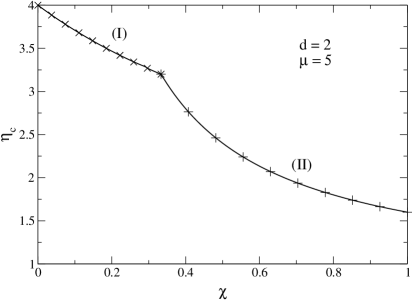
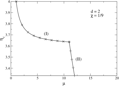
Figure 11: The critical temperature $\eta_{c}$ is plotted versus $\chi$ (Fig. 11.a) and $\mu$ (Fig. 11.b). The solid lines represent the numerical results. They are in excellent agreement with the theoretical results (80) and (74) in the two regimes. The transition between these regimes appears when $\chi=\chi_{*}=1/(\mu-2)$ in Fig. 11.a and when $\mu=\mu_{*}=2+1/\chi$ in Fig. 11.b.

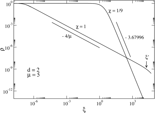
Figure 12: The normalized density profile $\tilde{\rho}_{2}=e^{-\psi}$ is plotted for $\mu=5>2$ and for two different values of $\chi$ situated from both sides of the critical value $\chi_{*}=1/(\mu-2)=1/3$. For $\chi=1/9<\chi_{*}$ (regime I), the asymptotic slope of the profile is $-\eta_{c}=-3.6799$ given by Eq. (74). For $\chi=1>\chi_{*}$ (regime II), the asymptotic slope in the range $1\ll\xi\ll\xi^{\prime}\sim\alpha$ is $-4/\mu=-0.8$, see Eq. (75). The final asymptotic slope in the range $\xi^{\prime}<\xi<\alpha$ is $-\eta_{c}=-8/5$ given by Eq. (80).

We are now able to obtain the critical inverse temperature $\eta_{c}$ in regime (II). In this regime, the heavy particles form a Dirac peak at $r=0$ for $T=T_{c}$ while the light particles extend in the whole box. Since their density is non-zero on the edge of the box, we cannot use the reasoning valid in regime (I). However, the normalized temperature (70) can be written in the form

$$\eta=\beta GMm_{2}=2\pi\beta Gm_{2}\left(1+\frac{1}{\chi}\right)\int_{0}^{R}\rho_{1}(r)\,rd{r}=\lambda\mu\left(1+\frac{1}{\chi}\right)\int_{0}^{\alpha}e^{-\mu\psi}\xi\,d\xi,$$ (79)

where the last integral is precisely $I_{1}(\alpha)$. Using Eq. (77) for $\alpha\rightarrow+\infty$, we get

$$\eta_{c}=\frac{4}{\mu}\left(1+\frac{1}{\chi}\right).$$ (80)

We note the fortunate cancellation of $\lambda$ which allows one to obtain this exact result without detailed knowledge of $K_{2}$. We now have two different expressions of the critical normalized inverse temperature $\eta_{c}$, resp. Eqs. (74) and (80). We find that the crossover between the two regimes is obtained for

$$\chi_{*}=\frac{1}{\mu-2} \mu_{*}=2+\frac{1}{\chi}.$$ , (81)

Applying the Virial theorem in regime (II), we can determine the exact expression of the normalized density of species $2$ on the box. Indeed, using Eqs. (72) and (80), we obtain

$$\alpha^{2}e^{-\psi(\alpha)}\rightarrow\frac{8[\chi(\mu-2)-1]}{\mu^{2}\chi^{2}},$$ (82)

for $\alpha\rightarrow+\infty$. This implies another necessary condition to be satisfied in regime (II), namely $\chi>\chi_{*}$.

In conclusion, regime (I) corresponds to $\mu\leq 2$ and ($\mu>2$ and $\chi<\chi_{*}$) ; in that case, $\lambda(\alpha)$ converges and the critical temperature is given by Eq. (74). Regime (II) corresponds to ($\mu>2$ and $\chi>\chi_{*}$) ; in that case, $\lambda(\alpha)$ diverges and the critical temperature is given by Eq. (80). Equivalently, for a given $\chi$, if $\mu<\mu_{*}$ (regime I) the critical temperature is given by Eq. (74) while if $\mu>\mu_{*}$ (regime II) it is given by Eq. (80). Figure 11 clearly exhibits the cross-over of these two different regimes. The theoretical predictions (74), (80) of the critical temperature are perfectly consistent with the numerical results. We plot the normalized density $\tilde{\rho}_{2}=e^{-\psi}$ in Fig. 12. In the regime (I) where $\lambda(\alpha)$ converges, we have the asymptotic behavior $e^{-\psi}\sim A\xi^{-\delta}$ for $\xi\rightarrow+\infty$. Using the fact that $\xi\psi^{\prime}(\xi)\rightarrow\eta_{c}$ for $\xi\rightarrow+\infty$, we find that $\delta=\eta_{c}$ where $\eta_{c}$ is explicitly given by Eq. (74). In particular, $\delta=\eta_{c}=4$ for the single species case. In the regime (II) where $\lambda(\alpha)$ diverges, we have the asymptotic behavior $e^{-\psi}\sim A\xi^{-4/\mu}$ for $1\ll\xi<\xi^{\prime}$ and $\alpha\rightarrow+\infty$. The final asymptotic slope in the range $\xi^{\prime}<\xi<\alpha$ is $-\eta_{c}$ given by Eq. (80). The numerical results are fully compatible with these predicted values.

We now address the determination of the critical temperature in $d=2$ for a system with more than two types of particles. If all the species collapse on a Dirac peak at $T=T_{c}$ as in regime (I) discussed previously, the critical temperature is again given by Eq. (73) with $N=\sum_{\alpha}N_{\alpha}$ and $M=\sum_{\alpha}N_{\alpha}m_{\alpha}$. The critical normalized inverse temperature $\eta=\beta GMm_{X}$ is

$$\eta_{c}=\frac{4Nm_{X}}{M}.$$ (83)

Alternatively, we can consider the case where $\lambda_{1}(\alpha)$ diverges for $\alpha\rightarrow+\infty$, as in regime (II) discussed previously. To apply the same approximations as before, we need to have $\lambda_{1}\gg\lambda_{i}$ for $i=2,...,X$ where $\lambda_{i}=n_{i}(0)/n_{X}(0)$. Repeating the steps described previously in this more general situation, we find that $\lambda_{1}\rightarrow+\infty$ if $\mu_{1}>2$ and $\lambda_{1}\gg\lambda_{i}$ if $\mu_{1}>2\mu_{i}$. We shall assume that these conditions are fulfilled (i.e. $m_{1}>2m_{2}$). In that case $\lambda_{1}\sim\alpha^{(\mu_{1}-2)}$ and we find by an approach similar to that described previously that

$$\eta_{c}=\frac{4Mm_{X}}{M_{1}m_{1}}.$$ (84)

4 Collapse of a multi-components system

4.1 Self-similar solutions of the two-components Smoluchowski-Poisson system

We now consider the dynamics of a system of self-gravitating Brownian particles. We restrict ourselves to the case of only two types of mass $m_{1}$ and $m_{2}$, as we shall see that the general case of a discrete spectrum of particles is a simple generalization of this problem. We also restrict our analysis to a spatial dimension $d>2$. The dimension $d=2$ is critical and deserves a particular treatment (see [2] for the single species case). As in our previous works, we consider a limit of strong friction $\xi\rightarrow+\infty$ so that the dynamical equations reduce to the two-species Smoluchowski-Poisson system (20). We also restrict ourselves to spherically symmetric solutions. By introducing dimensionless variables, we can set $k_{B}=G=R=M=m_{1}=\xi_{1}=1$ without loss of generality. Then, the problem depends only on the asymmetry parameters $\mu=m_{1}/m_{2}=1/m_{2}$ and $\zeta=\xi_{1}/\xi_{2}=1/\xi_{2}$ and on the temperature $T=1/(\eta\mu)$. With these conventions, the dynamical equations can be written

$$\begin{array}[]{rcl}\displaystyle\frac{\partial\rho_{1}}{\partial t}&=&\displaystyle\nabla\cdot(T\nabla\rho_{1}+\rho_{1}\nabla\Phi),\vspace{6pt}\\ \displaystyle\frac{\partial\rho_{2}}{\partial t}&=&\displaystyle\zeta\nabla\cdot(T\mu\nabla\rho_{2}+\rho_{2}\nabla\Phi),\end{array}$$ (87)

$$\Delta\Phi=S_{d}\rho.$$ (88)

We shall impose a vanishing flux across the surface of the confining sphere. Therefore, the boundary conditions are

$$\begin{array}[]{rcl}\displaystyle\frac{\partial\Phi(0,t)}{\partial r}=0,&&\displaystyle\Phi(1,t)=\frac{1}{2-d},\vspace{6pt}\\ \displaystyle T\frac{\partial\rho_{1}}{\partial r}(1,t)+\rho_{1}(1,t)=0,&&\displaystyle T\mu\frac{\partial\rho_{2}}{\partial r}(1,t)+\rho_{2}(1,t)=0.\end{array}$$ (89)

Using the Gauss theorem, we can rewrite the Smoluchowski-Poisson system (87)-(88) in the form of two integrodifferential equations

$$\begin{array}[]{rcl}\displaystyle\frac{\partial\rho_{1}}{\partial t}&=&\displaystyle\frac{1}{r^{d-1}}\frac{\partial}{\partial r}\left[r^{d-1}\left(T\frac{\partial\rho_{1}}{\partial r}+\frac{\rho_{1}}{r^{d-1}}\int_{0}^{r}S_{d}\rho(r^{\prime})r^{\prime d-1}\,dr^{\prime}\right)\right],\vspace{6pt}\\ \displaystyle\frac{\partial\rho_{2}}{\partial t}&=&\displaystyle\frac{\zeta}{r^{d-1}}\frac{\partial}{\partial r}\left[r^{d-1}\left(T\mu\frac{\partial\rho_{2}}{\partial r}+\frac{\rho_{2}}{r^{d-1}}\int_{0}^{r}S_{d}\rho(r^{\prime})r^{\prime d-1}\,dr^{\prime}\right)\right].\end{array}$$ (92)

The Smoluchowski-Poisson system (92) is also equivalent to a set of two coupled differential equations

$$\begin{array}[]{rcl}\displaystyle\frac{\partial M_{1}}{\partial t}&=&\displaystyle T\left(\frac{\partial^{2}M_{1}}{\partial r^{2}}+\frac{1-d}{r}\frac{\partial M_{1}}{\partial r}\right)+\frac{M_{1}+M_{2}}{r^{d-1}}\frac{\partial M_{1}}{\partial r},\vspace{6pt}\\ \displaystyle\frac{\partial M_{2}}{\partial t}&=&\displaystyle\zeta\left[T\mu\left(\frac{\partial^{2}M_{2}}{\partial r^{2}}+\frac{1-d}{r}\frac{\partial M_{2}}{\partial r}\right)+\frac{M_{1}+M_{2}}{r^{d-1}}\frac{\partial M_{2}}{\partial r}\right],\end{array}$$ (95)

for the quantities

$$M_{\alpha}(r,t)=\int_{0}^{r}\rho_{\alpha}(r^{\prime},t)S_{d}r^{\prime d-1}\,dr^{\prime},$$ (96)

which give the mass of species $\alpha=1,2$ within a sphere of radius $r$. In terms of these variables, the boundary conditions take the form

$$M_{\alpha}(0,t)=0\qquad;\qquad{M_{1}(1,t)}=\frac{\chi}{1+\chi},\qquad M_{2}(1,t)=\frac{1}{1+\chi}.$$ (97)

Note that we shall restrict ourselves to the pre-collapse regime, so that we do not consider the possibility that a Dirac peak forms at $r=0$. A Dirac peak forms in the post-collapse regime for $d>2$ and in $d=2$ (see [4, 2] in the single species case). It will be more convenient to work in terms of the functions $s_{\alpha}(r,t)=M_{\alpha}(r,t)/r^{d}$ which have the dimension of a density. They satisfy

$$\begin{array}[]{rcl}\displaystyle\frac{\partial s_{1}(r,t)}{\partial t}&=&\displaystyle T\left(\frac{\partial^{2}s_{1}}{\partial r^{2}}+\frac{d+1}{r}\frac{\partial s_{1}}{\partial r}\right)+(s_{1}+s_{2})\left(r\frac{\partial s_{1}}{\partial r}+ds_{1}\right),\vspace{6pt}\\ \displaystyle\frac{\partial s_{2}(r,t)}{\partial t}&=&\displaystyle\zeta\left[T\mu\left(\frac{\partial^{2}s_{2}}{\partial r^{2}}+\frac{d+1}{r}\frac{\partial s_{2}}{\partial r}\right)+(s_{1}+s_{2})\left(r\frac{\partial s_{2}}{\partial r}+ds_{2}\right)\right].\end{array}$$ (98)

We look for self-similar solutions of the form

$$s_{1}(r,t)=\rho_{0}(t)S_{1}\left(\frac{r}{r_{0}(t)}\right) s_{2}(r,t)=\rho_{0}^{\alpha/2}(t)S_{2}\left(\frac{r}{r_{0}(t)}\right),$$ , (99)

where $\rho_{0}(t)$ represents the typical central density of species $1$ and $r_{0}(t)$ is the typical core radius (of the two species) defined by

$$\rho_{0}r_{0}^{2}=T.$$ (100)

On physical grounds, we expect that the total density should scale as in the single-species case because, on a coarse-grained scale the fine structure of the mass distribution should not matter (except for a continuous spectrum of mass going from $[0,+\infty[$ with peculiar behavior at the extremes, which is not the case here). Therefore, either the two profiles scale the same manner or one dominates the other. Now, by solving numerically the scaling equation coming from Eqs. (98)-(99), we have found that the problem does not admit any physical solution with $\alpha=2$. Hence one species will dominate the other. We define species $1$ as the one that dominates the dynamics. This choice imposes $\alpha<2$ for the other species. We will give later the conditions on $\mu$ and $\zeta$ for which this requirement is satisfied. Inserting Eq. (99) in Eq. (98) and using the notation $x=r/r_{0}(t)$, the equation for $s_{1}(r,t)$ is transformed into

$$\frac{d\rho_{0}}{dt}S_{1}(x)-x\frac{\rho_{0}}{r_{0}}\frac{dr_{0}}{dt}S^{\prime}_{1}(x) = T\left(\frac{\rho_{0}}{r_{0}^{2}}S^{\prime\prime}_{1}(x)+\frac{d+1}{x}\frac{\rho_{0}}{r_{0}^{2}}S^{\prime}_{1}(x)\right)$$

$$+\left(\rho_{0}S_{1}(x)+\rho_{0}^{\alpha/2}S_{2}(x)\right)\left(x\rho_{0}S^{\prime}_{1}(x)+d\rho_{0}S_{1}(x)\right).$$

For sufficiently high densities, we can neglect the sub-dominant term $\rho_{0}^{\alpha/2}S_{2}(x)$ in the above equation. Then, Eq. (4.1) reduces to

$$\frac{d\rho_{0}}{dt}\biggl{(}S_{1}(x)+\frac{1}{2}xS^{\prime}_{1}(x)\biggr{)} = \rho_{0}^{2}\left(S^{\prime\prime}_{1}(x)+\frac{d+1}{x}S^{\prime}_{1}(x)+xS_{1}(x)S^{\prime}_{1}(x)+dS_{1}^{2}(x)\right),$$

which coincides with the equation obtained in the single-species case [2]. Setting $\rho_{0}^{-2}d\rho_{0}/dt=2$, we find that

$$\rho_{0}(t)=\frac{1}{2}\left(t_{coll}-t\right)^{-1}.$$ (102)

Thus, the central density diverges in a finite time $t_{coll}$. Furthermore, the differential equation for the invariant profile can be solved analytically [2] and we get $S_{1}(x)=S_{0}(x)$ where

$$S_{0}(x)=\frac{4}{d-2+x^{2}}.$$ (103)

Using the preceding results, the differential equation determining the invariant profile of species $2$ is given by the linear second order differential equation

$$\zeta\mu S^{\prime\prime}_{2}(x)+\left[\zeta\left(\frac{\mu(d+1)}{x}+xS_{0}(x)\right)-x\right]S^{\prime}_{2}(x)+\left(d\zeta S_{0}(x)-\alpha\right)S_{2}(x)=0.$$ (104)

For $x\rightarrow+\infty$, we have the asymptotic behavior

$$S_{2}(x)\sim x^{-\alpha}.$$ (105)

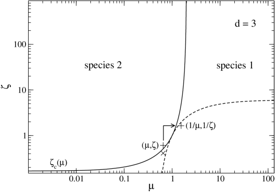
Figure 13: The critical ratio $\zeta_{c}$ as a function of $\mu$ in $d=3$ is plotted in log-log scale. This function starts at $\zeta_{c}(0)=1/6=(d-2)/2d$ and diverges at $\mu=2$. Below the critical line, species $1$ dominates the collapse and above the critical line, species $2$ dominates. In that case, our study can still be used with the transformation $(\zeta,\mu)\rightarrow(1/\zeta,1/\mu)$. This gives a corresponding point located below the dashed curve, corresponding to the function $1/\zeta_{c}(1/\mu)$. We show an example illustrating this transformation when $\zeta>\zeta_{c}$. The (${\times}$) symbol represents the point $(0.65,0.41)$ and the ($+$) symbols represent $(0.65,0.61)$ and $(1/0.65,1/0.61)$ respectively.

Equation (104) can be numerically solved for any couple $(\mu,\zeta)$. As this equation has been obtained under the assumption that the exponent $\alpha<2$, we define a critical ratio of friction coefficients $\zeta_{c}(\mu)$ corresponding to the limit of validity of this hypothesis, i.e. $\alpha(\mu,\zeta_{c})=2$ (similarly, we define $\mu_{c}(\zeta)$ such that $\alpha(\mu_{c},\zeta)=2$).

In the case of a discrete spectrum of particle masses and friction coefficients, the above calculations can be repeated. One obtains an equation identical to Eq. (104) for each type of sub-dominant particles, for which the analysis that we present below has to be applied.

The critical ratio $\zeta_{c}(\mu)$ is plotted in Fig. 13. The value $\zeta_{c}(0)$ can be obtained analytically. Inserting $\mu=0$ and $\alpha=2$ in Eq. (104), we obtain

$$x(\zeta_{c}S_{0}(x)-1)S^{\prime}_{2}(x)+(d\zeta_{c}S_{0}(x)-2)S_{2}(x)=0.$$ (106)

This equation must have a solution for any value of $x$. Taking $x=0$, we find the necessary condition

$$\zeta_{c}(0)=\frac{d-2}{2d}.$$ (107)

Inserting this result in Eq. (106), we find that the scaling profile $S_{2}(x)$ is

$$S_{2}(x)=\frac{A}{(d-2)^{2}/d+x^{2}},$$ (108)

where $A$ is an integration constant. The assumption that species $1$ dominates the collapse is valid for $\zeta<\zeta_{c}(\mu)$. Above this critical line, the role played by the two species is swapped, and species $2$ dominates. We can return to the studied situation by simply changing the index $1\leftrightarrow 2$. Therefore, if $(\mu,\zeta)$ belongs to region $2$ in Fig. 13, this transformation leads to study the case $(1/\mu,1/\zeta)$ which belongs to a sub-part of region $1$, below the dashed line.

We have numerically studied this inversion in Fig. 14. We first start with a value of $(\mu,\zeta)$ below the critical line. Specifically, we take $\mu=0.65$ (leading to $\zeta_{c}\simeq 0.51$) and $\Delta=\zeta-\zeta_{c}=-0.1$ (point $\times$). In that case, species $1$ dominates the collapse : its profile decreases as $\rho_{1}\sim r^{-2}$ while the profile of species $2$ decreases as $\rho_{2}\sim r^{-\alpha}$ with $\alpha=1.85337<2$ determined by solving numerically the scaling equation (104) with $(\mu,\zeta)$. We then increase the value of $\zeta$ above the critical line, at the same distance $\Delta=\zeta-\zeta_{c}=+0.1$ (point $+$). In that case, we have a reversal of population. It is now species $2$ that dominates the collapse : its profile decreases as $\rho_{2}\sim r^{-2}$ while the profile of species $1$ scales as $\rho_{1}\sim r^{-\alpha^{\prime}}$. To get the value of $\alpha^{\prime}$ from our study, we set $2\rightarrow I$ and $1\rightarrow II$. We are now in the situation where species I dominates. Due to this transformation, the new parameters are $\tilde{\mu}\equiv m_{I}/m_{II}=1/\mu$ and $\tilde{\zeta}\equiv\zeta_{I}/\zeta_{II}=1/\zeta$. Then, $S_{I}=S_{2}$ is given by Eq. (103) and $S_{II}=S_{1}$ is solution of Eq. (104) with $\tilde{\mu}$ and $\tilde{\zeta}$. The numerical solution of this scaling equation gives $\alpha^{\prime}=1.74238$. We note that $\alpha^{\prime}\neq\alpha$ so that the slope of the function $\alpha(\Delta)-2$ is discontinuous as $\Delta\rightarrow 0$.

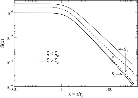
Figure 14: We plot the scaling profiles $S_{1}$ and $S_{2}$ for $\mu=0.65$ and for different values of $\zeta$. We take $\zeta=0.41<\zeta_{c}=0.511070$ (dashed lines) and $\zeta=0.61>\zeta_{c}$ (solid lines). This corresponds to the points marked ${\times}$ and $+$ in Fig. 13. For $\zeta>\zeta_{c}$, the exponent $\alpha^{\prime}$ is obtained from Eq. (104) using the equivalent point $(1/\mu,1/\zeta)$.

For $\mu\rightarrow 2$, the critical ratio $\zeta_{c}(\mu)$ diverges. Therefore, for $\mu>2$, species $1$ always dominates the collapse whatever the value of $\zeta$. It is possible to show the signature of this phenomenon analytically. Assuming $\alpha=2$ and $\zeta_{c}\rightarrow+\infty$, Eq. (104) reduces to

$$S^{\prime\prime}_{2}+\left(\frac{d+1}{x}+\frac{xS_{0}}{\mu}\right)S^{\prime}_{2}+\frac{dS_{0}}{\mu}S_{2}=0.$$ (109)

For large $x$, the profile $S_{2}(x)$ should decay as $x^{-2}$, which immediately implies that $\mu=2$. Equation (109) for $S_{2}(x)$ can then be solved in terms of hypergeometric functions. On the other hand, considering a perturbation expansion $d\rightarrow+\infty$ (see Sec. 4.2), we can obtain the analytical expression

$$\zeta_{c}(\mu)=\frac{1}{2-\mu},\qquad(d\rightarrow+\infty).$$ (110)

We note that, in this limit, $\zeta_{c}(0)=1/2$ in agreement with the exact result (107). We can also obtain an approximate expression of the profile $S_{2}(x)$ for $d\rightarrow+\infty$ (see Sec. 4.2).

4.2 Perturbation expansion for $d\rightarrow+\infty$

We shall first obtain the expression of the scaling exponent $\alpha$ for $d\rightarrow+\infty$. We shall see that the resulting expression applied for $d=3$ already provides a good approximation of the exact solution. We use a method similar to that developed in [2] in a slightly different context. Equation (104) can be formally written as a first order differential equation (writing $S^{\prime\prime}_{2}=(S^{\prime\prime}_{2}/S^{\prime}_{2})S^{\prime}_{2}$) depending on $x$, $S_{0}$ and $S^{\prime\prime}_{2}/S^{\prime}_{2}$,

$$\frac{S^{\prime}_{2}}{S_{2}}=\frac{d\zeta S_{0}(x)-\alpha}{x-\zeta\left[xS_{0}(x)+\mu\left(\frac{d+1}{x}+\frac{S^{\prime\prime}_{2}}{S^{\prime}_{2}}\right)\right]}.$$ (111)

The term $d\zeta S_{0}(x)-\alpha$ vanishes for a particular $x$, noted $x_{0}\neq 0$, whereas the ratio $S^{\prime}_{2}/S_{2}$ cannot vanish. This implies that the denominator in Eq. (111) must be equal to zero for $x=x_{0}$. Using Eq. (103), $x_{0}$ is explicitly given by

$$x_{0}=\sqrt{d\left(\frac{4\zeta}{\alpha}-1\right)+2}.$$ (112)

The condition that the denominator vanishes for this value can be written

$$x_{0}^{2}-\zeta\left[\mu\left(d+1+x_{0}\frac{S^{\prime\prime}_{2}(x_{0})}{S^{\prime}_{2}(x_{0})}\right)+x_{0}^{2}S_{0}(x_{0})\right]=0.$$ (113)

In the sequel, it is more convenient to work with the variable $u=x^{2}$. In terms of this variable, Eqs. (112) and (113) become

$$\displaystyle u_{0}=d\left(\frac{4\zeta}{\alpha}-1\right)+2,$$ (114)

$$\displaystyle u_{0}-\zeta\left[\mu\left(d+2+2u_{0}\frac{S^{\prime\prime}_{2}(u_{0})}{S^{\prime}_{2}(u_{0})}\right)+u_{0}S_{0}(u_{0})\right]=0.$$ (115)

Using Eqs. (103) and (114), Eq. (115) can be rewritten

$$d\left(\frac{4\zeta}{\alpha}-1-\zeta\mu\right)+2\left[1-\zeta\left(1+\mu+\mu d\left(\frac{4\zeta}{\alpha}-1\right)\frac{S^{\prime\prime}_{2}(u_{0})}{S^{\prime}_{2}(u_{0})}+\frac{\alpha}{2}\right)\right]$$

$$-2\left(\zeta\mu\frac{S^{\prime\prime}_{2}(u_{0})}{S^{\prime}_{2}(u_{0})}+\frac{\alpha}{d}\right)=0.$$ (116)

In the limit $d\rightarrow+\infty$, keeping only the dominant terms in the above equation, we obtain $\zeta\mu+1-4\zeta/\alpha=0$ from which we derive the zeroth order expression of $\alpha$

$$\alpha=\frac{4\zeta}{1+\zeta\mu}.$$ (117)

From this last equation, taking $\alpha=2$, we get Eq. (110). Substituting this result in Eq. (111) and keeping only the leading terms for $d\rightarrow+\infty$, we get

$$\frac{S^{\prime}_{2}(u)}{S_{2}(u)}=-\frac{2\zeta}{(d+u)(1+\zeta\mu)}.$$ (118)

This equation is easily integrated and leads to the first approximation of $S_{2}(x)$ in the large $d$ limit

$$S_{2}(x)=\frac{A}{(d+x^{2})^{\frac{2\zeta}{1+\zeta\mu}}}$$ (119)

where $A$ is an integration constant which cannot be determined explicitly at this order. We are now able to obtain the next order correction of $\alpha$. Let us write

$$\alpha=\frac{4\zeta}{1+\zeta\mu}+\frac{\alpha_{1}}{d}.$$ (120)

Inserting this expression in Eq. (4.2), considering the limit $d\rightarrow+\infty$ and using Eqs. (103) and (119), we finally obtain

$$\alpha_{1}=-\frac{8\zeta\left(2\zeta^{2}\mu-\zeta\mu-1\right)}{\left(1+\zeta\mu\right)^{4}}.$$ (121)

This leads to the approximate expression of $\alpha$ to order $1/d$,

$$\alpha=\frac{4\zeta}{1+\zeta\mu}\left[1-\frac{2(2\zeta^{2}\mu-\zeta\mu-1)}{d(1+\zeta\mu)^{3}}+O\left(\frac{1}{d^{2}}\right)\right].$$ (122)

This expression is valid for arbitrary values of $\mu$ and $\zeta$ such that $\alpha<2$.

4.3 Perturbation expansion for $\zeta\sim 1$ and $\mu\sim 1$

We now consider the case of weak asymmetry $\mu\sim 1$ and $\zeta\sim 1$ between the two species for any dimension $d$. In that case, $S_{2}(x)$ will be close to $S_{0}(x)$ and $\alpha$ will be close to $2$. We set

$$\zeta=1-\epsilon\;,\;\mu=1+\eta\;,\;\alpha=2-\epsilon\alpha_{\zeta}-\eta\alpha_{\mu},$$ (123)

$$S_{2}(x)=S_{0}(x)\left[1+\epsilon g_{\zeta}(x)+\eta g_{\mu}(x)\right],$$ (124)

with $\epsilon,\eta\ll 1$. Substituting this expansion in Eq. (104), it is found that the functions $g_{\zeta}(x)$ and $g_{\mu}(x)$ satisfy the first order differential equations (for their derivatives)

$$g^{\prime\prime}_{\zeta}(x)+\left(\frac{d+1}{x}-x\right)g^{\prime}_{\zeta}(x)=\frac{2(d-2)}{d-2+x^{2}}-\alpha_{\zeta},$$ (125)

$$g^{\prime\prime}_{\mu}(x)+\left(\frac{d+1}{x}-x\right)g^{\prime}_{\mu}(x)=\frac{2(d-2)(x^{2}+d+2)}{(d-2+x^{2})^{2}}-\alpha_{\mu}.$$ (126)

We shall discuss these equations separately.

4.3.1 The case $\mu=1$

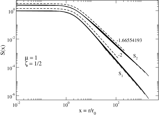
Figure 15: The resolution of the time-dependent equations (95) shows that the evolution is self-similar. We fix for the simulation: $\mu=1$, $d=3$, $T=0.2$, $\zeta=0.5$ and $M_{1}=M_{2}=0.5$. For $t\rightarrow t_{coll}$, the rescaled densities converge to the invariant profiles $S_{1}(x)$ and $S_{2}(x)$ predicted by the theory. The profile of species $1$ is the same as in the one-component problem : $S_{1}(x)=S_{0}(x)\sim x^{-2}$. The profile of species $2$ has been obtained by solving Eq. (104) numerically : $S_{2}(x)\sim x^{-\alpha}$ with $\alpha=1.66554193$.

We first consider the case $\mu=1$. Equations (95) have been solved numerically for $\zeta=1/2$ and the corresponding scaling profiles are plotted in Fig. 15. The numerical results lead to the predicted exponents : at large $x$, $S_{1}(x)\sim x^{-2}$ and $S_{2}(x)\sim x^{-\alpha}$, where $\alpha$ is calculated using Eq. (104). We now consider the weak asymmetry limit $\zeta=1-\epsilon$ with $\epsilon\ll 1$ for $\mu=1$ (the condition $\alpha<2$ imposes $\epsilon>0$). Then, $S_{2}(x)=S_{0}(x)[1+\epsilon g_{\zeta}(x)]$ where $g_{\zeta}(x)$ is the solution of Eq. (125). This equation can be integrated once leading to

$$g^{\prime}_{\zeta}(x)=x^{-(d+1)}e^{x^{2}/2}\int_{0}^{x}y^{d+1}e^{-y^{2}/2}\left(\frac{2(d-2)}{d-2+y^{2}}-\alpha_{\zeta}\right)\,dy.$$ (127)

The integration constant has been determined so as to satisfy the boundary condition $g^{\prime}_{\zeta}(0)=0$. Now, the condition that $g^{\prime}_{\zeta}(x)\rightarrow 0$ as $x\rightarrow+\infty$, leads to an exact expression of $\alpha_{\zeta}$. As $x^{-(d+1)}e^{x^{2}/2}\rightarrow+\infty$ for $x\rightarrow+\infty$, the integral in Eq. (127) has to vanish at large $x$. This yields

$$\alpha_{\zeta}(d)=\frac{\int_{0}^{+\infty}y^{d+1}e^{-y^{2}/2}\frac{2(d-2)}{d-2+y^{2}}\,dy}{\int_{0}^{+\infty}y^{d+1}e^{-y^{2}/2}\,dy}\geq 0.$$ (128)

Note that the integrals can be expressed in terms of $\Gamma$ functions. Rewriting Eq. (127) in the form

$$g^{\prime}_{\zeta}(x)=-x^{-(d+1)}e^{x^{2}/2}\int_{x}^{+\infty}y^{d+1}e^{-y^{2}/2}\left(\frac{2(d-2)}{d-2+y^{2}}-\alpha_{\zeta}\right)\,dy,$$ (129)

we derive the large $x$ behaviors

$$g^{\prime}_{\zeta}(x)\sim\frac{\alpha_{\zeta}}{x} g_{\zeta}(x)\sim\alpha_{\zeta}\ln x.$$ , (130)

We can also carry an expansion of $\alpha_{\zeta}(d)$ in powers of $d^{-1}$ in the limit $d\rightarrow+\infty$. Using the saddle point method in Eq. (128) around the point $y=\sqrt{d+1}$, we obtain

$$\alpha_{\zeta}(d)=1-\frac{3}{2d}-\frac{1}{4d^{2}}-\frac{15197}{25920d^{3}}-\frac{266999}{311040d^{4}}+O\left(\frac{1}{d^{5}}\right).$$ (131)

We can check that the first terms of this expansion reproduce those given by Eq. (122) for $\mu=1$ and $\zeta=1-\epsilon$.

4.3.2 The case $\zeta=1$

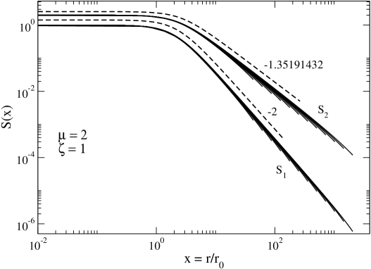
Figure 16: The resolution of the time-dependent equations (95) shows that the evolution is self-similar. We fix for the simulation : $\zeta=1$, $d=3$, $T=0.2$, $\mu=2$ and $M_{1}=M_{2}=0.5$. For $t\rightarrow t_{coll}$, the rescaled densities converge to the invariant profiles $S_{1}(x)$ and $S_{2}(x)$ predicted by the theory. The profile of species $1$ is the same as in the one-component problem : $S_{1}(x)=S_{0}(x)\sim x^{-2}$. The profile of species $2$ has been obtained by solving Eq. (104) numerically : $S_{2}(x)\sim x^{-\alpha}$ with $\alpha=1.35191432$. Note that the large $d$ expansion Eq. (117) leads to $\alpha=4/3$ in fair agreement with the exact numerical result.

We now consider the case $\zeta=1$. Equations (95) have been solved numerically for $\mu=2$ and the corresponding scaling profiles are plotted in Fig. 16. They converge to the invariant profiles predicted by theory. We now consider the weak asymmetry limit $\mu=1+\eta$ with $\eta\ll 1$ for $\zeta=1$ (the condition $\alpha<2$ imposes $\eta>0$). Then, $S_{2}(x)=S_{0}(x)[1+\eta g_{\mu}(x)]$ where $g_{\mu}(x)$ is solution of Eq. (126). Following a procedure similar to that exposed previously, we get the following expression of $\alpha_{\mu}$,

$$\alpha_{\mu}(d)=\frac{\int_{0}^{+\infty}y^{d+1}e^{-y^{2}/2}\frac{2(d-2)(y^{2}+d+2)}{(d-2+y^{2})^{2}}\,dy}{\int_{0}^{+\infty}y^{d+1}e^{-y^{2}/2}\,dy}\geq 0.$$ (132)

and the asymptotic behaviors

$$g^{\prime}_{\mu}(x)\sim\frac{\alpha_{\mu}}{x} g_{\mu}(x)\sim\alpha_{\mu}\ln x.$$ , (133)

The large $d$ expansion of Eq. (132) is

$$\alpha_{\mu}(d)=1+\frac{1}{2d}-\frac{5}{4d^{2}}-\frac{9}{8d^{3}}-\frac{23}{16d^{4}}+O\left(\frac{1}{d^{5}}\right) d\rightarrow+\infty,$$ , (134)

and the first terms of this expansion reproduce those of Eq. (122) for $\zeta=1$ and $\mu=1+\eta$. The exact values of $\alpha_{\zeta}(d)$ and $\alpha_{\mu}(d)$ along with their $O(d^{4})$ expansions are plotted in Fig. 17. For $d=3$, the exact values are $\alpha_{\zeta}(3)=0.437119695$ and $\alpha_{\mu}(3)=0.940162135$.

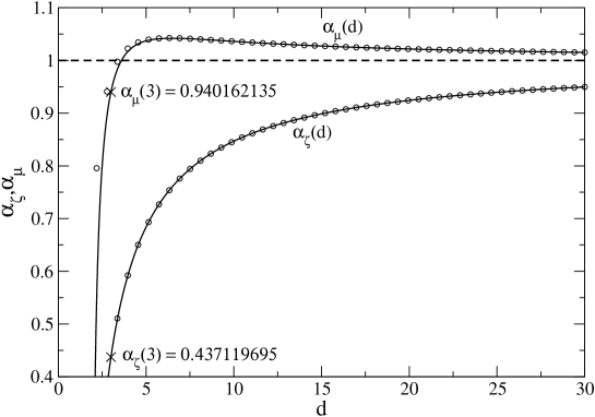
Figure 17: Numerical calculation of $\alpha_{\zeta}$ and $\alpha_{\mu}$ given by Eqs. (128) and (132) as a function of the dimension $d$. The dashed line represents the asymptotic value for $d\rightarrow+\infty$. The $(\circ)$ symbols represent the large $d$ expansion of $\alpha_{\zeta}$ and $\alpha_{\mu}$ to order $d^{-4}$ given in Eqs. (131) and (134).

4.4 Other perturbation expansions

We now consider perturbation expansions of Eq. (104) for small and large values of $\mu$ and $\zeta$. For $\mu\rightarrow 0$ and $\zeta<\zeta_{c}$, Eq. (104) reduces to

$$x(\zeta S_{0}(x)-1)S^{\prime}_{2}(x)+(d\zeta S_{0}(x)-\alpha)S_{2}(x)=0.$$ (135)

Considering the value $x=0$, we get $d\zeta S_{0}(0)-\alpha=0$ leading to

$$\alpha=\frac{4d\zeta}{d-2}.$$ (136)

Then, the scaling profile is given by

$$S_{2}(x)=\frac{A}{(d-2-4\zeta+x^{2})^{2d\zeta/(d-2)}}.$$ (137)

We now wish to examine the limit $\mu\rightarrow+\infty$. We assume that $\alpha\sim 1/\mu$ and check this scaling a posteriori. Using the fact that $S_{2}\sim x^{-\alpha}$ for $x\rightarrow+\infty$ and comparing terms of order $x^{-\alpha-2}$ in Eq. (104), we find that

$$\alpha=\frac{4}{\mu}.$$ (138)

We note that this expression is independent on $\zeta$. The scaling profile obtained from Eq. (104) can be expressed in terms of hypergeometric functions.

In the limit $\zeta\rightarrow 0$, Eq. (104) simplifies into

$$-xS^{\prime}_{2}(x)+(d\zeta S_{0}(x)-\alpha)S_{2}(x)=0.$$ (139)

Considering the value $x=0$, we get

$$\alpha=\frac{4d\zeta}{d-2}.$$ (140)

Then, the scaling profile $S_{2}(x)$ takes the form

$$S_{2}(x)=\frac{A}{(d-2+x^{2})^{2d\zeta/(d-2)}}.$$ (141)

We now wish to examine the limit $\zeta\rightarrow+\infty$ and $\mu>2$. Using the fact that $S_{2}\sim x^{-\alpha}$ for $x\rightarrow+\infty$ and comparing terms of order $x^{-\alpha-2}$, we find that $\mu\alpha^{2}-(4+d\mu)\alpha+4d=0$ leading to $\alpha=d$ or $\alpha=4/\mu$. Since $\alpha<2$, we get

$$\alpha=\frac{4}{\mu}.$$ (142)

Figure 18 shows the functions $\alpha(\zeta=1,\mu)$ and $\alpha(\zeta,\mu=1)$ obtained by solving Eq. (104) in $d=3$ and compares these numerical results with the asymptotic expansions obtained previously. For $\zeta$ and $\mu$ close to 1, the slope of the function $\alpha(\zeta,\mu)$ is given by Eqs. (132) and (128). This figure also confirms the asymptotic expressions (136) and (140) obtained for $\mu\rightarrow+\infty$ and $\zeta\rightarrow 0$.

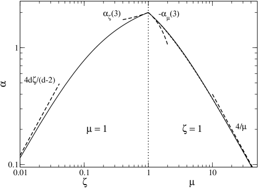
Figure 18: The exponent $\alpha$ is plotted for $\mu=1,\zeta\leq 1$ and for $\mu\geq 1,\zeta=1$ in $d=3$. The dashed lines give the different asymptotic behaviors obtained analytically. Finally, the dotted line for $\zeta=1$ corresponds to the result Eq. (117) of the large $d$ expansion, and is in excellent agreement with the exact value of $\alpha$ (the two curves are almost indistinguishable).

5 Conclusion

In this paper, we have extended previous studies on the thermodynamics of self-gravitating particles in $d$-dimensions to the case of multi-components systems. Our static study applies both to the microcanonical (fixed $E$) and canonical (fixed $T$) ensembles. Thus, it describes ordinary stellar systems (like globular clusters) [32], self-gravitating Brownian particles [1] and bacterial populations [17, 6]. We have investigated how the critical energy (Antonov point) and the critical temperature (Jeans point) depend on the parameters. If we take as a reference a single-species system with particles of mass $m_{2}$ and add particles of mass $m_{1}$ (while removing some particles of mass $m_{2}$ so as to keep the total mass $M$ fixed), we find that the critical temperature is increased if $m_{1}>m_{2}$ and decreased if $m_{1}<m_{2}$ (an analytical estimate of the critical temperature has been obtained in $d>2$ using the Jeans swindle). By contrast, the critical energy is always increased with respect to the single species case in $d>3$. For given ratio $\mu=m_{1}/m_{2}$, it presents a maximum at a certain value of $\chi=M_{1}/M_{2}\simeq 0.7$ (Fig. 3.b). This maximum energy increases roughly linearly with $\mu$ (Fig. 5). As in the one-component case, two-dimensional systems require a specific attention. In $d=2$, there is no collapse in the microcanonical ensemble but there is a collapse in the canonical ensemble below a critical temperature. We have obtained this critical temperature analytically. For $\mu\leq 2$ and for ($\mu>2$ and $\chi<\chi_{*}=1/(\mu-2)$), the two species of particles form a Dirac peak at $T=T_{c}$ and the expression (74) of the critical temperature can be obtained from the Virial theorem. For ($\mu>2$ and $\chi>\chi_{*}=1/(\mu-2)$), only the heaviest particles form a Dirac at $T=T_{c}$ and the expression of the critical temperature (80) is different.

We have also studied the dynamics of self-gravitating Brownian particles (and bacterial populations) in the framework of the two-species Smoluchowski-Poisson system. This corresponds to the canonical ensemble. For $T<T_{c}$, there is no equilibrium state and the system collapses. Looking for self-similar solutions, we have shown that one species dominates the other and collapses as in the single-species problem with a scaling profile $\rho(r)\sim r^{-2}$. The selection of the dominant species is non-trivial. For $\mu>2$, the dominant species is always the one with the heaviest particles. For $\mu<2$, the selection depends on the ratio $\zeta$ of friction parameters as shown in Fig. 13 (for $\zeta=1$, the species with heaviest particles always dominates the collapse). The scaling profile of the “slaved” species decays with an exponent $\alpha<2$ depending on $d$, $\mu$ and $\chi$. This exponent can be calculated numerically by solving Eq. (104). We have also given several asymptotic expansions, see Eqs. (122), (128), (132), (136), (138), (140) and (142).

The generalization of our approach to a continuous spectrum of masses and friction coefficients does not look straightforward. Let us focus on the simpler case of identical friction coefficients. The precise form of the mass spectrum is certainly highly relevant. In particular, we expect that the value of the minimum and maximum masses (possibly 0 and $+\infty$) is crucial. In addition, the behavior of the distribution near the largest mass (for instance $p(m)\sim(m-m_{\rm max})^{-\gamma}$ if $m_{\rm max}$ is finite ($\gamma<1$), $p(m)\sim m^{-\gamma}$ otherwise ($\gamma>1$)) is certainly an important ingredient. However, in the case of a bounded distribution of mass without extravagant singularities, we expect that the results obtained in the present paper will qualitatively hold: the heaviest particles will scale as in the one species case, while lighter particles will scale with a mass dependent exponent less than 2.

Appendix A Derivation of the mean-field equations

In this Appendix, we show that the mean-field approximation used in our study is exact in a proper thermodynamic limit (see [8] in the single species case). We consider the case of self-gravitating Brownian particles described by the stochastic equations (15). The proper statistical ensemble for this system is the canonical ensemble. At equilibrium, the $N$-body distribution function is given by

$$P_{N}(\textbf{r}_{1},\textbf{v}_{1},{...},\textbf{r}_{N},\textbf{v}_{N})=\frac{1}{Z_{T}}e^{-\beta H(\textbf{r}_{1},\textbf{v}_{1},{...},\textbf{r}_{N},\textbf{v}_{N})},$$ (143)

where $Z_{T}$ is the partition function (normalization constant) and $H$ is the Hamiltonian

$$H = \frac{1}{2}\sum_{i=1}^{N}m_{i}v_{i}^{2}+\sum_{i<j}m_{i}m_{j}u(\textbf{r}_{i}-\textbf{r}_{j})=K+U,$$ (144)

where $u(\textbf{r}_{i}-\textbf{r}_{j})=u_{ij}=-{G}/[(d-2)|\textbf{r}_{i}-\textbf{r}_{j}|^{(d-2)}]$ is the gravitational potential. From Eq. (144), it is clear that the velocity distribution is Gaussian. We shall therefore restrict ourselves to the configurational part

$$P_{N}(\textbf{r}_{1},{...},\textbf{r}_{N})=\frac{1}{Z}e^{-\beta U(\textbf{r}_{1},{...},\textbf{r}_{N})}.$$ (145)

We introduce the density probability for particle $i$ of species $\alpha$ to be at $\textbf{r}_{i}$, namely

$$P_{1}^{(\alpha)}(\textbf{r}_{i})=\int P_{N}(\textbf{r}_{1},{...},\textbf{r}_{N})\,\prod_{j\neq i}d{\bf r}_{j}.$$ (146)

Similarly, we define the density probability to find particle $i$ of species $\alpha$ at $\textbf{r}_{i}$ and particle $j$ of species $\alpha^{\prime}$ at $\textbf{r}_{j}$,

$$P_{2}^{(\alpha\alpha^{\prime})}(\textbf{r}_{i},\textbf{r}_{j})=\int P_{N}(\textbf{r}_{1},{...},\textbf{r}_{N})\,\prod_{k\neq i,j}d{\bf r}_{k}.$$ (147)

The total density of particles at r is given by $\rho(\textbf{r})=\sum_{i}m_{i}\delta\left(\textbf{r}-\textbf{r}_{i}\right)$. Its mean value $\left<\rho(\textbf{r})\right>=\sum_{i}\int m_{i}\delta\left(\textbf{r}-\textbf{r}_{i}\right)P_{N}(\textbf{r}_{1},{...},\textbf{r}_{N})\,\prod_{j}d{\bf r}_{j}$ can be written

$$\left<\rho(\textbf{r})\right>=\sum_{\alpha=1}^{X}\sum_{i\in I_{\alpha}}\int m_{\alpha}\delta\left(\textbf{r}-\textbf{r}_{i}\right)P_{1}^{(\alpha)}(\textbf{r}_{i})\,d{\bf r}_{i}=\sum_{\alpha=1}^{X}N_{\alpha}m_{\alpha}P_{1}^{(\alpha)}(\textbf{r})=\sum_{\alpha=1}^{X}{\left<\rho_{\alpha}(\textbf{r})\right>},$$ (148)

where we have defined $I_{\alpha}=\left[g_{\alpha-1}N+1,g_{\alpha}N\right]$ with $g_{0}=0$ and $g_{X}=1$ as the interval of indices labeling particles of species $\alpha$. In the following, we shall work with the mean density. Therefore, we drop the brackets $\left<\cdot\right>$ in order to simplify the notations. Taking the derivative of Eq. (143) with respect to ${\bf r}_{i}$, we get

$$\frac{\partial P_{N}}{\partial\textbf{r}_{i}}=-\beta P_{N}\frac{\partial U}{\partial\textbf{r}_{i}}=-\beta\sum_{j\neq i}P_{N}\ m_{i}m_{j}\frac{\partial u_{ij}}{\partial\textbf{r}_{i}}.$$ (149)

Assuming that $i\in I_{\alpha}$ and integrating over the other variables, we find that

$$\frac{\partial P_{1}^{(\alpha)}}{\partial\textbf{r}_{i}}=-\beta\sum_{j\neq i}\int P_{N}\,m_{i}m_{j}\frac{\partial u_{ij}}{\partial\textbf{r}_{i}}\,\prod_{k\neq i}d{\bf r}_{k} = -\beta\left(N_{\alpha}-1\right)\int P_{2}^{(\alpha\alpha)}(\textbf{r}_{i},\textbf{r}_{2})m_{\alpha}^{2}\frac{\partial u_{i2}}{\partial\textbf{r}_{i}}\,d{\bf r}_{2}$$ (150)

$$-\beta\sum_{\alpha^{\prime}\neq\alpha}N_{\alpha^{\prime}}\int P_{2}^{(\alpha\alpha^{\prime})}(\textbf{r}_{i},\textbf{r}_{2})m_{\alpha}m_{\alpha^{\prime}}\frac{\partial u_{i2}}{\partial\textbf{r}_{i}}\,d{\bf r}_{2}.\qquad\qquad$$

Similarly, we can write an equation for $P_{2}^{(\alpha\alpha^{\prime})}(\textbf{r}_{i},\textbf{r}_{j})$ by integrating Eq. (143) over $N-2$ variables. Then writing

$$P_{2}^{(\alpha\alpha^{\prime})}(\textbf{r}_{i},\textbf{r}_{j})=P_{1}^{(\alpha)}(\textbf{r}_{i})P_{1}^{(\alpha^{\prime})}(\textbf{r}_{j})+P_{2}^{{}^{\prime}(\alpha\alpha^{\prime})}(\textbf{r}_{i},\textbf{r}_{j}),$$ (151)

we can show (see [8] in the single species case) that the cumulating function $P^{\prime}_{2}$ is of order $N_{\alpha}^{-1}$ in the limit

$$N_{\alpha}\rightarrow+\infty\quad{\rm with\ fixed}\quad\eta_{\alpha}=\frac{\beta GM_{\alpha}m_{\alpha}}{R^{d-2}}\quad{\rm and}\quad\mu_{\alpha}=\frac{m_{\alpha}}{m_{X}}.$$ (152)

Thus, in this proper thermodynamic limit, we can make the mean-field approximation

$$P_{2}^{(\alpha\alpha^{\prime})}(\textbf{r}_{i},\textbf{r}_{j})=P_{1}^{(\alpha)}(\textbf{r}_{i})P_{1}^{(\alpha^{\prime})}(\textbf{r}_{j}),$$ (153)

which consists in neglecting the correlations and replacing the two-body distribution function by a product of two one-body distribution functions. Inserting this expression in Eq. (150), we get

$$\frac{\partial P_{1}^{(\alpha)}}{\partial\textbf{r}_{i}}=-\beta m_{\alpha}P_{1}^{(\alpha)}(\textbf{r}_{i})\sum_{\alpha^{\prime}}\int N_{\alpha^{\prime}}P_{1}^{(\alpha^{\prime})}(\textbf{r}_{2})m_{\alpha^{\prime}}\frac{\partial u_{i2}}{\partial\textbf{r}_{i}}\,d{\bf r}_{2}.$$ (154)

Introducing the mean density of each species

$$\rho_{\alpha}({\bf r})=N_{\alpha}m_{\alpha}P_{1}^{(\alpha)}({\bf r}),$$ (155)

and the gravitational potential

$$\Phi({\bf r})=\sum_{\alpha}\int\rho_{\alpha}({\bf r}^{\prime})u({\bf r}-{\bf r}^{\prime})\,d{\bf r}^{\prime},$$ (156)

we can rewrite the above equation in the form

$$\frac{\partial\rho_{\alpha}}{\partial{\bf r}}=-\beta m_{\alpha}\rho_{\alpha}({\bf r})\nabla\Phi({\bf r}).$$ (157)

After integration, we obtain the Boltzmann distribution

$$\rho_{\alpha}({\bf r})=A_{\alpha}e^{-\beta m_{\alpha}\Phi({\bf r})}.$$ (158)

The mean potential energy $W=\left<U\right>$ is given by

$$W=\frac{1}{2}\sum_{i\neq j}\int m_{i}m_{j}\ u_{ij}P_{N}\,\prod_{k=1}^{N}d{\bf r}_{k} = \frac{1}{2}\sum_{\alpha}N_{\alpha}(N_{\alpha}-1)m_{\alpha}^{2}\int P_{2}^{(\alpha\alpha)}(\textbf{r}_{1},\textbf{r}_{2})u_{12}\,d{\bf r}_{1}\,d{\bf r}_{2}$$ (159)

$$+\frac{1}{2}\sum_{\alpha\neq\alpha^{\prime}}N_{\alpha}N_{\alpha^{\prime}}m_{\alpha}m_{\alpha^{\prime}}\int P_{2}^{(\alpha\alpha^{\prime})}(\textbf{r}_{1},\textbf{r}_{2})u_{12}\,d{\bf r}_{1}\,d{\bf r}_{2}.\qquad\qquad$$

Implementing the mean-field approximation (153), valid in the thermodynamic limit, the above expression simplifies into

$$W = \frac{1}{2}\sum_{\alpha,\alpha^{\prime}}N_{\alpha}N_{\alpha^{\prime}}m_{\alpha}m_{\alpha^{\prime}}\int P_{1}^{(\alpha)}({\bf r}_{1})P_{1}^{(\alpha^{\prime})}({\bf r}_{2})u_{12}\,d{\bf r}_{1}\,d{\bf r}_{2},$$ (160)

which can be finally rewritten as

$$W=\frac{1}{2}\int\rho(\textbf{r})\Phi(\textbf{r})\,d{\bf r}.$$ (161)

We now consider the dynamical problem defined by the stochastic equations (15). Using the Kramers-Moyal expansion, the Fokker-Planck equation for the evolution of the $N$-body distribution function $P_{N}({\bf r}_{1},{\bf v}_{1},...,{\bf r}_{N},{\bf v}_{N},t)$ reads

$$\frac{\partial P_{N}}{\partial t}+\sum_{i=1}^{N}\left(\textbf{v}_{i}\cdot\frac{\partial P_{N}}{\partial\textbf{r}_{i}}+{\textbf{F}_{i}}\cdot\frac{\partial P_{N}}{\partial\textbf{v}_{i}}\right)=\sum_{i=1}^{N}\frac{\partial}{\partial\textbf{v}_{i}}\cdot\left(D_{i}\frac{\partial P_{N}}{\partial\textbf{v}_{i}}\ +\xi_{i}P_{N}\textbf{v}_{i}\right),$$ (162)

where $\textbf{F}_{i}=-(1/m_{i})\nabla_{i}U$ is the force by unit of mass (acceleration) acting on particle $i$. We note that the stationary solution of Eq. (162) is the canonical distribution (143) provided that the coefficients of friction and diffusion are related to each other according to the Einstein formula

$$D_{i}=\frac{\xi_{i}}{\beta m_{i}}.$$ (163)

Taking $i\in I_{\alpha}$ and integrating over the other variables, we get

$$\frac{\partial P_{1}^{(\alpha)}}{\partial t}+\textbf{v}_{i}\cdot\frac{\partial P_{1}^{(\alpha)}}{\partial\textbf{r}_{i}}+\int{\textbf{F}_{i}}\cdot\frac{\partial P_{N}}{\partial\textbf{v}_{i}}\,\prod_{k\neq i}d{\bf r}_{k}d{\bf v}_{k}=\frac{\partial}{\partial\textbf{v}_{i}}\cdot\left(D_{\alpha}\frac{\partial P_{1}^{(\alpha)}}{\partial\textbf{v}_{i}}+\xi_{\alpha}P_{1}^{(\alpha)}\textbf{v}_{i}\right).$$ (164)

Now

$$I\equiv\int{\bf F}_{i}P_{N}\prod_{k\neq i}d{\bf r}_{k}\,d{\bf v}_{k} = -\int(N_{\alpha}-1)m_{\alpha}\frac{\partial u_{i2}}{\partial{\bf r}_{i}}P_{2}^{(\alpha\alpha)}({\bf r}_{i},{\bf v}_{i},{\bf r}_{2},{\bf v}_{2},t)\,d{\bf r}_{2}\,d{\bf v}_{2}$$ (165)

$$-\sum_{\alpha^{\prime}\neq\alpha}\int N_{\alpha^{\prime}}m_{\alpha^{\prime}}\frac{\partial u_{i2}}{\partial{\bf r}_{i}}P_{2}^{(\alpha\alpha^{\prime})}({\bf r}_{i},{\bf v}_{i},{\bf r}_{2},{\bf v}_{2},t)\,d{\bf r}_{2}\,d{\bf v}_{2}.$$

From the $N$-body Fokker-Planck equation (162), we can obtain an equation for the time evolution of the two-body distribution function $P_{2}^{(\alpha\alpha^{\prime})}({\bf r}_{i},{\bf v}_{j},{\bf r}_{j},{\bf v}_{j},t)$ and again show that, in the proper thermodynamic limit, the mean-field approximation (153) becomes exact. In that case, the expression of $I$ simplifies into

$$I=-P_{1}^{(\alpha)}({\bf r}_{i},{\bf v}_{i},t)\int\sum_{\alpha^{\prime}}N_{\alpha^{\prime}}m_{\alpha^{\prime}}P_{1}^{(\alpha^{\prime})}({\bf r}_{2},{\bf v}_{2},t)\frac{\partial u_{i2}}{\partial{\bf r}_{i}}\,d{\bf r}_{2}\,d{\bf v}_{2}=P_{1}^{(\alpha)}({\bf r}_{i},{\bf v}_{i},t)\langle{\bf F}\rangle_{i},$$ (166)

where $\left<\textbf{F}\right>_{i}=-\nabla_{i}\Phi$ is the mean force (by unit of mass) acting on particle $i$. Introducing the distribution function

$$f_{\alpha}({\bf r},{\bf v},t)=N_{\alpha}m_{\alpha}P_{1}^{(\alpha)}({\bf r},{\bf v},t),$$ (167)

the mean-field Fokker-Planck equation takes the form

$$\frac{\partial f_{\alpha}}{\partial t}+\textbf{v}\cdot\frac{\partial f_{\alpha}}{\partial\textbf{r}}+\left<\textbf{F}\right>\cdot\frac{\partial f_{\alpha}}{\partial\textbf{v}}=\frac{\partial}{\partial\textbf{v}}\cdot\left(D_{\alpha}\frac{\partial f_{\alpha}}{\partial\textbf{v}}+\xi_{\alpha}f_{\alpha}\textbf{v}\right).$$ (168)

In the strong friction limit, the stochastic equations of motion are given by Eq. (19). In that case, the $N$-body Fokker-Planck equation reads

$$\frac{\partial P_{N}}{\partial t}=\sum_{i=1}^{N}\frac{\partial}{\partial\textbf{r}_{i}}\cdot\left(D^{\prime}_{i}\frac{\partial P_{N}}{\partial\textbf{r}_{i}}+\mu_{i}{P_{N}}\nabla_{i}U\right).$$ (169)

We note that the stationary solution of this equation is given by the configurational part of the canonical distribution (143) provided that the diffusion coefficient and the mobility are related to each other by the Einstein relation

$$D^{\prime}_{i}=\frac{\mu_{i}}{\beta}.$$ (170)

Assuming that $i\in I_{\alpha}$ and integrating over the other variables, we get

$$\frac{\partial P_{1}^{(\alpha)}}{\partial t}=\frac{\partial}{\partial\textbf{r}_{i}}\cdot\left(D^{\prime}_{\alpha}\frac{\partial P_{1}^{(\alpha)}}{\partial\textbf{r}_{i}}+\mu_{\alpha}\int P_{N}\nabla_{i}U\prod_{j\neq i}d{\bf r}_{k}\right).$$ (171)

Evaluating the last term in the mean-field approximation as done previously, we find that

$$\frac{\partial P_{1}^{(\alpha)}}{\partial t}=\frac{\partial}{\partial\textbf{r}_{i}}\cdot\left(D^{\prime}_{\alpha}\frac{\partial P_{1}^{(\alpha)}}{\partial\textbf{r}_{i}}+\mu_{\alpha}m_{\alpha}P_{1}^{(\alpha)}\nabla_{i}\Phi\right),$$ (172)

which is clearly the same as

$$\frac{\partial\rho_{\alpha}}{\partial t}=\frac{1}{\xi_{\alpha}}\nabla\cdot\left(\frac{k_{B}T}{m_{\alpha}}\nabla\rho_{\alpha}+\rho_{\alpha}\nabla\Phi\right).$$ (173)

Appendix B Estimate of the critical temperature using the Jeans swindle

In this Appendix, we extend the original Jeans instability criterion to the case of a multi-components system. We make the Jeans swindle, assuming that the unperturbed state is infinite and homogeneous. Then, we use this criterion to obtain an estimate of the critical temperature $T_{c}$ of an inhomogeneous isothermal multi-components self-gravitating system confined within a box.

Let us consider a small perturbation around an equilibrium state of the two-components Smoluchowski-Poisson system. The linearized equations for the perturbation can be written

$$\begin{array}[]{rcl}\displaystyle\frac{\partial\delta\rho_{1}}{\partial t}&=&\displaystyle\frac{1}{\xi_{1}}\nabla\cdot\left(\frac{k_{B}T}{m_{1}}\nabla\delta\rho_{1}+\rho_{1}\nabla\delta\Phi+\delta\rho_{1}\nabla\Phi\right),\vspace{6pt}\\ \displaystyle\frac{\partial\delta\rho_{2}}{\partial t}&=&\displaystyle\frac{1}{\xi_{2}}\nabla\cdot\left(\frac{k_{B}T}{m_{2}}\nabla\delta\rho_{2}+\rho_{2}\nabla\delta\Phi+\delta\rho_{2}\nabla\Phi\right),\end{array}$$ (174)

where $\rho$ and $\Phi$ refer to the equilibrium state. They have to be completed with the linearized Poisson equation

$$\Delta\delta\Phi=S_{d}G\delta\rho.$$ (175)

These equations are exact but they remain complicated if the static solution is inhomogeneous. They can be solved (semi-analytically) for a one-component system [13] but the generalization to a multi-components system is not straightforward. We shall invoke here the Jeans swindle and consider that the equilibrium state is infinite and homogeneous although this does not rigorously satisfy the equations at zeroth order. With this simplifying assumption, using Eq. (175), the linearized equations (174) take the form

$$\begin{array}[]{rcl}\displaystyle\frac{\partial\delta\rho_{1}}{\partial t}&=&\displaystyle\frac{1}{\xi_{1}}\left(\frac{k_{B}T}{m_{1}}\Delta\delta\rho_{1}+\rho_{1}S_{d}G\delta\rho\right),\vspace{6pt}\\ \displaystyle\frac{\partial\delta\rho_{2}}{\partial t}&=&\displaystyle\frac{1}{\xi_{2}}\left(\frac{k_{B}T}{m_{2}}\Delta\delta\rho_{2}+\rho_{2}S_{d}G\delta\rho\right).\end{array}$$ (176)

Writing the perturbation as $\delta\rho_{\alpha}\sim e^{i(\textbf{k}\cdot\textbf{r}-\omega t)}$, we get

$$\begin{array}[]{rcccccc}\displaystyle\left(-i\omega\xi_{1}+\frac{k_{B}T}{m_{1}}k^{2}-S_{d}G\rho_{1}\right)\delta\rho_{1}-{S_{d}G}\rho_{1}\delta\rho_{2}=0,\vspace{6pt}\\ \displaystyle-{S_{d}G}\rho_{2}\delta\rho_{1}+\left(-i\omega\xi_{2}+\frac{k_{B}T}{m_{2}}k^{2}-S_{d}G\rho_{2}\right)\delta\rho_{2}=0.\end{array}$$ (177)

The cancellation of the determinant of the above system determines the dispersion relation. One can show that $\gamma=-i\omega$ is real so it represents either the growth rate of the perturbation ($\gamma>0$) or its exponential damping ($\gamma<0$) . The point of marginal stability $\omega=0$ is obtained for the Jeans wavevector

$$k^{2}_{J}=\frac{S_{d}G\left(m_{1}\rho_{1}+m_{2}\rho_{2}\right)}{k_{B}T}.$$ (178)

More generally, for a multicomponent system, we have found that

$$k^{2}_{J}=\frac{S_{d}G}{k_{B}T}\sum_{\alpha=1}^{X}m_{\alpha}\rho_{\alpha}.$$ (179)

The criterion of instability $-i\omega\geq 0$ is equivalent to $k\leq k_{J}$. In terms of the wavelength $\lambda=2\pi/k$, it can be written

$$\lambda^{2}\geq\lambda^{2}_{J}=\frac{4\pi^{2}k_{B}T}{S_{d}G\left(m_{1}\rho_{1}+m_{2}\rho_{2}\right)}$$ (180)

This criterion means that if the size of the perturbation $\lambda$ is larger than the critical value $\lambda_{J}$, the gravitational attraction will prevail over diffusion and the system will collapse. If we now return to our original problem, namely an isothermal system enclosed within a box of radius $R$, a naïve application of the above criterion indicates that the system is unstable if $R>\lambda_{J}$. Introducing the total mass of each species through the relation $\rho_{\alpha}\sim M_{\alpha}/R^{d}$, this criterion can be rewritten in terms of the temperature as

$$T\leq T_{c}\equiv K_{d}\frac{G(m_{1}M_{1}+m_{2}M_{2})R^{2-d}}{k_{B}}.$$ (181)

As noticed in [13], the critical temperature $T_{c}$ marking the gravitational instability of box-confined isothermal systems can be related to the Jeans instability criterion by the above argument. Of course, this naïve approach cannot catch the numerical constant $K_{d}$ which appears in the expression of the critical temperature. However, this constant can be obtained from the numerical study of the single species case in $d=3$ where we have $T_{c}=GMm/2.52k_{B}R$ [13]. Thus, we take $K_{3}=1/2.52$. Now, the interest of our treatment for a multi-components system is that we can obtain the dependence of the critical temperature with $\mu$ and $\chi$. Returning to dimensionless variables, we get the instability criterion

$$\eta\geq\eta_{J}=2.52\frac{1+\chi}{1+\chi\mu},$$ (182)

where $\eta_{J}$ is the critical inverse temperature obtained by using the Jeans swindle. This expression returns the single-species result for $\chi=0$ and for $\mu=1$. It is also consistent with the single-species result for $\chi\rightarrow+\infty$ if we redefine $\eta$ with $m_{1}$ instead of $m_{2}$. If we consider the limit $\mu\rightarrow 0$ or $+\infty$ with fixed $N_{1}/N_{2}$, then $\chi=(N_{1}/N_{2})\mu\rightarrow 0$ or $+\infty$, and we again recover the single species case. More generally, we see in Fig. 4 that this approximate expression gives a fair agreement with the exact solution. This is quite satisfying in view of the approximations made to arrive at Eq. (182) (we have assumed that the system is homogeneous). The relative success of this naïve approach is explained by the fact that in $d=3$ the system is weakly inhomogeneous at $T_{c}$. By contrast, the expression (182) does not work at all in $d=2$ (compare with the exact values (74) and (80)) because the system tends to a Dirac peak at $T=T_{c}$.

References

- [1] P.-H. Chavanis, C. Rosier, C. Sire, Phys. Rev. E 66, 036105 (2002).
- [2] C. Sire, P.-H. Chavanis, Phys. Rev. E 66, 046133 (2002).
- [3] P.-H. Chavanis, C. Sire, Phys. Rev. E 69, 016116 (2004).
- [4] C. Sire, P.-H. Chavanis, Phys. Rev. E 69, 066109 (2004).
- [5] P.-H. Chavanis, C. Sire, Phys. Rev. E 70, 026115 (2004).
- [6] P.-H. Chavanis, M. Ribot, C. Rosier, C. Sire, Banach Center Publ. 66, 103 (2004).
- [7] C. Sire, P.-H. Chavanis, Banach Center Publ. 66, 287 (2004).
- [8] P.-H. Chavanis, (2004) [condmat/0409641].
- [9] P.-H. Chavanis, A&A 356, 1089 (2000).
- [10] P.-H. Chavanis, J. Sommeria, R. Robert, Astrophys. J. 471, 385 (1996).
- [11] G. Kurizki, S. Giovanazzi, D. O’Dell, A.I. Artemiev, New regimes in cold gases via laser-induced long-range interactions, in Dynamics and Thermodynamics of Systems with Long Range Interactions, edited by T. Dauxois, S. Ruffo, E. Arimondo, M. Wilkens, Lecture Notes in Physics Vol. 602, Springer (2002).
- [12] G. Kurizki, Int. J. Mod. Phys. B 18, 2027 (2004)
- [13] P.-H. Chavanis, A & A 381, 340 (2002).
- [14] P.-H. Chavanis, Phys. Rev. E 65, 056123 (2002).
- [15] E. Keller, L.A. Segel, J. theor. Biol. 26, 399 (1970).
- [16] W. Jäger, S. Luckhaus, Trans. Am. Math. Soc. 329, 819 (1992).
- [17] J.D. Murray, Mathematical Biology (Springer, 1991).
- [18] J. Katz, Found. Phys. 33, 223 (2003).
- [19] V.A. Antonov, Vest. Leningr. Gos. Univ. 7, 135 (1962).
- [20] D. Lynden-Bell and R. Wood, Mon. Not. R. astr. Soc. 138, 495 (1968).
- [21] L. G. Taff, H. M. Van Horn, C. J. Hansen, R. R. Ross, Astrophys. J. 197, 651 (1975).
- [22] H. J. De Vega, J. A. Siebert, Phys. Rev E 66, 016112 (2002).
- [23] K. R. Yawn, B. N. Miller, Phys. Rev. E 68, 056120 (2003).
- [24] H. Kandrup, Astrophys. J. 244, 316 (1981).
- [25] P.-H. Chavanis, Physica A 332, 89 (2004).
- [26] P.-H. Chavanis, P. Laurençot, M. Lemou, Physica A 341, 145 (2004).
- [27] P.-H. Chavanis, Phys. Rev. E 68, 036108 (2003).
- [28] G. Wolansky, European J. Appl. Math. 13, 641 (2002).
- [29] P.-H. Chavanis, A&A, 432, 117 (2005).
- [30] T. Padmanabhan, Phys. Rep. 188, 285 (1990).
- [31] P.-H. Chavanis, A & A 401, 15 (2003).
- [32] J. Binney and S. Tremaine, Galactic Dynamics (Princeton Series in Astrophysics, 1987).