Finite-size scaling exponents in the interacting boson model

Abstract

We investigate the finite-size scaling exponents for the critical point at the shape phase transition from U(5) (spherical) to O(6) (deformed $\gamma$-unstable) dynamical symmetries of the Interacting Boson Model, making use of the Holstein-Primakoff boson expansion and the continuous unitary transformation technique. We compute exactly the leading order correction to the ground state energy, the gap, the expectation value of the $d$-boson number in the ground state and the $E2$ transition probability from the ground state to the first excited state, and determine the corresponding finite-size scaling exponents.

The interest in the study of quantum phase transitions (QPT) has kept growing in the last years in different branches of quantum many-body physics, ranging from macroscopic systems like quantum magnets, high-$T_{\mathrm{c}}$ superconductors Vojta (2003) or dilute Bose and Fermi gases Romans et al. (2004) to mesoscopic systems such as atomic nuclei or molecules Iachello and Zamfir (2004). Although, strictly speaking QPT only occur in macroscopic systems, there is a renewed interest in studying structural changes in finite-size systems where precursors of the transition are already observed Casten and Zamfir (2000). The understanding of the modifications on the characteristics of the QPT induced by finite-size effects is of crucial importance to extend the concept of phase transitions to finite systems.

In the present study, we analyze these finite-size corrections in the Interacting Boson Model (IBM) of nuclei Iachello and Arima (1987), but the same technique can be applied to other boson systems, for instance to the molecular vibron model Iachello and Levine (1995), or to a multilevel boson model of Bose-Einstein condensates where similar QPT take place Dukelsky and Schuck (2001).

The IBM is a two-level boson model that includes an angular momentum $L=0$ boson (scalar $s$-boson) and five angular momentum $L=2$ bosons (quadrupole $d$-bosons) separated by an energy gap. The $s$ and $d$-bosons represent $s$ and $d$ wave idealized Cooper nucleon pairs. The algebraic structure of this model is governed by the U(6) group and the model has three dynamical symmetries in which the Hamiltonian, written in terms of the invariant (Casimir) operators of a nested chain of subgroups of U(6), is analytically solvable. The dynamical symmetries are named by the first subgroup in the chain: U(5), SU(3) and O(6). The classical or thermodynamic limit of the model was investigated by using an intrinsic state formalism that introduces the shape variables $\beta$ and $\gamma$ Ginocchio and Kirson (1980); Dieperink et al. (1980); Bohr and Mottelson (1980). Within this geometric picture the U(5), SU(3) and O(6) dynamical symmetries correspond to spherical, axially deformed and deformed $\gamma$-unstable shapes, respectively. Transition between two of these dynamical symmetry limits are described in terms of a Hamiltonian with a control parameter that mixes the Casimir operators of the two dynamical symmetries. As a function of the control parameter, the system crosses smoothly a region of structural changes in the ground state wave function for finite number $N$ of bosons. In the large $N$ limit, the smooth crossover turns into a sharp QPT between two well defined shape phases Dieperink et al. (1980); Feng et al. (1981); Frank (1989); López-Moreno and Castaños (1996); Jolie et al. (2002). In particular, the transition from U(5) to O(6) has been intensively studied in recent years because it has a unique second order QPT López-Moreno and Castaños (1996); Jolie et al. (2002); Arias et al. (2003a) associated with a triple point in the IBM parameter space Jolie et al. (2002). Furthermore, it was early recognized that the IBM Hamiltonian along this transition was fully integrable Alhasid and Whelan (1991), and exactly solvable Pan and Draayer (1997); Dukelsky and Pittel (2001).

Unfortunately, it is difficult to use the exact solution to compute finite-size corrections analytically. Thus, we follow a different route which is based on the Continuous Unitary Transformations (CUTs) Wegner (1994); Głazek and Wilson (1993, 1994). Within this framework, we compute the first correction beyond the standard Random Phase Approximation (RPA) Dukelsky et al. (1984) which already contains the key ingredients to analyze the critical point. As already observed in a similar context, Dusuel and Vidal (2004, 2005a, 2005b), this $1/N$ expansion becomes, at this order, singular when approaching the critical region so that one gets nontrivial scaling exponents for the physical observables (ground state energy, gap, occupation number, transition rates). In a second step, we take advantage of the exact solvability of the model to obtain numerical results for large number of bosons which allows us to check our analytical predictions.

Let us consider the U(5)-O(6) transitional Hamiltonian

$$H=x\,n_{d}+\frac{1-x}{4(N-1)}\left(P^{\dagger}_{d}-P^{\dagger}_{s}\right)\left(P^{\phantom{\dagger}}_{d}-P^{\phantom{\dagger}}_{s}\right),$$ (1)

where $n_{d}$ $\sum_{\mu}d^{\dagger}_{\mu}d^{\phantom{\dagger}}_{\mu}$ (with $\mu=-2,-1,0,1,2$) is the $d$-boson number operator, $P^{\dagger}_{s}={s^{\dagger}}^{2}$ and $P^{\dagger}_{d}=\sum_{\mu}(-1)^{\mu}d^{\dagger}_{\mu}d^{\dagger}_{-\mu}$ ; $x$ is the control parameter that mixes the U(5) linear Casimir operator ($x=1$) with the O(6) quadratic Casimir operator ($x=0$). The system undergoes a QPT at $x_{\mathrm{c}}=1/2$, between a U(5) (spherical) phase for $1/2\leq x\leq 1$ and a O(6) (deformed $\gamma$-unstable) phase for $0\leq x\leq 1/2$, when $N\to\infty$ López-Moreno and Castaños (1996); Jolie et al. (2002); Arias et al. (2003a).

In the following, we shall restrict our analysis to the spherical (symmetric) phase which allows to investigate the critical point more simply than from the deformed phase. The Holstein-Primakoff boson expansion of one-body boson operators is especially well-suited to perform a $1/N$ expansion of the boson Hamiltonian (1). In the present case, it reads Holstein and Primakoff (1940); Klein and Marshalek (1991)

$$d^{\dagger}_{\mu}d^{\phantom{\dagger}}_{\nu} = b^{\dagger}_{\mu}b^{\phantom{\dagger}}_{\nu},$$ (2a)

$$s^{\dagger}s = N-\sum_{\mu}d^{\dagger}_{\mu}d^{\phantom{\dagger}}_{\mu}=N-\sum_{\mu}b^{\dagger}_{\mu}b^{\phantom{\dagger}}_{\mu}=N-n_{b},\quad\quad$$ (2b)

$$d^{\dagger}_{\mu}s = N^{1/2}b^{\dagger}_{\mu}(1-n_{b}/N)^{1/2}=(s^{\dagger}d^{\phantom{\dagger}}_{\mu})^{\dagger}.$$ (2c)

Keeping terms of order $(1/N)^{0}$ in the Hamiltonian expressed in terms of the new $b$’s yields a quadratic Hamiltonian which can be diagonalized via a Bogoliubov transformation. One then recovers RPA results Dukelsky et al. (1984); Rowe (2004). At the next order $(1/N)^{1}$, the Hamiltonian is quartic and diagonalizing it clearly requires a more sophisticated method. To achieve this goal, we used the CUTs technique Wegner (1994); Głazek and Wilson (1993, 1994). For an introduction to this method, we refer the reader to Refs. Dusuel and Vidal (2004, 2005a, 2005b) where CUTs were applied in a similar context. One introduces a running Hamiltonian

$$H(l) = E_{0}(l)+\Delta(l)n_{b}+V(l):n_{b}^{2}:+W(l)P^{\dagger}_{b}P^{\phantom{\dagger}}_{b}$$

$$+\Gamma(l)\left(P^{\dagger}_{b}+P^{\phantom{\dagger}}_{b}\right)+\Lambda(l)\left(P^{\dagger}_{b}n_{b}+n_{b}P^{\phantom{\dagger}}_{b}\right),\quad$$

which is related to the initial Hamiltonian $H(0)$ through a unitary transformation, namely $H(l)=U^{\dagger}(l)H(0)U(l)$. This transformation $U$ is chosen such that $H(\infty)$ commutes with $n_{b}$. In Eq. (Finite-size scaling exponents in the interacting boson model), $:\mathcal{O}:$ denotes the normal ordered form of the operator $\mathcal{O}$, and the notations for the $b$’s are the same as for the $d$’s. The evolution of the running Hamiltonian is obtained from the flow equation $\partial_{l}H(l)=[\eta(l),H(l)]$, where $\eta(l)=\partial_{l}U^{\dagger}(l)U(l)$ is the anti-hermitian generator of the unitary transformation. For the problem at hand, we consider the so-called quasi-particle conserving generator Knetter and Uhrig (2000),

$$\eta(l)=\Gamma(l)\left(P^{\dagger}_{b}-P^{\phantom{\dagger}}_{b}\right)+\Lambda(l)\left(P^{\dagger}_{b}n_{b}-n_{b}P^{\phantom{\dagger}}_{b}\right),$$ (4)

designed to ensure $H(\infty)$ commutes with $n_{b}$, i.e. $\Gamma(\infty)=\Lambda(\infty)=0$.

The flow equations can be solved exactly, order by order in $1/N$, and the coefficients of the final Hamiltonian are found to be

$$E_{0}(\infty) = \frac{N(1-x)}{4}+\frac{5}{2}\left[\frac{1}{2}(1-3x)+\Xi(x)^{1/2}\right]$$

$$+ \frac{5x(1-x)}{N}\left[\frac{25x-9}{16\Xi(x)}-\frac{1}{\Xi(x)^{1/2}}\right],$$

$$\Delta(\infty) = \Xi(x)^{1/2}+\frac{x(1-x)}{N}\left[\frac{9x-1}{4\Xi(x)}-\frac{2}{\Xi(x)^{1/2}}\right],\quad$$ (6)

$$V(\infty) = \frac{x^{2}(1-x)}{4N\Xi(x)},$$ (7)

$$W(\infty) = \frac{x(1-x)(3x-1)}{8N\Xi(x)},$$ (8)

where $\Xi(x)=x(2x-1)$. One can then straightforwardly analyze the low-energy spectrum.

The ground state of $H(\infty)$ is the state $|0\rangle$ with zero $b$-bosons, whose energy is $E_{0}(\infty)$. The first excited state is five-fold degenerate and corresponds to one quadrupole boson $b^{\dagger}_{\mu}|0\rangle$, whose excitation energy is $\Delta(\infty)$. These are the five components of the first $2^{+}$ excited state. For the two-boson states, things are a bit more complicated because of the $W$ term which is not diagonal in the basis of states $\{b^{\dagger}_{\mu}b^{\dagger}_{\nu}|0\rangle\}$ with $\mu,\nu=-2,-1,0,1,2$. It is however easy to see that $P^{\dagger}_{b}P^{\phantom{\dagger}}_{b}$has a nontrivial action only in the subspace $\Big{\{}b^{\dagger}_{2}b^{\dagger}_{-2}|0\rangle,b^{\dagger}_{1}b^{\dagger}_{-1}|0\rangle,\frac{1}{\sqrt{2}}{b^{\dagger}_{0}}^{2}|0\rangle\Big{\}}$. The corresponding $3\times 3$ matrix has eigenvalues $0$ (twice) and $10$. One thus finds that there are 14 degenerate states with excitation energy $2[\Delta(\infty)+V(\infty)]$, and one $0^{+}$ state which is given by $\frac{1}{\sqrt{10}}P^{\dagger}_{b}|0\rangle$ with energy $2[\Delta(\infty)+V(\infty)+5W(\infty)]$. Let us emphasize that the degeneracy is lifted at order $(1/N)^{1}$, an effect missed at the RPA order. The 14 degenerate states are the 9 components of the first excited $4^{+}$ state and the 5 components of the second excited $2^{+}$ state. These $4_{1}^{+}$ and $2_{2}^{+}$ states are degenerate along the whole transition line because of the common O(5) structure. Note also that, at fixed $N$, the $0^{+}_{2}$ state degenerates with the $4_{1}^{+}$ and $2_{2}^{+}$ in the U(5) limit. This low-energy spectrum is depicted in Fig. 1 for $N=40$. The agreement between numerics and analytical results is pretty good and has been checked to improve when $N$ gets bigger, as long as one is sufficiently far away from the critical point. Indeed, as can be seen in (Finite-size scaling exponents in the interacting boson model-8), the $1/N$ order corrections diverge at $x=1/2$. This singular behavior already found in other models Dusuel and Vidal (2004, 2005a, 2005b) is a signature of the noninteger scaling exponents Rowe et al. (2004) that we discuss below.

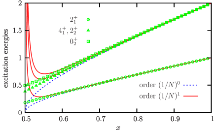
Figure 1: Comparison between analytical results (solid and dotted lines) and the numerical results (circle, triangle and square symbols) for the first excitation energies, with $N=40$.

The main strength of the CUTs is to allow the computation of expectation values of observables as well as transition amplitudes. Thus, one has to perform the unitary transformation of the observables in which one is interested. In the present case, all observables can be deduced from the knowledge of the flow of the operator $b^{\dagger}_{\mu}(l)=U^{\dagger}(l)b^{\dagger}_{\mu}U(l)$. For example, the average number of $d$-bosons in the ground-state of the Hamiltonian $H$ is found as $\langle n_{d}\rangle=\langle 0|\sum_{\mu}b^{\dagger}_{\mu}(\infty)b^{\phantom{\dagger}}_{\mu}(\infty)|0\rangle$. This quantity can also be computed using the Hellmann-Feynman theorem which yields $\langle n_{d}\rangle=\frac{\partial}{\partial y}{[(1+y)E_{0}]}$ with $y=x/(1-x)$. One then gets

$$\langle n_{d}\rangle = \frac{5}{2}\left[\frac{3x-1}{2\Xi(x)^{1/2}}-1\right]$$

$$+\frac{5x(1-x)^{2}}{16N}\left[-\frac{7x}{\Xi(x)^{2}}+\frac{8}{\Xi(x)^{3/2}}\right].$$

However, this theorem cannot be applied to compute nondiagonal matrix elements such as transition amplitudes. To illustrate the power of the CUTs for such a task, we focus on the $B(E2)$ transition probability between the ground state and the first excited state which is defined as $B(E2)=5\big{|}\langle 2,0|Q_{0}^{(2)}|0,0\rangle\big{|}^{2}$ in the standard $|J,M\rangle$ basis, with $Q_{0}^{(2)}=s^{\dagger}d^{\phantom{\dagger}}_{0}+d^{\dagger}_{0}s$. The flow equations for $b^{\dagger}_{\mu}(l)$ can still be exactly integrated out order by order in $1/N$ and leads to:

$$B(E2) = N\frac{5x}{\Xi(x)^{1/2}}$$

$$+5x^{2}\left[-\frac{27x^{2}-20x+5}{4\Xi(x)^{2}}+\frac{4x-1}{\Xi(x)^{3/2}}\right].$$

The comparison between analytical and the numerical $B(E2)$ transition probabilities for a system of $N=40$ bosons, is shown in Fig. 2.

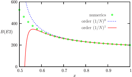
Figure 2: Comparison between analytical results (solid dotted lines) and the numerical results (circles) for the $B(E2)$ transition probability, with $N=40$.

As for the excitation energies, there are divergences in the $B(E2)$ values at the critical point, although they now appear even at the RPA order Rowe (2004). However, at finite $N$ values no divergence should appear in the physical magnitudes or their derivatives with respect to the control parameter $x$, even at the critical point. This obvious remark allows us to determine the nontrivial scaling exponents. Such an analysis was proposed in Refs. Dusuel and Vidal (2004, 2005a, 2005b), and we shall now briefly recall how it works. The $1/N$ expansion of any physical quantity $\Phi$ has two contributions, the regular (reg) and singular (sing) respectively, when $x$ approaches the critical value $x_{\mathrm{c}}=1/2$:

$$\Phi_{N}(x)=\Phi_{N}^{\mathrm{reg}}(x)+\Phi_{N}^{\mathrm{sing}}(x).$$ (11)

A close analysis of the singular part in the vicinity of the critical point $x_{\mathrm{c}}$ shows that the singular part scales as

$$\Phi_{N}^{\mathrm{sing}}(x)\simeq\frac{\Xi(x)^{\xi_{\Phi}}}{N^{n_{\Phi}}}\mathcal{F}_{\Phi}\left[N\Xi(x)^{3/2}\right],$$ (12)

where $\mathcal{F}_{\Phi}$ is a function depending on the scaling variable $N\Xi(x)^{3/2}$ only. To compensate the singularity coming from $\Xi(x)^{\xi_{\Phi}}$ (or its derivative), one thus must have $\mathcal{F}_{\Phi}(x)\sim x^{-2\xi_{\Phi}/3}$ so that $\Phi_{N}^{\mathrm{sing}}(x_{\mathrm{c}})\sim N^{-(n_{\Phi}+2\xi_{\Phi}/3)}$. In Table 1 the computed scaling exponents for the low energy physical quantities studied are summarized.

$\Phi$	$\xi_{\Phi}$	$n_{\Phi}$	$-(n_{\Phi}+2\xi_{\Phi}/3)$
$E_{0}$	1/2	0	-1/3
$\Delta$	1/2	0	-1/3
$\langle n_{d}\rangle$	-1/2	0	1/3
$B(E2)$	-1/2	-1	4/3

Table 1: Scaling exponents for the ground state energy $E_{0}$, the gap $\Delta$, the number of $d$-bosons in the ground- state $\langle n_{d}\rangle_{GS}$ and the $B(E2)$ transition probability.

In order to check these results, it is important to analyze the large $N$ behavior of $\Phi_{N}$. Therefore, we have numerically solved the problem by diagonalizing the boson Hamiltonian (1) up to $N=1000$. Details of this calculation will be given in a forthcoming publication Dusuel et al. . As can be seen in Fig. 3, an excellent agreement is found between the exponents predicted analytically and the numerical results.

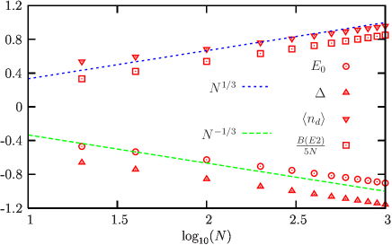
Figure 3: Plot of the singular parts of $E_{0}$, $\Delta$, $\langle n_{d}\rangle$ and $B(E2)/(5N)$ at the critical point $x_{c}=1/2$, in a $\log_{10}-\log_{10}$ scale.

Let us underline that the scaling exponent for the ground state energy has been recently obtained by Rowe et al. Rowe et al. (2004) by using the collective model associated to the IBM Hamiltonian Arias et al. (2003b). This mapping onto a quartic potential also explains why we found the same finite-size scaling exponent for the ground state energy and the gap ($1/3$) in other similar models Dusuel and Vidal (2004, 2005a, 2005b). However, such an approach does not allow to simply compute the finite $N$ corrections and may not be suitable to obtain the behavior for observables such as $B(E2)$. The CUTs method is thus, in this context, a very useful tool.

In the present work, we have exactly computed finite-size corrections beyond the RPA in the symmetric phase of the IBM model. We have shown that the spectral properties at the critical point in the U(5)-O(6) transition have well-defined asymptotic limits and we have calculated the $N$-dependent scale factors. A natural extension of this work would be to investigate the broken phase ($x<1/2$) but the presence of Goldstone modes in the low-energy spectrum (at the RPA level) makes it more involved Dusuel et al. .

The study of the scaling properties at the critical point of a QPT of a finite-$N$ particle model is of primer interest in several mesoscopic systems like nuclei, molecules, and other physical systems. The present results provide a tool to tackle such a study and to characterize the approach of the system to the critical regions as the number of particles goes to infinity.