Does the potential energy landscape of a supercooled liquid resemble a collection of traps?

Abstract

It is analyzed whether the potential energy landscape of a glass-forming system can be effectively mapped on a random model which is described in statistical terms. For this purpose we generalize the simple trap model of Bouchaud and coworkers by dividing the total system into M weakly interacting identical subsystems, each being described in terms of a trap model. The distribution of traps in this extended trap model (ETM) is fully determined by the thermodynamics of the glass-former. The dynamics is described by two adjustable parameters, one characterizing the common energy level of the barriers, the other the strength of the interaction. The comparison is performed for the standard binary mixture Lennard-Jones system with 65 particles. The metabasins, identified in our previous work, are chosen as traps. Comparing molecular dynamics simulations of the Lennard-Jones system with Monte Carlo calculations of the ETM allows one to determine the adjustable parameters. Analysis of the first moment of the waiting distribution yields an optimum agreement when choosing $M\approx 3$ subsystems. Comparison with the second moment of the waiting time distribution, reflecting dynamic heterogeneities, indicates that the sizes of the subsystems may fluctuate.

I Introduction

Understanding the properties of supercooled liquids and in particular the nature of the glass transition is still a major scientific challenge. An important concept to grasp the important physics is related to the potential energy landscape (PEL) Goldstein (1969); Debenedetti and Stillinger (2001); Wales (2003). In this view the system is regarded as a point in the high-dimensional configuration space. At sufficiently low temperatures the system is mainly characterized by the different minima (inherent structures) of the PEL and their respective harmonic attraction basins Stillinger and Weber (1982); Sciortino et al. (1999); Büchner and Heuer (1999); Mossa et al. (2002). With the advent of faster computers in recent years it became possible to elucidate the properties of the minima and the saddles and thus to relate the thermodynamic Sciortino et al. (1999); Büchner and Heuer (1999); La Nave et al. (2002a); Starr et al. (2001) as well as the dynamic behavior of supercooled liquids Scala et al. (2000); Keyes (1994); Heuer (1997); Broderix et al. (2000); Schrøder et al. (2000); La Nave et al. (2001); Angelani et al. (2002); Wales and Doye (2001); Denny et al. (2003); Doliwa and Heuer (2003a, b, c); Nave and Sciortino (2004) to the properties of the PEL. Most of the work has been devoted to the study of the thermodynamics. From analyzing the PEL for different densities it was possible, e.g., to extract the equation of state over a very broad range of temperatures and pressures Starr et al. (2001); La Nave et al. (2002b).

The Adam-Gibbs relation constitutes a relation between the dynamics and the thermodynamics Adam and Gibbs (1965). It expresses the relaxation time in terms of the configurational entropy. This relation seems to hold rather well for different systems Sastry (2001); Scala et al. (2000); Giovambattista et al. (2003). The theoretical relevance, however, is not clear so far. Therefore it is still an open question which properties of the PEL beyond the distribution of inherent structures determine the dynamic behavior Stillinger and Debenedetti (2002).

It has been attempted to fill this gap between thermodynamics and dynamics by phenomenological models for which the system is hopping between discrete states like for the random-energy model or the trap model Dyre (1995); Monthus and Bouchaud (1996); Odagaki (1995). Here we are in particular interested in the trap model as discussed by Monthus and Bouchaud Monthus and Bouchaud (1996). This model starts from a distribution $G(e)$ of traps with depth $e$. The average waiting time in a trap of depth $e$ is given by $\tau(e,T)=\tau_{0}\exp(\beta V(e))$ where $V(e)=b-e$ and $b$ is the common barrier level. After thermal excitation the system randomly chooses a neighbor trap; see Fig.1 for a one-dimensional sketch. The trap energies are randomly distributed. Of course, for a real system one has to consider a distribution of traps in high-dimensional space. At low temperatures the slow dynamics is related to very long residence times in deep traps. Most work has been devoted to exponentially distributed traps but different distributions $G(e)$ can be chosen as well. In any event, $G(e)$ fully determines the thermodynamic properties and should reflect the energy-distribution of inherent structures. A priori, it is not clear whether the trap model is of major relevance for describing the PEL of real glass-forming liquids. From a conceptual point of view an important property of the trap model is its non-topographic nature. The arrangement of traps is purely statistical and the dynamics is exclusively related to the properties of the individual traps and not to possibly subtle correlations among adjacent traps. We mention in passing, that in alternative approaches the dynamics is rationalized without any reference to thermodynamic properties Garrahan and Chandler (2002).

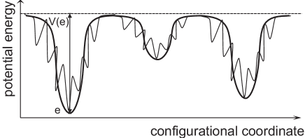
Figure 1: Thick line: Sketch of the standard trap model. Thin line: The traps are identified as the metabasins and typically contain several inherent structures.

A very detailed analysis of the dynamics naturally involves the properties of the barriers between the inherent structures as well as the topology of the PEL. For a binary-mixture Lennard Jones system (BMLJ) trajectories, generated via molecular dynamics simulations, have been analyzed in detail. It is immediately visible that during very long times the system resides in some fixed region of the configurational space. Thus the dynamics is restricted to simple back and forth jumps between a finite number of inherent structures Büchner and Heuer (2000); Denny et al. (2003); Doliwa and Heuer (2003b). It is useful to regard such a set of inherent structures as an elementary state, denoted metabasin (MB) Stillinger (1995); Middleton and Wales (2001); Doliwa and Heuer (2003a); Saksaengwijit et al. (2003). The energy and configuration of a MB is taken from the inherent structure of this MB with the lowest energy. Finally, the total trajectory of the system in configuration space can be regarded as a sequence of different MB, each characterized by an energy and a waiting time. Actually, some work has been recently performed to relate this configurational space picture to real space dynamics Middleton and Wales (2001); Reinisch and Heuer (2004a, b); Vogel et al. (2004); Trygubenko and Wales (2004) and to explain the response to applied strain in glasses with the help of the concept of MB Osborne and Lacks (2004).

Here we would like to remind the reader of a remarkable result, presented in previous work Doliwa and Heuer (2003b). It turns out that for all relevant temperatures analyzed so far,

$$\sum_{i=1}^{N}\langle(r_{i}(n)-r_{i}(0))^{2}\rangle\approx a^{2}n.$$ (1)

The left term denotes the mean square displacement after n MB-transitions and $a^{2}$ is the temperature-independent average distance between two adjacent MB in configuration space. Two important consequences follow from Eq. 1: (i) On the level of MB the dynamics of the BMLJ system can be described as a random walk in configuration space; (ii) The diffusion constant can be expressed as Doliwa and Heuer (2003b)

$$D(T)=a^{2}/6\langle\tau(T)\rangle.$$ (2)

Thus knowledge of the average waiting time is sufficient to predict the macroscopic dynamics. Actually, the simplicity of these results can serve as the a posteriori justification for the introduction of the MB approach because on the level of inherent structures no simple physical picture can be formulated for the dynamics of the BMLJ system Doliwa and Heuer (2003b). Recent work for a pure Lennard-Jones system of significantly smaller size seems to indicate that there the random-walk like dynamics already holds on the level of inherent structures Keyes and Chowdhary (2001).

Another remarkable result is the fact that a BMLJ system with $N=65$ particles has no relevant finite size effects for the dynamics in the accessible temperature range for computer simulationsDoliwa and Heuer (2003d). In particular, a system with $N=130$ particles behaves like an independent superposition of two systems with $N=65$ particles. Therefore it is sufficient to study the PEL of the BMLJ system with $N=65$ particles. Actually, when choosing even smaller systems (e.g. $N=40$) significant finite-size effects occur Büchner and Heuer (1999).

Maybe the simplest disordered model, reproducing the observed features, is the trap model as introduced above. Since the distribution of traps is fully determined by the thermodynamics of the system, the dynamics is basically governed by a single parameter, namely the barrier height $b$. In any event, if the PEL can be mapped on a trap model, the MB have to be identified as traps; see Fig.1. Recent simulation work for the BMLJ system directly shows in different ways that on a quantitative level the predictions of the trap model are neither compatible with the distribution of waiting times Denny et al. (2003) nor with the activation energy $V(e)=b-e$ Doliwa and Heuer (2003a).

The scope of this work is twofold. First, we will use general arguments to define an extended version of the trap model. It fulfills some basic requirements which any model for glass-forming systems should fulfill. Second, by detailed comparison with the properties of the BMLJ system we elucidate to which level this extended trap model will be able to explain the BMLJ dynamics. From the remaining differences important information about the nature of the PEL can be derived. Among other things the concept of dynamic heterogeneities is related to properties of the PEL in a detailed way. Finally, some possible applications of the present results will be indicated.

II The BMLJ system

II.1 Definition

The BMLJ system is one of the standard glass-forming systems used in computer simulations. It contains 80% large and 20% small particles. We use the potential parameters as outlined in Ref.Kob and Andersen (1995); Doliwa and Heuer (2003a). We have performed molecular dynamic simulations for temperatures between $T=0.4$ and $T=1$ with system size $N=65$ and using periodic boundary conditions. Here we present data for $T\geq 0.45$. All units are given in LJ units. The mode-coupling temperature for this model is $T_{c}\approx 0.45$ Götze and Sjogren (1992); Doliwa and Heuer (2003b). As shown in previous work this system size is large enough to reproduce the macroscopic behavior of the BMLJ at least for $T\geq T_{c}$.

II.2 Some previous results

The most important quantity for the thermodynamics is the effective density of MB, i.e. $G(e)$. In previous work it turned out that to a very good approximation

$$G(e)\propto\exp(-(e-e_{0})^{2}/2\sigma_{0}^{2})$$ (3)

with $e_{0}=-279.2$ and $\sigma_{0}^{2}=9.05$ in Lennard-Jones units Sciortino et al. (1999); Büchner and Heuer (1999); Doliwa and Heuer (2003a). From entropy arguments one can estimate that $G(e)$ has a low-energy cutoff around $e=-306$. From $G(e)$ one can calculate the Boltzmann probability $p(e,T)$ that at some randomly chosen time the system visits a MB of energy $e$ at temperature $T$ via

$$p(e,T)\propto G(e)\exp(-e/T).$$ (4)

Note that $G(e)$ is slightly different from the real density of MB due a small dependence of the local curvature of the different MB on their energy $e$ Sciortino et al. (1999); Büchner and Heuer (1999). We just mention in passing that basically the same results for the thermodynamics are obtained if inherent structures rather than MB are analyzed.

In previous simulations we have analyzed in detail the waiting time of the system in MB of energy $e$. Averaging over different MB with energy $e$ we have found the relation

$$\langle\tau(e,T)\rangle=\tau_{0}(e)\exp(\beta V_{eff}(e)),$$ (5)

i.e. the average waiting time in a MB of energy $e$ shows simple Arrhenius behavior. The function $V_{eff}(e)$ can be interpreted as the average saddle height when leaving a MB of energy $e$. This function is reproduced in Fig.2. Note that it was possible to identify the saddles in the PEL which give rise to the specific values of $V_{eff}(e)$. For $e<-295$ the function $V_{eff}(e)$ is linear in $e$ with slope -0.55. In the high-energy limit $V_{eff}(e)$ approaches a constant close to 1. This reflects the fact that the dynamics in high-energy states resembles a non-activated fluid-like dynamics. Using this choice of $V_{eff}(e)$ it is possible to formally describe this fluid-like dynamics as transitions between MB Doliwa and Heuer (2003a). A similar limiting value is reported in Chowdhary and Keyes (2004). In the same energy range the effective prefactor $\tau_{0}(e)$ increases by one order of magnitude Doliwa and Heuer (2003a).

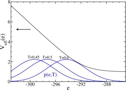
Figure 2: The function $V_{eff}(e)$ as obtained for the BMLJ system together with the distribution $p(e,T)$ for three different temperatures.

As shown in Doliwa and Heuer (2003c) the dynamics is governed by activated processes for $T\leq 0.6$. Correspondingly, the average waiting time is dominated by the escape from low-energy MB ($e\leq-295$). For temperatures below $T_{c}$ it becomes difficult to obtain equilibrium data. Therefore we restrict our detailed analysis to temperatures between 0.45 and 0.6 to compare the dynamics of the BMLJ system with the predictions of the modelling. In Fig.2 we have also included the distributions $p(e,T)$ in this temperature range, obtained from Eq.4. On the low-energy side the contribution stems from few events with relatively large waiting times. Thus energy-dependent observables for, say, $e<-300$ possess rather large statistical errors. In the detailed analysis of the subsequent sections we consider MB with $e\in[-300,-295]$.

III Extended Trap Model: Definition and interpretation

III.1 General aspects of statistical models

How do properties of the PEL translate into dynamics? According to the landscape paradigm the properties of glass-forming systems are reflected by the properties of the minima. As discussed above, we would use the MB rather than the minima as the basic objects. In any event, one has an exponentially large but finite number of states. In the most detailed description the dynamics out of some state $i$ is governed by two temperature dependent functions. First, the probability function $r(...,i\rightarrow j)$ describes the probability that the next state visited is state $j$. The dots indicate that in principle this probability may also depend on the history before entering state $i$. Second, the waiting time in state $i$ is characterized by the distribution function of the waiting times $f(\tau|...,i\rightarrow j)$ when going from state $i$ to state $j$.

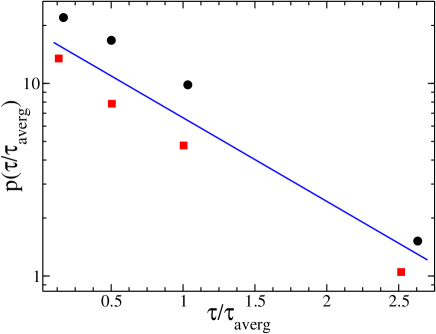
Figure 3: The probability distribution of waiting times for two randomly chosen MB. The time-axis has been normalized by the respective average value $\tau_{averg}$. A perfect exponential waiting time distribution with slope -1 has been included. For better visibility the curves are shifted against each other. 60 escape events have been analyzed for each MB.

Of particular interest are the low-energy states because they determine the dynamics at low temperatures. As shown in Doliwa and Heuer (2003c) the escape out of these states is activated. This implies that the dynamics can be very well described as Markovian, i.e. the escape out of state $i$ does not depend on the previous states. Furthermore the waiting time distribution is close to exponential, i.e. characterized by a single average waiting time. This is explicitly shown in Fig.3 for two randomly chosen MB, both having energies close to $e=-302$. To obtain one set of data, we have performed repeated simulations from the same initial configuration, using different initial velocities. Performing our standard MB analysis we have identified for every run the time when the system is leaving the MB.

As a consequence, the dynamics is fully characterized by the probability function $r(i\rightarrow j)$ and the average waiting time of state $i$. Alternatively, the information can be expressed by the transition rates $\Gamma(i\rightarrow j)$. On this level, the total dynamics can be formulated as a set of rate equations. The rates can in principle be determined from simulations. Actually, for very small systems where most relevant states and corresponding saddles can be explicitly determined, rate equations have been already studied Doye et al. (1999). We mention in passing that in this framework equilibrium as well as non-equilibrium phenomena are fully characterized.

This approach has to fail for an exponentially large number of relevant minima. Rather one has to resort to some statistical approach. This involves two steps. First, one has to characterize each state $i$ by some relevant internal parameters $x_{i,1},x_{i,2},...$ . As a natural choice energy may be taken as one of these parameters. Then a direct connection to the thermodynamics becomes possible. Second, one has to define the transition rates $\Gamma_{T}(i\rightarrow j)$. In the trap model, $e$ is the only internal parameter and $\Gamma_{T}(i\rightarrow j)$ does not depend on $j$. For a good statistical model it would be possible to reproduce any time-dependence of the energy for any temperature schedule, i.e. also in non-equilibrium situations. Reproducing observables like the alpha-relaxation time or the diffusion constant requires additional information about the real-space nature of the different states. Fortunately, for the BMLJ system(and also for BKS-SiO₂ (unpublished results)), Eq. 1 expresses a very simple relation between the configuration space dynamics and the temperature dependence of the diffusion constant.

Searching for a very simple statistical model one may naturally end up with a trap model because it only involves the energy as the only internal parameter. Beyond its simplicity it has the advantage that of automatically reproducing the random-walk like nature of dynamics (Eq.1). However, as mentioned in the Introduction major discrepancies between the BMLJ data and the predictions of the trap model have been reported. In the following we will formulate an extension of the trap model by including more than one internal parameter. Then it will be possible to reproduce several non-trivial aspects of the BMLJ dynamics.

III.2 Relaxation in a collection of elementary trap systems

It is well accepted that for supercooled liquids there exists a finite dynamic correlation length, sometimes denoted length scale of dynamic heterogeneities Doliwa and Heuer (2000); Donati et al. (1999); Perera and Harrowell (1999). It can even be measured experimentally Tracht et al. (1998); Reinsberg et al. (2001). At a given temperature, on average $P$ particles ($P$ may be somewhat temperature dependent) relax in a collective fashion. Stated differently, relaxation processes are restricted to small regions of the system, containing on average $P$ particles. Depending on the exact definition of the length scale of dynamic heterogeneities one expects values between $10$ and $100$ particles. Thus one may be tempted to divide the total system into $M=N/P$ subsystems which to first approximation behave independently Doliwa and Heuer (2003d); Chowdhary and Keyes (2004). Of course, the division into $M$ subsystems should not be taken too literally. Rather these border lines may fluctuate with time (see also below). Guided by the random-walk nature of the dynamics in configuration space we approximate every individual subsystem by a trap model; see Fig.4a. The resulting model is termed extended trap model (ETM). Then the total energy $e$ may be written as $e=\sum_{m=1}^{M}e_{m}$. A simple trap model would correspond to $M=1$. However, in this case one would have expected that $V_{eff}(e)$ has a slope of -1 for low $e$ in contrast to the real behavior; see Fig.2. Thus it is already clear that a mapping on a simple trap model is not possible and that, if at all, $M>1$ has to be chosen for a BMLJ system with N=65 particlesDenny et al. (2003); Doliwa and Heuer (2003a).

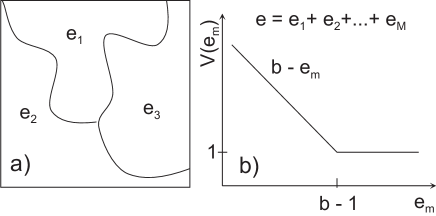
Figure 4: (a) The division of the total system in M independent subsystems (here: M=3). Of course, the borders are expected to fluctuate with time. (b) Every subsystem is described by a trap-model, which is characterized by the function $V(e)$.

In order to reproduce the thermodynamics of the BMLJ system the distribution of traps $G(e)$ in each subsystem has to be chosen as

$$G_{M}(e_{m})\propto\exp\left(-\frac{(e_{m}-(e_{0}/M))^{2}}{2(\sigma_{0}^{2}/M)}\right).$$ (6)

The dynamics is expected to strongly depend on the length scale of dynamic heterogeneities, i.e. on the value of $M$. In what follows, we will present results for different values of $M$ and identify the optimum choice.

As discussed above, the most relevant parameter of any trap model is the common barrier level $b$. For low energies this gives rise to the choice $V(e)=b-e$ as the barrier height to leave a trap (i.e. MB) of energy $e$. To cope with the high-energy limit of $V_{eff}(e)$, discussed above, we choose $V(e)=1.0$ for high $e$. The precise value is irrelevant for the results in the relevant temperature range. In total, we have $V(e)={\rm max}(b-e,1)$. This function is sketched in Fig.4b. The average waiting time in a trap of energy $e$ is given by

$$\tau(e,T)=\tau_{0}\exp(\beta V(e)).$$ (7)

The value of $\tau_{0}$ is a trivial scaling factor for the overall time scale and can be simply adjusted.

III.3 Dynamic interaction between subsystems

The ETM, introduced so far, starts from a collection of $M$ totally independent subsystems. However, one should rather expect that a local relaxation process may somewhat influence the state of the adjacent subsystems. Thus, some kind of dynamic interaction should be included, i.e. a modification of the state of an adjacent subsystem as a result of a relaxation process. In real space this modification might correspond to a minor shift of particles in the adjacent subsystems. This shift may somewhat change the probability for a relaxation process in these subsystems. Actually, already in the original paper of Monthus and Bouchaud their master equation for the energy probability distribution has been supplemented by an energy diffusion term which exactly takes into account the effect of relaxation processes on adjacent particles Monthus and Bouchaud (1996).

Here we introduce a simple ingredient of the ETM which reflects the relevant physics of the dynamic interaction. In particular we will take care that the thermodynamics of the total system is not modified. This condition is non-trivial because any variation of states may directly influence the probability distribution of states and thus change quantities like the average energy.

For the total system one may define the distribution $\varphi(e,T)$ via

$$\varphi(e,T)\propto p(e,T)/\langle\tau(e,T)\rangle.$$ (8)

It denotes the probability that after or before a transition a MB has the energy $e$. Thus, generation of MB according to the $\varphi(e)$-distribution (for convenience we suppress the dependence on T) yields the correct statistics of MB and thus the correct thermodynamics. Conceptually, the distribution $\varphi(e)$ is close to the distribution of MB, i.e. $G(e)$. Some minor (temperature dependent) deviations are present because in the present version of the trap model the relation $V(e)=b-e$ is not valid for the high-energy traps with $e>b-1$.

In what follows we generalize Eq.8 to the case $M>1$. First we consider the case $M=2$ but generalizations are straightforward. Let the subsystem 1 be in state $e_{1}$ and the subsystem 2 in state $e_{2}$. In the ETM the transition of the total system is achieved by a transition of one subensemble. Then the rate $1/\tau(e_{1},e_{2})$ for a transition of the system is given by the sum of the individual rates, i.e.

$$1/\tau(e_{1},e_{2})=1/\tau(e_{1})+1/\tau(e_{2}).$$ (9)

Furthermore due to the independence of the two subsystems the combined Boltzmann probability $p(e_{1},e_{2})$ is identical to the individual Boltzmann probabilities, i.e.

$$p(e_{1},e_{2})=p(e_{1})p(e_{2}).$$ (10)

Finally, the probability that after (or before) a transition of the total system one finds energies $e_{1}$ and $e_{2}$ is given by

$$\varphi(e_{1},e_{2}) \propto p(e_{1},e_{2})/\tau(e_{1},e_{2})$$ (11)

$$\propto p(e_{1})p(e_{2})(1/\tau(e_{1})+1/\tau(e_{2}))$$

$$\propto \varphi(e_{1})\tau(e_{1})\varphi(e_{2})\tau(e_{2})(1/\tau(e_{1})+1/\tau(e_{2}))$$

$$\propto \varphi(e_{1})\varphi(e_{2})(\tau(e_{1})+\tau(e_{2})).$$

Due to the enormous dynamic heterogeneities (see below) the waiting times are distributed over many orders of magnitude. Thus, at a randomly chosen time one will typically find both subsystems in traps of very different waiting times $\tau_{1}$ and $\tau_{2}$. Let us assume that a jump process occurred in subsystem 1. Then it is very likely that the state before the jump was characterized by $\tau_{1}\ll\tau_{2}$. Therefore one can write

$$\varphi(e_{1},e_{2})\propto\varphi(e_{1})\varphi(e_{2})\tau_{2}\propto\varphi(e_{1})p(e_{2}).$$ (12)

Now we may define the dynamic interaction. It is modelled such that after a jump in one subsystem with probability $q$ a new trap is selected in the other subsystem. According to Eq.12 the energy of the new trap in every subsystem has to be selected from the probability distribution $p(e_{2})$. This implies that the thermodynamics is not modified by the dynamic interaction. Furthermore, the principle of causality is directly implemented. Of course, in practice one would expect that every jump induces a minor rearrangement so that after $1/q$ jumps of the fast subsystem a total rearrangement with respect to the p-distribution has occurred. This gradual process, however, is very well approximated by the random process, introduced above.

Actually, for the low-energy limit, i.e. for $\tau(e_{2})\propto\exp(\beta(b-e_{2}))$, there exists a more intuitive rationalization of the factor $p(e_{2})$ in Eq.12. It is reasonable to assume that the probability for subsystem 2 to change its energy from $e_{2}^{\prime}$ to $e_{2}$ will be proportional to $\varphi(e_{2})$ and the Boltzmann factor $\exp(\beta(e_{2}^{\prime}-e_{2}))$. Therefore the probability to be in state $e_{2}$ is proportional to $\varphi(e_{2})\exp(\beta(e_{2}^{\prime}-e_{2})\propto\varphi(e_{2})\exp(-\beta e_{2})\propto\varphi(e_{2})\tau(e_{2})\propto p(e_{2})$. Of course, the original derivation of Eq.12 is more general.

For general $M$ one obtains the relation

$$\varphi(e_{1},...,e_{M})\propto\varphi(e_{1})p(e_{2})\cdot\cdot\cdot p(e_{M})$$ (13)

if a jump occurred in the first subsystem. Here we modify all subsystems $m=2,...,M$ with probability $q$ according to the respective Boltzmann distribution $p(e_{m})$. Evidently, in reality the dynamic interaction between subsystems may be somewhat more complicated. It will turn out, however, that this simple choice already captures the main effect of the interaction.

III.4 How to compare the ETM dynamics with the BMLJ dynamics?

So far we have introduced the ETM with three parameters $M$, $b$, and $q$. Every state is characterized by the internal parameters $e_{1},...,e_{M}$. The time evolution of the system according to the ETM is generated in a straightforward way. After a relaxation process in one of the $M$ subsystems a new energy is selected for this subsystem according to the $\varphi$-distribution, defined in Eq.8. Furthermore with probability $q$ a new energy is selected for the other $M-1$ subsystems according to the $p-distribution$, defined in Eq.4. The total energy of all subsystems is denoted $e^{i}$ (the upper index counts the number of transitions of the total system) . In the next step for every subsystem a waiting time $\tau_{act}(e_{m})$ is calculated. It is drawn from an exponential distribution with the average value $\tau(e_{m},T)$; see Eq.7. Then the subsystem with the shortest waiting time $\tau_{act,min}$ is selected to perform a relaxation process and the time proceeds by exactly $\tau^{i}\equiv\tau_{act,min}$. This procedure is then repeated and in the next step $e^{i+1}$ and $\tau^{i+1}$ are obtained etc. The output is a sequence of waiting times $\{\tau^{i}\}$ and corresponding energies $\{e^{i}\}$. Exactly these two sequences can be also obtained from analysis of the equilibrium BMLJ dynamics.

Both series together characterize in a detailed way how the system is exploring the PEL. They are to a large extent characterized by (i) the first and second moments of their respective distribution functions and (ii) by their correlation functions

$$f_{\mu}(n)\equiv\langle\mu_{n}\mu_{0}-\langle\mu\rangle^{2}\rangle/\langle(\mu-\langle\mu\rangle)^{2}\rangle.$$ (14)

The variable $n$ counts the number of MB transitions and $\mu\in\{\tau,e\}$. The denominator guarantees that $f_{\mu}(0)=1$. Basically, the $f_{\mu}(n)$ express to which degree the waiting times and the MB energies are correlated after $n$ MB transitions. Since the trap distribution in the ETM is chosen in order to reproduce the thermodynamics of the BMLJ system, the distribution of energies is naturally recovered. Thus the observables $\langle\tau\rangle$, $\langle\tau^{2}\rangle,f_{\tau}(n)$ and $f_{e}(n)$ may be taken for comparison. If the ETM is an appropriate model to characterize the PEL it should be possible to choose the model parameters $M,b$ and $q$ such that the BMLJ results of these observables are recovered for the relevant temperature regime between 0.45 and 0.6.

It is important to clarify the influence of the dynamic interaction parameter $q$ on the series of waiting times and energies, respectively. Since our procedure does not change the distribution $\varphi(e_{1},e_{2})$ (here for M=2) and since the waiting times are directly related to the energies, the distributions of waiting times and energies do not depend on $q$. In contrast, due to the additional variation of energies (and thus waiting times) one may expect that the decay of $f_{\mu}(n)$ becomes faster with increasing $q$. Thus, except for comparison of $f_{\mu}(n)$ we may choose $q=0$.

IV Results of the mapping

So far we have developed a minimum model for the PEL of a glass-forming system based on the trap model as the elementary unit. Now we compare the resulting ETM with the BMLJ system. As already mentioned this comparison involves the time series of waiting times as well as the time series of MB energies.

IV.1 Time series of waiting times

First, we analyse the autocorrelation function $f_{\tau}(n)$. The result for the BMLJ system is shown in Fig.5. Interestingly, it turns out that already after one step the new waiting time is basically uncorrelated to the old waiting time. This observation can be easily rationalized in terms of the ETM. From Eq. 12 (or Eq. 13 for general $M$) it follows that the new state of subsystem 1 will be drawn according to the distribution $\varphi(e_{1})$. Since $\varphi(e_{1})$ is peaked at much higher energies than $p(e_{2})$ it is very likely that also the next jump occurs in subsystem 1 (see below for a closer analysis of this effect). Since, however, two successive energies in subsystem 1 are uncorrelated (by definition) the same holds for the two successive waiting times for this subsystem. Since these waiting times determine the waiting time of the total system (because subsystem 2 is basically immobile) one may conclude that in general two successive waiting times of the total system are to a very good approximation uncorrelated. Of course, it can be checked explicitly (data not shown). This non-trivial prediction fully agrees with the MD data for the BMLJ system.

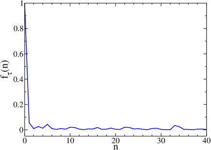
Figure 5: The correlation function of waiting times in dependence of the number of MB transitions for the BMLJ system at $T=0.5$.

Now we discuss the first and the second moment of the waiting time distribution $f(\tau)$ which, of course, strongly depends on temperature. As discussed above we may set $q=0$ for the comparison with the BMLJ system. In a first step we determine the respective values of $b$ (for different values of $M$) from the condition that the temperature dependence of $\langle\tau\rangle$ should agree as well as possible with the BMLJ data.

There are two different ways to estimate the value of $\langle\tau\rangle$. On the one hand, one can calculate the average of all waiting times, observed during a simulation run of time $t_{sim}$. On the other hand, one may determine the number of transitions $n$ and take $t_{sim}/n$ as the average waiting time. As shown in Appendix I the second choice can be applied for any simulation time $t_{sim}$. In contrast, the first choice is only applicable for very large $t_{sim}$. Therefore we prefer to use the second choice.

In Fig.6 we show the temperature dependence of the average waiting time $\langle\tau(T)\rangle$ as obtained from the MD simulations. These data are used to determine an optimum value of the common barrier level $b$ for the different choices of $M$. The resulting predictions for the ETM are also included in Fig.6. The values for $b$, obtained from this fitting, are listed in Tab.1. The agreement with the BMLJ data is not perfect but this single fitting parameter $b$ is enough to reproduce the temperature dependence in the relevant temperature range between 0.45 and 0.6 in a semi-quantitative way. By increasing the value of $b$ it would have been possible to improve the agreement for low temperatures whereas the deviations at higher temperatures would have become stronger. In any event, the temperature dependence of the ETM for the different values of $M$ looks very similar. Deviations at higher temperatures are expected because in this regime flow-like processes become more important which, of course, cannot be fully captured by the ETM.

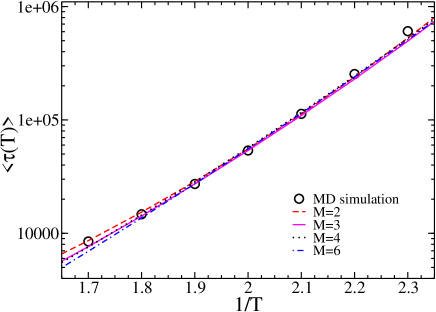
Figure 6: The average waiting time of MD simulations as compared with the predictions of the ETM with different values of $M$. The resulting values of $b$ and $\tau_{0}$ for the different $M$ are given in Tab.1.

M	b	$\tau_{0}$
2	-143.1	160
3	-93.3	43
4	-68.3	14
6	-43.4	4

Table 1: The values of the barrier level $b$ and the prefactor $\tau_{0}$, obtained from the fitting as discussed in Fig.6.

So far we have analyzed the average waiting time. At a given temperature it has contributions from MB with very different energies. Therefore it is more informative to analyze the waiting time in dependence of temperature and energy. As expressed by Eq. 5 there is a significant dependence of the average waiting time on the MB energy in the BMLJ system. For this purpose we consider the energy-dependence of the quantity $T\ln\langle\tau(e,T)\rangle$. For a simple trap model (see Eq. 7) it is linear with slope -1. What is the result for the ETM? The result for $M=3$ is shown in Fig.7a for the energy interval [-300,-295]. Interestingly, for all temperatures (T=0.45;T=0.5;T=0.6) a constant slope is observed which furthermore is identical for the three curves. For the energy interval $[-300,-295]$ the data for the different temperatures can thus be consistently described by

$$T\ln\langle\tau(e,T)\rangle\approx const(T)-ce$$ (15)

with $c=0.33$. We have repeated the same analysis for the different values of $M$. One observes the same behavior except for different values of $c$; see Tab.2.

Actually, the value of $c$ can be also estimated from general arguments which have been already partly presented in Doliwa and Heuer (2003a). For $M$ subsystems and individual energies $(e_{1},...,e_{M})$ in the limit of low temperatures the activation energy is given by min$[V(e_{1}),...V(e_{M})]=V(e_{max})$ where $e_{max}$ is the largest value of the $\{e_{m}\}$. To calculate the apparent activation energy $V_{eff}(e)$ for fixed total energy $e$, one has to average this expression over different realizations of the $e_{m}$ under the constraint $e=e_{1}+...+e_{M}$. As a first approximation, however, one may take $e_{max}\approx e/M+\Delta e$. The second term accounts for the deviation of $e_{max}$ from the average value $e/M$. It can be expected that $\Delta e$ only weakly depends on $e$. Then one has

$$V_{eff}(e)=V(e_{max})=V(e/M+\Delta e)\approx const-(1/M)e$$ (16)

Thus one expects that the slope $c$ is close to $1/M$ which is in excellent agreement with the numerical results in Tab.2.

In analogy to the ETM we have calculated the quantity $T\ln\langle\tau(e,T)\rangle$ for the BMLJ system for the same temperatures. The results are displayed in Fig.7b. Interestingly, the data also display a linear energy-dependence. Therefore it is possible to directly extract the value of $M$ if the BMLJ data are interpreted in terms of a ETM. For the two lowest temperatures the resulting slope is closest to $M=3$. For reasons of simplicity we also choose $M=3$ for the $T=0.6$. The weak temperature-dependence of the slope will be further discussed below. We note in passing that for a monatomic Lennard-Jones system of 32 particles the average barrier height linearly depends on energy with slope one. This would correspond to M=1 and is thus qualitatively compatible with the present result for a larger (and somewhat different) system Chowdhary and Keyes (2004).

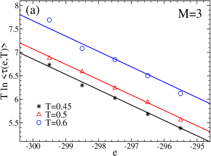
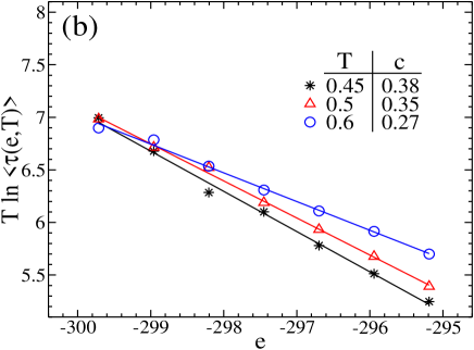
Figure 7: The quantity $T\ln\langle\tau(e,T)\rangle$ for different energies and temperatures in the energy range [-300,-295]. a) Results for the ETM for the example $M=3$. The resulting slopes for all relevant values of $M$ are listed in Tab.2. b) Results for the BMLJ. The resulting temperature-dependent slopes are included in the Figure.

M	c
2	0.44
3	0.33
4	0.25
6	0.17

Table 2: The slope $c$ obtained from analyzing the energy dependence of $T\ln\langle\tau(e,T)\rangle$ in Fig.7.

In the next step we want to elucidate the nature of the fluctuations. A natural choice would be the quantity

$$S(T)\equiv\frac{\langle\tau^{2}\rangle-\langle\tau\rangle^{2}}{\langle\tau\rangle^{2}}$$ (17)

including the first and the second moment of the waiting time distribution $f(\tau)$. It can be regarded as a measure for the normalized variance of the waiting time distribution. Around $T_{c}$ one approximately finds $f(\tau)\propto\tau^{-2}$ for large $\tau$. Without a cutoff of $f(\tau)$ at long times the variance would diverge for this distribution. This implies that the variance is extremely sensitive on the cutoff-behavior of $f(\tau)$. For temperatures around $T_{c}$ this cutoff can be predicted from Eq.7 by setting $\epsilon=-306$ as an estimate for the low-energy cutoff of the energy landscape. It turns out $\tau_{max}\approx 10^{5}\langle\tau\rangle$ which corresponds to roughly $10^{10}$ MD steps. Only for simulation times much longer than $\tau_{max}$ and thus many orders of magnitude longer than possible by present computer technology the variance of the observed waiting time distribution can be determined from simulations around $T_{c}$. This will be explicitly demonstrated in the next Section.

Evidently, the very long waiting times result from MB with very low energies. Therefore it may be very instructive to analyze the fluctuations of waiting times of MB, restricted to energy $e$. This restricted quantity is denoted as $S(e,T)$. For very low energies one may expect that due to the extremely small number of contributing MB the estimated variance will be smaller than the true variance. Only for higher energies $S(e,T)$ can be estimated without systematic errors from finite simulation times. We restrict ourselves again to the interval $[-300,-295]$. $S(e,T)$ is expected to show a sensitive dependence on the nature of the ETM. If, for example, the total BMLJ system could be described as a single trap system ($M=1$), MB with energy $e$ would be described by a single relaxation rate, yielding $S(e)=1$. For $M>1$ the total energy can be decomposed in different ways, resulting in different values of $\tau(e_{1},...,e_{M})$ for fixed total energy $e_{1}+...+e_{M}$; see Eq.9. The resulting distribution is a sum of different exponentially distributed functions, giving rise to $S(e)>1$. The data for the BMLJ system for $T=0.45;0.5;0.6$ are shown in the inset of Fig.8 for the interval $e\in[-300,-295]$. The average value of $S(e,T)$ in this interval is denoted $S_{0}(T)$. It is plotted in Fig.8 for the three temperatures. Furthermore we have added the predictions for $S_{0}(T)$ of the ETM for $M=3$ and $M=6$. It turns out that the data are inconsistent with the predictions of the ETM for $M=3$. Rather a good agreement with $M=6$ is suggested. As will be discussed further below a very natural mechanism may exist which reduces the size of the fluctuations of waiting times for a real system as compared to the predictions of the ETM. Therefore we propose that $M\approx 3$ as obtained from the analysis of $\langle\tau(e,T)\rangle$ is indeed the relevant value for the ETM.

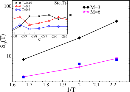
Figure 8: Inset: Energy-dependence of the normalized variance $S(e,T)$ for different temperatures for the BMLJ system. Main panel: Comparison of the respective average values $S_{0}(T)$ with the predictions of the ETM for $M=3$ and $M=6$.

IV.2 Sequence of energies

In a last step we analyse the sequence of MB energies. Since the energy distribution of the real system is naturally recovered by the trap model (see above) the non-trivial aspect is related to possible correlations of successive MB energies as measured by the autocorrelation function $f_{e}(n)$. The function $f_{e}(n)$, obtained for the BMLJ system, is shown in Fig.9. Since for $T=0.5$ one has $\tau_{\alpha}\approx 20\langle\tau\rangle$ ($\tau_{\alpha}$ determined from the incoherent scattering function) the energy correlation decays on the time scale of the $\alpha$-relaxation.

Dramatic differences are visible when comparing $f_{e}(n)$ with the predictions of the ETM (M=3)without including the dynamic interaction, i.e. $q=0$. Whereas the energies for the BMLJ system significantly decorrelate after 40 steps, basically no decorrelation is seen for the ETM. This can be easily rationalized. In the typical scenario, discussed above, very often there exists one subsystem which is much faster than the other two subsystems and, correspondingly, has a relatively high energy. This fast subsystem jumps and, on average, will acquire a new waiting time which is still much faster than the waiting time of the other two subsystems. Thus the energy of the slower systems will remain unchanged even after a large number of transitions. This automatically implies strong correlations for successive total energies of the ETM.

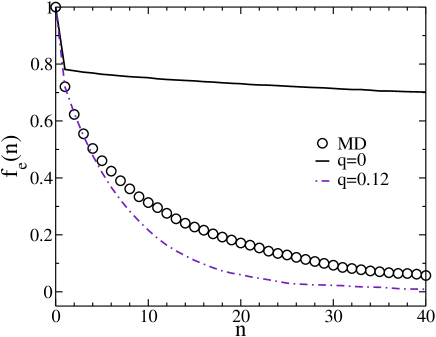
Figure 9: Decay of the energy-autocorrelation function in dependence of the number of MB transitions at T=0.5. Shown are the MD data for the BMLJ system (circles) and the predictions with ($q=0.12)$ and without ($q=0.0)$ dynamic coupling for the case $M=3$.

In contrast, a finite dynamic interaction results in additional reorganisation processes of the slow subsystems, thereby changing their energy according to the p-distribution. Although $p(e,T)$ is shifted to lower energies as compared to $\varphi(e,T)$ there will be the chance to acquire a relatively high energy after a few transitions of the fast subsystem and start to contribute to the relaxation. Therefore one can expect that a finite $q$ will give rise to a considerable decorrelation of energy. This can be seen in Fig.9 where data for $q=0.12$ are included. With this value the initial part of the decorrelation can be reproduced. Taking the strong dependence of $f_{e}(n)$ on the value of $q$ into account one may estimate the uncertainty of this value by $\pm 0.02$. Actually, a similar analysis for the two other temperatures yield $q$-values in the same interval although the data suggest a minor temperature-dependence ($q(T=0.6)\approx 0.14;q(T=0.45)\approx 0.11$).

Of course, this mechanism of dynamic interaction is far too simple to explain the complex coupling between different relaxation modes in supercooled liquids. In particular, it turns out that finally the decorrelation, generated by the dynamic interaction, is too strong. From a physical point of view one would expect that states with lower energies are less sensitive to fluctuations in the neighborhood than states with somewhat higher energies. This implies a dependence of the strength of the dynamic interaction on energy. Qualitatively, this property would explain the remaining deviations in Fig.9. Unfortunately, when introducing an energy-dependent $q$-value one would be forced to modify the simple rule based on Eq.13 in order to obtain the same thermodynamic properties. This is beyond the scope of the present work and would not yield any relevant new insight into the nature of the PEL of the BMLJ system.

V Discussion

V.1 Length scales and finite-size effects

Analysing the time series of waiting times the BMLJ system with 65 particles behaves to a first approximation as if it were a superposition of $M\approx 3$ independent subsystems. Each subsystem contains on average 20-25 particles. However, performing MD simulations with this very small number of particles (and periodic boundary conditions) one would observe strong finite size effects. Thus, it is not possible to perform simulations on the level of the elementary units of the ETM. In this sense it is impossible to see the elementary trap system directly. Rather the properties of the individual subsystems, mainly expressed by the value of the barrier $b$, have to be extracted from the superposition of at least 2-3 subsystems, corresponding to roughly 65 particles in real space. Why does a PEL of a BMLJ system with only 20 particles show significant finite size effects? First, the presence of dynamic interaction directly shows that the coupling among adjacent regions of the supercooled liquid is essential for the dynamics. Second, one can imagine that the real-space pattern of those particles which move together during one MB transition may be shaped in an string-like manner Donati et al. (1999); Perera and Harrowell (1999). Therefore the minimum size system without major finite size effects has to be larger than the elementary subsystem of the ETM. Otherwise the real-space patterns cannot be formed appropriately.

Of course, one could repeat the analysis also for larger systems. Evidently, larger values of $M$ would have been found. In any event, since a BMLJ system with $N=130$ particles behaves like a superposition of two systems with $N=65$ particles one would end up with a ETM which is a trivial extension of the present system.

V.2 How to rationalize the size of waiting time fluctuations at constant energy?

The only observable which did not agree with the predictions of the ETM was the second moment of the waiting time distribution. The fluctuations at constant energy as expressed by $S_{0}(T)$ are smaller than expected for $M=3$. Is there a simple physical picture which may reconcile these results?

Recently a detailed real-space analysis of the nature of the MB transition has been performed for the BMLJ system Vogel et al. (2004). In particular the number of particles, participating at such a transition, has been studied. This number can be quantified by the participation number

$$z=\sum_{i}\frac{dr_{i}}{dR}.$$ (18)

Here the sum is over all large particles of the binary Lennard-Jones system. $dr_{i}$ is the displacement of the i-th particle and $dR^{2}$ is the total squared displacement of all large particles. In case that only one particle is moving one has $z=1$, in case of identical movement of $n$ particles one gets $z=n$. It turns out that for different MB transitions the participation number $z$ can have very different values. The resulting distribution $p(z)$ has significant contributions between $z\approx 8$ and $z\approx 25$. Since the absolute numbers somewhat depend on the definition of $z$ Reinisch and Heuer (2004b) we mainly stress the width of $p(z)$ rather than the absolute numbers.

In the ETM, as introduced above, we have introduced $M$ identical subsystems. If this corresponded to the real world of BMLJ systems, one would expect a very narrow distribution $p(z)$. The width of $p(z)$ therefore implies that the assumption of identical subsystems cannot hold. In any event, it is natural to assume that at a given time the set of subsystems displays different sizes; see Fig.10 for a simple sketch.

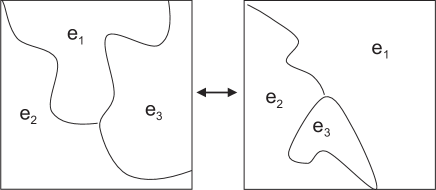
Figure 10: Sketch of the size fluctuations of a ETM with $M=3$.

To understand the effect of these fluctuations on the waiting time distribution one may consider the case of $M$ identical subsystems for fixed total energy $e$. The maximum waiting time of the total system is realized if by chance all $M$ subsystems have the energy $e/M$ and the corresponding waiting time $\tau_{e}$. Otherwise there is at least one subsystem with higher energy and (on average) shorter waiting time as compared to $\tau_{e}$. Thus the presence of the long-time wing of the waiting time distribution at constant energy is critically related to the presence of subsystems with identical waiting times. Allowing for size fluctuations it is likely that one subsystem is smaller than the other. Since on average smaller systems are faster than larger systems (see, e.g., Tab.2) one can expect that for a given total energy $e$ this subsystem and thus the total system has a waiting time much smaller than $\tau_{e}$. Therefore size fluctuations strongly reduce the probability to have a situation with a very long waiting time for the whole system. As a consequence, these fluctuations strongly suppress the long-time tail of the waiting time distribution, thereby reducing higher moments of this distribution. One may speculate that this is the reason that the fluctuations for the BMLJ are somewhat smaller than expected from the average waiting times. Of course, additionally also the value of $M$ may somewhat differ for different MB.

V.3 Implications for dynamic heterogeneities

The presence of short and long waiting times can be directly related to the concept of dynamic heterogeneities, observed in many experiments. As discussed above, a relevant measure for the presence of dynamic heterogeneities is the value of $S(T)$. On the level of the elementary subsystem in the ETM the dynamic heterogeneity is exclusively related to the presence of different trap depths which, via Eq.7, gives rise to a broad distribution of waiting times. For the BMLJ system with 65 or more particles, i.e. (in the language of the ETM) for a superposition of a few elementary subsystems, the dynamic heterogeneities can be formally divided into two parts. First, already at constant total energy $e$ one has a range of different waiting times as reflected by $S_{0}(T)>1$ (for $M>1$). Second, the average waiting time $\langle\tau(e,T)\rangle$ depends on energy. Comparing the size of $\sqrt{S_{0}(T=0.45)}\approx 3$ with the range of the energy dependence of $\langle\tau(e,T)\rangle$ it becomes obvious that for 65 particles the dynamic heterogeneities are mainly determined by the energy dependence of the average waiting time.

It is possible to characterize the properties of dynamic heterogeneities somewhat closer. As discussed before, the dynamic heterogeneities or, equivalently, the width of the waiting time distribution is captured by the normalized variance $S(T)$ (see Eq.17). In the limit of very long simulation times $t_{sim}$ as compared to the range of waiting times, the equilibrium value of $S(T)$ can be extracted from the simulations. How to find an appropriate way of extracting corresponding information at shorter simulation times? As already discussed in the context of the determination of $\langle\tau(T)\rangle$ it is convenient to analyse the number of MB transitions. Beyond the determination of the average number of MB transitions one can estimate its variance $\langle(n-\langle n\rangle)^{2}\rangle$ by comparing the number of MB transitions during a fixed time $t_{sim}$ of several independent simulations. Then one may define

$$S(T,t_{sim})=\frac{\langle(n-\langle n\rangle)^{2}\rangle}{\langle n\rangle^{2}}\frac{t_{sim}}{\langle\tau\rangle}.$$ (19)

As shown in Appendix II in the limit of long $t_{sim}$ the quantity $S(T,t_{sim})$ approaches the equilibrium value of $S(T)$. For shorter times $S(T,t_{sim})$ reflects the normalized variance of that part of the waiting time distribution which can be accessed on the time scale of the simulation $t_{sim}$. Thus any dependence of $S(T,t_{sim})$ on $t_{sim}$ indicates that the finite simulation time introduces an artificial cutoff for the waiting time distribution. As shown in Fig.11 for $T\leq 0.5$ the value of $S(T,t_{sim})$ for the BMLJ system still shows a strong increase for $t_{sim}\approx 1000\langle\tau\rangle\approx 20\tau_{\alpha}$ which already corresponds to relatively long simulation times.

It may instructive to compare the long-time limit of $S(T,t_{sim})$ for the BMLJ system with the predictions of the ETM. We have estimated the latter value by taking (using $M=3$) $S(T)\cdot[S_{0,BMLJ}(T)/S_{0,ETM}(T)]$. The second factor corrects for the fact that the actual dynamic heterogeneities of traps with identical energy are smaller than the predictions of the ETM; see Fig.8. The results are included in Fig.11. For the highest temperature $T=0.6$ the long-time limit of $S(T,t_{sim})$ can be reached for $t_{sim}\approx 1000\langle\tau\rangle$. Good agreement with the prediction of the ETM is observed. The large estimates of $S(T)$ within the ETM for the two lower temperatures reflect the broad dynamic heterogeneity at low temperatures. They only fully show up in the limit of very long simulation times.

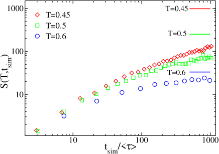
Figure 11: The dependence of the normalized variance $S(T,t_{sim})$ on simulation time $t_{sim}$ and temperature for the BMLJ system. The straight lines are the estimates of the ETM for the respective limiting values. The estimates for the ETM have been scaled by a factor, reflecting the deviations for $S_{0}(T)$ between the ETM and the BMLJ system.

This result has interesting consequences for the planning of simulations. The value of $S(T,t_{sim})$ is a measure how precisely the true value of $\langle\tau\rangle$ can be extracted from the simulation. More specifically, from $L$ independent runs the value of $\langle\tau\rangle$ can be extracted with a precision of $\sqrt{(S(T,t_{sim}))/(Lt_{sim}/\langle\tau\rangle)}$. Here we have assumed that a simulation of length $t_{sim}$ implies the drawing of $t_{sim}/\langle\tau\rangle$ independent waiting times. If $S(T,t_{sim})$ does not depend on $t_{sim}$ one could either perform a long simulation or several short simulations to obtain the same quality of $\langle\tau\rangle$. Due to the time-dependence of $S(T,t_{sim})$ it is more favorable to choose $t_{sim}$ relatively short and thus perform many independent runs for fixed total computer time. Alternatively, one can also perform a few simulations for a correspondingly larger system and obtain the same quality for the average waiting time. Since the diffusion constant is directly related to $\langle\tau\rangle$ the same conclusions hold for the determination of the diffusion constant.

Recently, the variance of the mean square displacement $\langle(r^{2}-\langle r^{2}\rangle)^{2}\rangle/\langle r^{2}\rangle^{2}$ has been obtained from comparison of independent simulation runs Nave and Sciortino (2004). On a superficial level this ratio resembles the quantity $\langle(n-\langle n\rangle)^{2}\rangle/\langle n\rangle^{2}$ analyzed above. A possible mapping between the observables $r^{2}$ and $n$ is further suggested by the validity of Eq. 1. Closer analysis, however, reveals that this mapping is not possible. For a simple random-walker in 1D one has $p(r^{2})dr^{2}=\exp(-r^{2}/\langle r^{2}\rangle)dr^{2}$ Nave and Sciortino (2004). In contrast, according to Appendix II the the value of $n$ displays a gaussian distribution around $\langle n\rangle$. As discussed in Nave and Sciortino (2004) the information content of the variance of the mean square displacement is more related to the size of dynamic heterogeneities whereas in the present case we are sensitive to the distribution of waiting times, i.e. to the degree of dynamic heterogeneities. In any event, the common idea is to use independent simulations to extract important information about the non-trivial dynamic properties of supercooled liquids.

Following the general ideas, underlying the Adam-Gibbs scenario or alternative descriptions of the physics of supercooled liquids at low temperatures Kirkpatrick et al. (1989); Xia and Wolynes (2001); Bouchaud and Biroli (2004) one might expect a growing length scale of the cooperativity range. In the present approach the length scale is reflected by the slope of $T\ln\langle\tau(e,T)\rangle$. Indeed, some temperature dependence has been observed, changing the slope by roughly 30 % when changing the temperature from $T_{c}$ (0.45) to $1.33T_{c}$ (0.6). In terms of the ETM this implies a weak temperature dependence of the cooperativity size. Actually, the slopes for $T=0.45$ and $T=0.5$ were compatible with $M=3$.

It may be instructive to compare this weak temperature dependence with that of other observables which characterize length scales of dynamic heterogeneities. Analogous behavior is observed for the average value of the participation number $z$; see Eq.18. This value is basically constant when comparing $T=0.5$ and $T=0.435$ Vogel et al. (2004). In contrast, a strong temperature-dependence is observed for quantities which are determined from the space-time behavior of particles. For example, the maximum of the generalized susceptibility , characterizing the size of cooperativity regions, varies by roughly a factor of 5 in the temperature regime analyzed in this work; see e.g. the behavior of $\chi_{M}$ in Ref.Glotzer et al. (2000). How to rationalize this apparent discrepancy? In the language of MB, dynamic heterogeneities have different facets: (i) The spatial range of particles moving during individual MB transitions. (ii) Spatial correlations of subsequent transitions Vogel et al. (2004). Both aspects are part of the ETM. The first aspect is directly reflected by the value of $M$. The second aspect is related to the question how many successive hops are on average performed by the same subsystem until a different subsystem relaxes. This value is denoted $n_{succ}$. It can be easily calculated from simulation of the ETM. As shown in Fig.12 $n_{succ}$ is strongly temperature-dependent and increases within the temperature regime of interest by a factor of 6. In the space-time analysis one is sensitive to the sequence of fast processes, i.e. the sequence of MB transitions. Thus one may expect that the increase of the generalized susceptibility with decreasing temperature is at least partly due to the increase of $n_{succ}$. On a qualitative level similar effects have been already reported in Vogel et al. (2004) where the formation of macro-strings out of micro-strings has been observed.

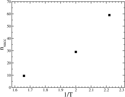
Figure 12: The average number $n_{succ}$ of successive hopping processes of the same subensemble in the ETM with $M=3$ for different temperatures.

VI Summary

Many observations for the BMLJ system are consistent with the notion that the PEL can be characterized as a superposition of individual trap-like systems where the individual traps are identified as MB (and not as inherent structures). The main observations are (i) the random-walk nature of the dynamics in phase space, (ii) the exponential waiting time distribution to leave MB, (iii) the temperature independent distance of subsequent MB, (iv) the absence of correlations of subsequent MB waiting times, and (v) the linear energy-dependence of $T\ln\langle\tau(e,T)\rangle$ for all temperatures. Analysis of the slightly temperature-dependent slope of $T\ln\langle\tau(e,T)\rangle$ yields information about the number $M$ of subsystems and the common barrier height $b$.

From the predictions of this simple model two deviations from the behavior of the BMLJ system have been observed. First, the energy correlation function decays faster than expected from the superposition of traps. This observation directly indicates the presence of some interaction between these subsystems, expressed by the dynamic interaction parameter $q$, thereby completing our definition of the extended trap model (ETM). Second, the dynamic heterogeneities of MB with constant $e$ were smaller than expected. This may be a natural consequence of size fluctuations of the subsystems. In principle it would be possible to include size fluctuations into the ETM by introducing a new parameter. This is, however, beyond the scope of the present work.

Our results may be helpful in several ways. The comparison of the BMLJ dynamics with the predictions of a superposition of appropriately chosen trap models may elucidate important properties of the PEL of a prototype glass-forming system. Furthermore, this analysis may serve as a fresh look onto the properties of dynamic heterogeneities. Finally, the ETM has the ability to reproduce also non-equilibrium properties at least on a semi-quantitative basis. For example it may be feasible to reproduce complex aging experiments and to obtain a simple physical picture of the resulting observations. For this purpose it is helpful that the relevant length scale for the ETM, as expressed by the value of $M$, is only weakly temperature dependent.

Appendix I

We consider a simple system which can be in different states with weights $\varphi_{i}$. The relaxation process in each state is characterized by an exponential waiting time distribution with average $\tau_{i}$. Thus the resulting average waiting time is given by $\langle\tau\rangle=\sum_{i}\varphi_{i}\tau_{i}$. In equilibrium the probability to be in state $i$ is given by $p_{i}=\varphi_{i}\tau_{i}/\langle\tau\rangle$. First, we consider a simulation of time $t_{sim}$ which is much smaller than any of the $\tau_{i}$. In particular one has $t_{sim}\ll\langle\tau\rangle$. The goal is to estimate the value of $\langle\tau\rangle$ from the outcome of the simulation. As described in the main text we may proceed in two different ways. One option is to determine the average waiting time. Since $t_{sim}$ is very small at most a single relaxation process will be observed. For calculating the average waiting time (in the ensemble average) the most convenient way would be to restrict oneself to those instances where at least a single relaxation process has occurred. Due to the smallness of $t_{sim}$ it may occur at any time with equal probability so that the average waiting time will be $t_{sim}/2$. This value is, of course, much smaller than the true average waiting time $\langle\tau\rangle$. Actually, only if $t_{sim}$ is much larger than all $\tau_{i}$ a consistent estimate is possible. The second option is to determine the average number $\langle n\rangle$ of relaxation processes. Weighting the initial state with its probability $p_{i}$, i.e. assuming equilibrium conditions, and taking into account that the chance of a relaxation process during time $t_{sim}$ is given by $t_{sim}/\tau_{i}$ one ends up with

$$\langle n\rangle=\sum_{i}p_{i}\frac{t_{sim}}{\tau_{i}}=\sum_{i}\varphi_{i}\frac{t_{sim}}{\langle\tau\rangle}=\frac{t_{sim}}{\langle\tau\rangle}.$$ (20)

Thus $t_{sim}/\langle n\rangle$ is an exact estimate of the average waiting time $\langle\tau\rangle$. This result also holds for larger values of $t_{sim}$ because the large time interval can be decomposed into small intervals and the average value of $\langle n\rangle$ will simply scale with the number of small time intervals such that $\langle n\rangle=t_{sim}/\langle\tau\rangle$ will hold for arbitrary $t_{sim}$.

Appendix II

Of conceptual interest is the variance $\sigma^{2}_{\tau}$ of the waiting time distribution. We show that it is related to the variance $\sigma^{2}_{n}$, obtained from a set of independent runs. According to the central limit theorem the probability that it takes a time $t$ to perform $n$ jumps is given by

$$p(t|n)\propto\exp\left(\frac{-(t-n\langle\tau\rangle)^{2}}{2n\sigma_{\tau}^{2}}\right).$$ (21)

Here we used that successive jumps are independent from each other so that we can consider a drawing of n independent elements from the waiting time distribution. Fixing the value of $t$ as $t_{sim}$ this probability can be reinterpreted as the probability $p(n|t)$ that exactly $n$ jumps occur during time $t_{sim}$. Thus one obtains

$$p(n|t_{sim})\propto\exp\left(\frac{-(n-t_{sim}/\langle\tau\rangle)^{2}}{2n\sigma_{\tau}^{2}/\langle\tau\rangle^{2}}\right).$$ (22)

In the limit of large $t_{sim}$ the n-dependence of the normalization factor can be neglected. Furthermore the factor $n$ in the denominator of the exponential can be substituted by $\langle n\rangle=t_{sim}/\langle\tau\rangle$. Therefore the variance of $n$, i.e. $\sigma_{n}$, can be written as

$$\frac{\sigma_{n}^{2}}{\langle n\rangle^{2}}=\frac{\sigma_{\tau}^{2}}{\langle\tau\rangle\langle n\rangle}=\frac{\langle\tau\rangle}{t_{sim}}\frac{\sigma_{\tau}^{2}}{\langle\tau\rangle^{2}}$$ (23)

This directly leads to Eq.19.