Dynamic Spin Structure Factor of SrCu₂(BO₃)₂ at Finite Temperatures

Abstract

Using finite temperature Lanczos technique on finite clusters we calculate dynamical spin structure factor of the quasi-two-dimensional dimer spin liquid SrCu₂(BO₃)₂ as a function of wavevector and temperature. Unusual temperature dependence of calculated spectra is in agreement with inelastic neutron scattering measurements. Normalized peak intensities of the single-triplet peak are ${\bf q}$-independent, their unusual temperature dependence is analyzed in terms of thermodynamic quantities.

I Introduction

In low-dimensional quantum spin systems quantum fluctuations often lead to disordered ground states that exhibit no magnetic ordering and a gapped, non-degenerate singlet ground state. Such states, also called spin liquids, are realized in one dimension in dimerised or frustrated spin chains, even-leg spin ladders as well as in the two dimensional Shastry-Sutherland (SHS) model.shastry81 SrCu₂(BO₃)₂ is a quasi-two-dimensional spin system with a unique spin-rotation invariant exchange topology that leads to a singlet dimer ground state. smith91 Since this compound represents the only known realization of the SHS model, it recently became a focal point of theoretical as well as experimental investigations in the field of frustrated spin systems. Consequently, many fascinating physical properties of SrCu₂(BO₃)₂ have been discovered. Increasing external magnetic field leads to a formation of magnetization plateaus kageyama99 ; onizuka00 which are a consequence of repulsive interaction between almost localized triplets. Weak anisotropic spin interactions can have disproportionately strong effect in a frustrated system. It has recently been shown, that the inclusion of the nearest neighbor (NN) and next-nearest neighbor (NNN) Dzyaloshinsky-Moriya (DM) interactions is required to explain some qualitative features of the specific heat near the transition from the spin dimer to the spin-triplet state, as well as to explain the low frequency lines observed in electron spin resonance experiments in SrCu₂(BO₃)₂. cepas01 ; cepas02 ; nojiri03 ; jorge03 ; zorko00 ; zorko01 ; elshawish

The existence of the spin gap, almost localized spin-triplet excited states, as well as the proximity of a spin-liquid ground state of SrCu₂(BO₃)₂ to the ordered antiferromagnetic state, lead to rather unusual low-temperature properties emerging in inelastic neutron scattering (INS),kageyama00 ; gaulin Raman scattering (RS) lemmens as well as in electron spin resonance (ESR) experiments. nojiri03 In particular, INS normalized peak intensities of single-, double- and possibly triple-modes show a rapid decrease with temperature around 13 K, well below the value of the spin gap energy $\Delta\sim 34$ K. In addition, authors of Ref. gaulin show, that properly normalized complement of static uniform spin susceptibility, obtained with almost identical model parameters as in the present work,jorge03 nearly perfectly fits their experimental data. Similar behavior is found in RS data where a dramatic decrease of Raman modes, representing transitions between the ground state and excited singlets, with increasing temperature at $T\ll\Delta$ is observed. Moreover, at $T\sim\Delta$ all RS modes become strongly overdamped.lemmens

Numerical simulations of dynamical spin structure factor based on exact diagonalization on small clusters at zero temperature show good agreement with INS data.miyahara03 Recently developed zero-temperature method based on perturbative continuous unitary transformations knetter ; knetter1 gives very reliable results for the dynamical spin structure factor of the SHS model since the method does not suffer from finite-size effects. The method is, however, limited to calculations at zero temperature and, at least at the present stage, it does not allow for the inclusion of DM terms.

The aim of this work is to investigate finite temperature properties of the dynamical spin structure factor of the SHS model using the finite temperature Lanczos method (FTLM),jj1 ; jj2 and to compare results with INS data.kageyama00 ; gaulin In our search for deeper physical understanding of spectral properties of the SHS model at finite temperatures we compare those with thermodynamic quantities, such as: the specific heat, entropy, and uniform static magnetic susceptibility, which we further compare with analytical results of the isolated dimer (DIM) model. We finally present results of the ${\bf q}$-dependent static magnetic susceptibility as a function of $T$.

II Model

To describe the low-temperature properties of SrCu₂(BO₃)₂ we consider the following Heisenberg Hamiltonian defined on a 2D Shastry-Sutherland lattice: shastry81

$$H_{s}\!\! = \!\!J\sum_{\langle{\bf i,j}\rangle}{\bf S_{i}\cdot S_{j}}+J^{\prime}\sum_{\langle{\bf i,j}\rangle^{\prime}}{\bf S_{i}\cdot S_{j}}$$ (1)

$$\,+ \!\!\sum_{\langle{\bf i\rightarrow j}\rangle^{\prime}}{\bf D^{\prime}}\cdot({\bf S_{i}\times S_{j}}).$$

Here, $\langle{{\bf i,j}}\rangle$ and $\langle{{\bf i,j}}\rangle^{\prime}$ indicate that ${\bf i}$ and ${\bf j}$ are NN and NNN, respectively. A recently published high-resolution INS measurments on SrCu₂(BO₃)₂ gaulin motivated us to choose $J=76.8$ K (in units of $k_{B}$) and $J^{\prime}/J=0.62$. A slightly different choice of parameters ($J=74.0$ K, $J^{\prime}/J=0.62$) has been used previously in describing specific heat measurements jorge03 and ESR experiments on SrCu₂(BO₃)₂.elshawish We should note, however, that this fine-tunning of parameters leads to effects, visible only on small energy scales, thus leaving previous calculations jorge03 ; elshawish practically unaffected. In addition to the Shastry-Sutherland Hamiltonian, $H_{s}$ includes DM interactions to NNN with the corresponding DM vector ${\bf D^{\prime}}$. The arrows indicate that bonds have a particular orientation as described in Ref. jorge03 . Its value, ${\bf D^{\prime}}=1.77\leavevmode\nobreak\ {\rm K}\leavevmode\nobreak\ {\hat{\bf z}}$, successfully explains the splitting between the two single-triplet excitations observed with ESR cepas01 ; nojiri03 and INS measurements.kageyama00 ; gaulin

As pointed out in Refs. jorge03 ; elshawish , a finite NN DM term should also be taken into account to explain specific heat data and ESR experiments. We have chosen to omit this term since it does not significantly affect results of the dynamical spin structure factor at a non-zero value of the wavevector. We have chosen the quantization axis $\hat{\bf z}$ to be parallel to the $c$-axis and $\hat{\bf x}$ to the $a$-axis pointing along the centers of neighboring parallel dimers.

We use the FTLM based on the Lanczos procedure of exact diagonalization, combined with random sampling over initial wave functions. For a detailed explaination of the method and a definition of method parameters see Refs. jj1 ; jj2 . All the results are computed on a tilted square lattice of $N=20$ sites with $M_{1}=100$ first and $M_{2}=250$ second Lanczos steps, respectively. The full trace summation over $N_{st}=2^{N}$ states is replaced by a much smaller set of $R\sim 500$ random states giving the sampling ratio $R/N_{st}\sim 5\cdot 10^{-4}$. Comparing FTLM with the conventional Quantum Monte Carlo (QMC) methods we emphasize the following advantages: (a) the absence of the minus-sign problem that usually hinders QMC calculations of frustrated spin systems, (b) the method connects the high- and low-temperature regimes in a continuous fashion, and (c) dynamic properties can be calculated straightforwardly in the real time in contrast to employing the analytical continuation from the imaginary time, necessary when using QMC calculations. Among the shortcomings of FTLM is its limitation to small lattices that leads to the appearance of finite-size effects as the temperature is lowered below a certain $T<T_{fs}$. Due to the existence of the gap in the excitation spectrum and the almost localized nature of the lowest triplet excitation, we estimate $T_{fs}\sim 1$ K at least for calculation of thermodynamic properties.jorge03 Finite-size effects also affect dynamical properties as, e.g., the dynamical spin structure factor, which is (even at finite temperatures) represented as a set of delta functions. In particular, finite-size effects affect the frequency resolution at low temperatures, while at higher temperatures as more states contribute to the spectra, its shape becomes less size dependent.

We should stress that FTLM was in the past successfully used in obtaining thermodynamic as well as dynamic properties of different correlated models as are: the $t$-$J$ model,jj1 ; jj2 the Hubbard model,bonca02 as well as the SHS model.jorge03

III Numerical Results and Comparison With Experiment

III.1 Dynamical Spin Structure Factor

For comparison with the INS data, we compute the dynamical spin structure factor for $\mu=x,y,z$

$$S_{\mu\mu}({\bf q},\omega)\!\! = \!\!{\rm Re}\int\limits_{0}^{\infty}\!\!dt\ e^{i\omega t}\left\langle S^{\mu}_{\bf q}(t)S^{\mu}_{\bf-q}(0)\right\rangle;$$

$$S^{\mu}_{\bf q}\!\! = \!\!\frac{1}{\sqrt{N}}\sum_{i,\alpha}S^{\mu}\left({\bf R}_{i}+{\bf r}_{\alpha}\right)e^{i{\bf q}\left({\bf R}_{i}+{\bf r}_{\alpha}\right)},$$ (2)

where $i$ runs over all unit cells of the lattice and ${\bf r}_{\alpha}$ spans four vectors forming the basis of the unit cell that contains two orthogonal dimers. For the details describing interatomic distances we refer the reader to Ref. knetter . The average in Eq. (2) represents the thermodynamic average which is computed using FTLM.jj1

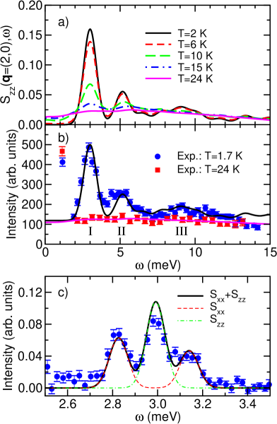
Figure 1: (Color online) (a) Spin structure factor $S_{zz}({\bf q},\omega)$ for ${\bf q}=(2,0)$ where ${\bf q}$ is given in units of the reciprocal lattice vectors defq vs. $\omega$ for different values of $T$, and (b) comparison with INS measurements from Ref. kageyama00 . Transitions to single-, double-, and triple-triplet states are indicated with Roman numerals. (c) Sum of the transverse $S_{yy}({\bf q},\omega)$ and longitudinal $S_{zz}({\bf q},\omega)$ contributions of a single-triplet mode compared to the high-resolution data for ${\bf q}=(-2,0)$ and $T=1.4$ K from Ref. gaulin . We use units where $\hbar=1$.

In Fig. 1(a) we first present the spin structure factor $S_{zz}({\bf q},\omega)$ for different temperatures. We should note that due to a finite value $D^{\prime}_{z}=1.77$ K spin rotational invariance of the Hamiltonian, Eq. (1), is broken, i.e. $S_{xx}({\bf q},\omega)=S_{yy}({\bf q},\omega)\neq S_{zz}({\bf q},\omega)$. Since $D^{\prime}_{z}\ll J,J^{\prime}$, the effect of broken symmetry is, at least within our numerical precision, negligible for energy resolutions much larger than the value of anisotropic interaction, $\Delta\omega\gg D^{\prime}_{z}$, yielding nearly identical results for the three components $\mu=x,y,$ and $z$ of $S_{\mu\mu}({\bf q},\omega)$. Since the spectra consist of a set of delta functions, we have artificially broadened the peaks with a Gaussian form with $\sigma=0.4$ meV, to achieve the best fit with INS measurements.kageyama00 Two peaks (I and II) are clearly visible at low temperatures $T=2\leavevmode\nobreak\ {\rm K}\ll\Delta$ around $\omega\sim 3$ meV and $5$ meV, associated with transitions to single- and double-triplet states. A broader peak (III) around $\omega=9$ meV represents transitions to triple-triplet states. Results at $T=2$ K are consistent with previous $T=0$ simulations. miyahara03 ; knetter Increasing temperature has a pronounced effect on $S_{zz}({\bf q},\omega)$, manifesting in a rapid decrease with temperature, at temperatures even far below the value of the gap. Quantitatively, at $T=24$ K the peak structure almost completely disappears. In Fig. 1(b) we present comparison of our numerical data scaled and shifted along the vertical axis to compensate for experimental background for two different temperatures along with experimental values from Ref. kageyama00 .

In order to investigate magnetic anisotropy effects one has to turn to high-energy resolution calculations with frequency precision comparable to the magnitude of the DM interaction. On this frequency scale we expect to find substancial difference between longitudinal and transverse components of the spin structure factor. For this reason we have included the transverse component of the spin structure factor according to the relation for the differential cross section

$$\frac{{\rm d}^{2}\sigma}{{\rm d}\Omega\,{\rm d}\omega}\propto\sum_{\mu\nu}\left(\delta_{\mu\nu}-\frac{q_{\mu}q_{\nu}}{q^{2}}\right)S_{\mu\nu}({\bf q},\omega).$$ (3)

For a given direction of the neutron momentum transfer, e.g., ${\bf q}=(-2,0)$ as used to obtain high-resolution INS data presented in Fig. 1(c), Eq. (3) reduces to a sum of the transverse and longitudinal part, ${{\rm d}^{2}\sigma}/{{\rm d}\Omega\,{\rm d}\omega}\propto S_{yy}({\bf q},\omega)+S_{zz}({\bf q},\omega)$. In Fig. 1(c) both contributions as well as their sum (Eq. (3)) are plotted against the high-resolution INS data.gaulin The best fit is achieved for $J=76.8$ K, $J^{\prime}=47.6$ K, $D^{\prime}_{z}=1.77$ K, and artificial broadening of the Gaussian form with $\sigma=0.05$ meV. The splitting $\Delta\sim 0.32$ meV between the outer two modes belonging to $S_{z}=\pm 1$ single-triplet excitations originates from a finite value $D^{\prime}_{z}$ yielding $4D^{\prime}_{z}/\Delta\sim 1.9$ for the renormalization of the bandwidth due to quantum fluctuations. This is as well in agreement with the estimate of Cepas et al.. cepas01

For comparison we also present $S_{zz}({\bf q},\omega)$ of the simplistic DIM model with $J=\Delta=34\leavevmode\nobreak\ {\rm K}$, where $J$ is chosen in such a way that SHS and DIM model share identical energy gaps between the singlet ground state and the excited triplet state. In the latter case analytical expression for $S_{zz}({\bf q},\omega)$ can be straightforwardly derived

$$S_{zz}({\bf q},\omega)\!\! = \!\!\pi A({\bf q})\left(\delta(\omega-J)+e^{-\beta J}\delta(\omega+J)\right)$$ (4)

$$\,+ \!2\pi B({\bf q})e^{-\beta J}\delta(\omega)$$

with $A({\bf q})$ and $B({\bf q})$ given by

$$A({\bf q})\!\! = \!\!\frac{\sin^{2}\eta(q_{x}-q_{y})+\sin^{2}\eta(q_{x}+q_{y})}{4(1+3e^{-\beta J})},$$ (5)

$$B({\bf q})\!\! = \!\!\frac{\cos^{2}\eta(q_{x}-q_{y})+\cos^{2}\eta(q_{x}+q_{y})}{4(1+3e^{-\beta J})},$$ (6)

and $\eta=0.717$. [Note also that in the limit $T\to\infty$ $\int_{-\infty}^{\infty}S_{zz}({\bf q},\omega)\,{\rm d}\omega=\pi/4$.] At $T=0$ $S_{zz}({\bf q},\omega)$ consists of a single delta function at $\omega=J$ weighted by $A({\bf q})$.kageyama00 This peak corresponds to peak I in the SHS model, while peaks II and III do not have their counterparts in $S_{zz}({\bf q},\omega)$ of the simplistic DIM model. With increasing $T$ peaks at $\omega=-J$ and $\omega=0$ appear, weighted by $\pi A({\bf q})\exp(-\beta J)$ and $2\pi B({\bf q})\exp(-\beta J)$, respectively.

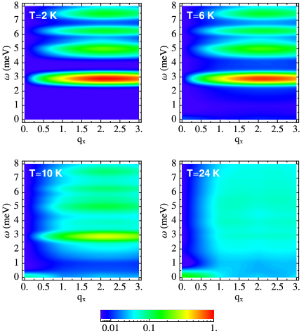
Figure 2: (Color online) Intensity plot of the spin structure factor $S_{zz}({\bf q},\omega)$ in the $q_{x}-\omega$ plane for different values of $T$ as indicated in the figures. The intensity scale is logarithmic and $\sigma=0.2$ meV is used to broaden the spectra as a function of frequency $\omega$. Note that due to the small system size only integer values of $q_{x}$ were numerically accesible.

In Fig. 2 we present a map of $S_{zz}({\bf q},\omega)$ for different temperatures. Peak I with almost no dispersion is clearly visible at $\omega\sim 3$ meV with its highest intensity located near $q_{x}\sim 2$. Peak II, located at $\omega\sim 5$ meV is also visible and similarly shows little dispersion. Its intensity is as well maximal near $q_{x}\sim 2$. Note that due to a small system size $S_{zz}({\bf q},\omega)$ plots were calculated at only a few discrete values of $q_{x}$, i.e., $q_{x}=0.0,1.0,2.0$ and 3.0. The geometry of the tilted square lattice with $N=20$ sites excludes half-integer values of $q_{x}$. This fact prevents us to directly compare our intensity plot results for the spin structure factor with the ones shown in Ref. gaulin , where the dispersion of the lowest triplet mode, attributed mainly to the transverse part of the spin structure factor, is clearly seen. We have calculated the transverse component $S_{yy}({\bf q},\omega)$ but since it does not differ considerably from $S_{zz}({\bf q},\omega)$ on a given energy scale we do not present it in Fig. 2. A final map, shown in Fig. 2, was obtained by interpolation between given integer values of $q_{x}$ points. These results are roughly consistent with measurements by Gaulin et al..gaulin With increasing $T$ peaks I and II rapidly decrease (more quantitative analysis of the temperature dependence follows in the next subsection), while visible response due to elastic transitions among identical multiplets starts developing around $\omega=0$ and $q_{x}=0$.

III.2 Normalized Peak Intensities

With the purpose to further quantify the agreement of our calculations with the experiment we present in Fig. 3 the normalized peak intensities $\tilde{I}/\tilde{I}_{0}$ of the two peaks (I and II) as functions of temperature along with the measured data taken from Ref. gaulin . To avoid contributions from the background at higher temperatures, peak intensities were measured from their values at $T=20$ K,

$$\tilde{I}/\tilde{I}_{0}=\frac{S_{zz}({\bf q},\omega_{P},T)-S_{zz}({\bf q},\omega_{P},20\leavevmode\nobreak\ {\rm K})}{S_{zz}({\bf q},\omega_{P},0)-S_{zz}({\bf q},\omega_{P},20\leavevmode\nobreak\ {\rm K})},$$ (7)

with $\omega_{P}=3.0$ meV and $\omega_{P}=5.0$ meV for peak I and II, respectively. Gaussian broadening with $\sigma=0.4$ meV was used to obtain peak values of $S_{zz}({\bf q},\omega_{P},T)$. A similar temperature behavior is observed as in INS measurements,gaulin ; kageyama00 manifesting itself in a rapid decrease of both peak intensities with temperature for $T$ far below the gap value $\Delta=34$ K. Taking this fact into account, the agreement between experimental values and numerical calculations of $\tilde{I}/\tilde{I}_{0}$ is reasonable even though not ideal. However, as already suggested by Gaulin et al.,gaulin nearly perfect agreement between experiment and rescaled complement of the uniform static susceptibility $1-\tilde{\chi}=1-\chi_{0}(T)/\chi_{0}(T=20\leavevmode\nobreak\ {\rm K})$ is found where $\chi_{0}=\langle{S^{z}_{tot}}^{2}\rangle/NT$, and $S^{z}_{tot}$ represents the $z$-component of the total spin. We were unable to find a direct analytical connection between the two quantities, i.e., $1-\tilde{\chi}$ and $\tilde{I}/\tilde{I}_{0}$, on the other hand the difference between the above mentioned quantities in numerical results are obvious from Fig. 3. Furthermore, analytical calculations of $1-\tilde{\chi}$ and $\tilde{I}/\tilde{I}_{0}$ on DIM model also indicate a different $T$ dependence. This leads us to the conclusion, that nearly perfect agreement with $1-\tilde{\chi}$ and experimental results of Ref. gaulin may be accidental.

In the inset of Fig. 3 we show the integrated intensities of the two peaks defined as $I(\omega_{1},\omega_{2})/I_{0}=\int_{\omega_{1}}^{\omega_{2}}{\rm d}\omega S_{zz}({\bf q},\omega)/\langle S_{\bf q}S_{-\bf q}\rangle$ where the limits of integration defining integrated peak intensities are defined as follows: $I_{I}=I(2\leavevmode\nobreak\ {\rm meV},4\leavevmode\nobreak\ {\rm meV})$ and $I_{II}=I(4\leavevmode\nobreak\ {\rm meV},6\leavevmode\nobreak\ {\rm meV})$ for peaks I and II, respectively. We observe a distinctive difference in temperature behavior between $I_{I}/I_{0}$ on the one hand and $I_{II}/I_{0}$ on the other. While $I_{I}/I_{0}$ substantially decreases with increasing temperature similarly to $\tilde{I}/\tilde{I}_{0}$, indicating on a considerable shift of the spectral weight away from transition I, $I_{II}/I_{0}$ shows even a slight temperature increase. We suggest that this difference is caused by a different nature of the transition from the ground state to the localized triplet (peak I) in contrast to transitions to states near or else within continuum (peak II). This behavior is as well in agreement with INS measurements kageyama00 that show peak I being only resolution limited while peaks II and III show intrinsic linewidths.

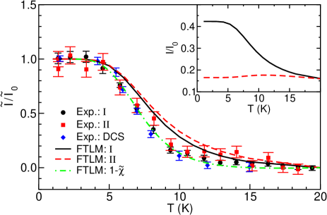
Figure 3: (Color online) Normalized peak intensities $\tilde{I}/\tilde{I}_{0}$ of peaks I and II vs. $T$ from Ref.gaulin (filled symbols), FTLM results (lines). The inset: relative integrated intensities $I/I_{0}$ of peaks I and II.

We now explore the ${\bf q}$-dependence of peak intensities. In Fig. 4 we present normalized values of peak intensities vs. $T$ for various values of $q_{x}$ at fixed $q_{y}=0$ and find nearly perfect scaling of $\tilde{I}/\tilde{I}_{0}$ for peak I, Fig. 4(a), while scaling breaks down at $q_{x}=3.0$ for peak II, Fig. 4(b). Such behavior is characteristic also for the simpler DIM model that possesses a single temperature scale $J$. This result suggests that a single temperature scale is responsible for the $T$ dependence of peak I for all different values of ${\bf q}$. In the insets of Figs. 4(a) and 4(b) we present absolute values of peak intensities for different values of $q_{x}$. Intensities of both peaks I and II reach their maximum values at low-$T$ near $q_{x}\sim 2.0$. Taking into account our rather poor resolution in the $q_{x}$-space, we find these results to be roughly consistent with recent high-resolution INS measurements by Gaulin et al..gaulin

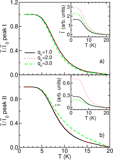
Figure 4: (Color online) Normalized peak intensities $\tilde{I}/\tilde{I}_{0}$ of peaks (a) I and (b) II vs. $T$ calculated at different values of ${\bf q}=(q_{x},0)$. In insets unrenormalized peak intensities measured from the peak intensity position at $T=20$ K are shown.

III.3 Thermodynamic Properties

Next, we will connect the spectral data with thermodynamic properties of the Hamiltonian defined in Eq. (1). For this reason we present in Fig. 5(a) the specific heat (per spin) $c=T(\partial s/\partial T)=(\langle H^{2}\rangle-\langle H\rangle^{2})/NT^{2}$ and the entropy density $s=lnZ/N+\langle H\rangle/NT$, where $Z$ is the statistical sum and $N$ is the number of spins in the system. Specific heat peaks around $T=T_{max}\sim 8$ K, where we also observe a rapid drop of $\tilde{I}/\tilde{I}_{0}$ [see Fig. 3], furthermore, this temperature also coincides with the steepest ascent of $s$. The peak in $c$, located well below the value of the gap, $T_{max}\sim 0.24\Delta$, is a consequence of excitations from the ground state to localized singlet and triplet states. This peak is followed by a broad shoulder above $T>15$ K which is due to excitations in the continuum. Note that $c$, obtained using the same method and for slightly different values of $J,J^{\prime}$ and ${\bf D}$, apart for additional DM terms, fits measured specific heat data of SrCu₂(BO₃)₂ in a wide range of applied external magnetic fields.jorge03 For comparison we also present $c$ and $s$ of the DIM model with $J=\Delta=34\leavevmode\nobreak\ {\rm K}$ that can be solved analytically. We should point out that even in a simple DIM model $c$ peaks well below the gap value, i.e., $T_{max}=0.35\Delta\sim 11.9$ K.

In Fig. 5(b) we present the uniform static spin susceptibility, $\chi_{0}=\langle{S^{z}_{tot}}^{2}\rangle/NT$, where $S^{z}_{tot}$ represents the $z$-component of the total spin. While comparison of $\chi_{0}$ with experimental data was presented elsewhere, jorge03 in this work we present it along with other thermodynamic properties just to gain a more complete physical picture of the temperature dependence of $S_{zz}({\bf q},\omega)$. The steepest increase in $\chi_{0}$ vs. $T$ coincides with the peak in $c$ and, at least approximately, with the steepest decreases of $\tilde{I}/\tilde{I}_{0}$, presented in Fig. 3. Due to the existence of the spin gap, $\chi_{0}(T\lesssim 5\leavevmode\nobreak\ {\rm K})\sim 0$, where the temperature interval $T\lesssim 5$ K in turn corresponds to the plateau of $\tilde{I}/\tilde{I}_{0}$ seen in experimental results of peaks I and II as well as in our numerical simulations.

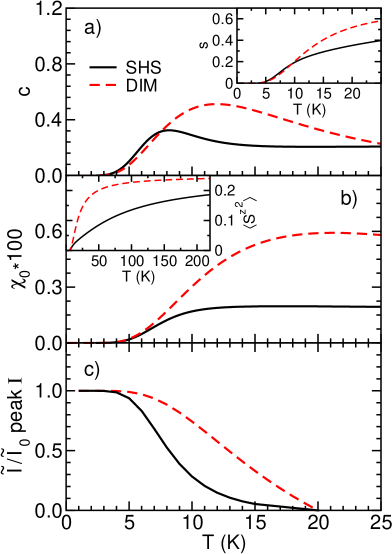
Figure 5: (Color online) Thermodynamic properties of the SHS model (full lines) and DIM model with $J=34\leavevmode\nobreak\ {\rm K}$ (dashed lines): (a) specific heat $c$ (entropy $s$ in the inset) vs. $T$ and (b) uniform static susceptibility $\chi_{0}$ vs. $T$. For completeness and to facilitate comparison we present in (c) normalized peak intensity of peak I $\tilde{I}/\tilde{I}_{0}$ vs. $T$ measured from values at $T=20$ K as shown in Fig. 3.

We would like to make some general remarks on comparing thermodynamic properties of the SHS model and the DIM model with identical gaps between the ground state and first excited states. Such a direct comparison may assist in understanding the influence of spin frustration and the proximity of gapless excitations in the SHS model on its thermodynamic properties. In particular, the specific heat $c$ of the SHS model peaks at lower temperature than $c$ of the DIM model and shows two maxima in contrast to a single, Schottky-like maximum seen in DIM model. The entropy of SHS model reveals slower increase with $T$ than that of the DIM model. And finally, the peak value of $\chi_{0}$ is almost three times lower in the SHS model than in the DIM model which in turn implies that spin fluctuations, $\langle{S^{z}}^{2}\rangle$, [see the inset of Fig. 5(b)] of the SHS model are suppressed in comparison to the DIM model.

III.4 Static Spin Susceptibility $\chi({\bf q})$

Finally, we present in Fig. 6 the static spin susceptibility

$$\chi({\bf q})\!\! = \!\!\frac{1}{\pi}{\cal P}\int\limits_{-\infty}^{\infty}\!\frac{\chi^{{}^{\prime\prime}}{(\bf q,\omega)}}{\omega}\ {\rm d}\omega,$$ (8)

$$\chi^{{}^{\prime\prime}}(\bf q,\omega)\!\! = \!\!\left(1-e^{-\beta\omega}\right)S_{zz}({\bf q},\omega),$$ (9)

as a function of ${\bf q}=(q_{x},0)$. Besides fulfilling theoretical interest, $\chi({\bf q})$ can also be used to compute, e.g., spin-spin nuclear relaxation rate $1/T_{2}$. Along $\chi({\bf q})$ of the SHS model we present for comparison results for the DIM model where analytical result can be readily obtained using Eqs. (4), (8), and (9):

$$\chi({\bf q})=2A({\bf q})\left(1-e^{-\beta J}\right)/J+2B({\bf q})e^{-\beta J}\beta$$ (10)

where $A({\bf q})$ and $B({\bf q})$ are defined in Eqs. (5) and (6). At low-$T$, i.e., $T\lesssim 5$ K, $\chi({\bf q})$ vs. $T$ is nearly $T$-independent which is a consequence of the spin gap. As a function of $q_{x}$ it reaches its maximum value near $q_{x}\sim 2.0$ in accord with the prediction of the DIM model result, Eq. (10). Observed $T$-dependence is again similar to the DIM model prediction. At higher temperatures, i.e., $T\gtrsim 300$ K, $\chi({\bf q})$ merges with universal, ${\bf q}$-independent form, i.e., $\chi({\bf q})=1/4T$.

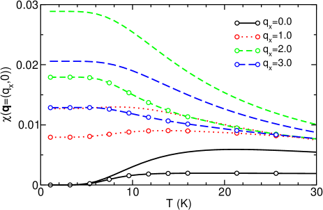
Figure 6: (Color online) $\chi({\bf q}=(q_{x},0))$ vs. $T$ for several values of $q_{x}$. Circles connected with lines present results of the SHS model, lines present results of the DIM model, Eq. (10) with $J=34$ K.

IV Conclusions

In conclusion, we have computed dynamical spin structure factor at finite temperatures. Frequency dependence of $S_{zz}({\bf q},\omega)$ at $T=2$ and 24 K agree reasonably well with INS measurements kageyama00 on a large energy scale despite rather poor frequency resolution caused by finite-size effects. High-resolution data for the lowest triplet excitation gaulin , on the other hand, is almost perfectly captured by calculated transverse and longitudinal components, $S_{yy}({\bf q},\omega)+S_{zz}({\bf q},\omega)$, showing the influence of anisotropy present in the system. Comparison of results obtained on systems with $N=16$ and 20 sites reveals that the positions of peaks I and II are reasonably well reproduced on $N=20$ system, while the peak III position and its structure are less accurate. We should also note that although in a 16-site system finite-size effects are somewhat more pronounced, this cluster enables one to calculate half-integer values of $q_{x}$ as well. By fitting the data from Ref. gaulin for all measured $q_{x}$ on a system with $N=16$ sites, we have concluded that additional NN in-plane as well as ’forbiden’ NN out-of-plane DM interactions are required to succesfully explain the structure and dispersion of peak I. However, the best fit is obtained with slightly different set of parameters as used in this work.

Temperature dependence of normalized peak intensities $\tilde{I}/\tilde{I}_{0}$ agrees well with INS measurements.kageyama00 ; gaulin Our calculations predict that $\tilde{I}/\tilde{I}_{0}$ of peak I should be ${\bf q}$-independent. Such behavior is in agreement with the DIM model prediction for peak I, while peak II is anyhow absent in this simplistic model. Our results are thus consistent with a proposition that a single temperature scale is responsible for the $T$ dependence of peak I for all different values of ${\bf q}$. This statement does not take into account a possible small dispersion of peak I due to DM interaction or (and) due to high-order processes in $J^{\prime}/J$. miyahara03 From comparison of temperature dependence of $\tilde{I}/\tilde{I}_{0}$ with thermodynamic properties it is obvious that strong $T$-dependence of $\tilde{I}/\tilde{I}_{0}$, occurring well below the value of the spin gap, is in accord with strong $T$-dependence of other thermodynamic properties. The temperature of the steepest decrease of $\tilde{I}/\tilde{I}_{0}$ coincides with the peak in $c$ and the steepest increase of $s$ as well as of $\chi_{0}$.

There is obviously a need for further, less finite-size dependent calculations that will clarify many unanswered questions as are, e.g., the role of DM terms in explaining small dispersion of peaks I and II observed in high-resolution INS experiments gaulin , an explanation of unusual temperature dependence of ESR lines nojiri03 that seem to decrease in width as the temperature increases, the occurrence of magnetization plateaus, etc. Nevertheless, the main features of temperature-dependent dynamic properties of the SHS model seem to be well captured by the FTLM on small lattices which is in turn reflected in a good agreement with experiments.

- (1) B. S. Shastry and B. Sutherland, Physica B 108, 1069 (1981).
- (2) R. W. Smith and D. A. Keszler, J. Solid State Chem. 93, 430 (1991).
- (3) H. Kageyama, K. Yoshimura, R. Stern, N. V. Mushnikov, K. Onizuka, M. Kato, K. Kosuge, C. P. Slichter, T. Goto, and Y. Ueda Phys. Rev. Lett. 82, 3168 (1999).
- (4) K. Onizuka, H. Kageyama, Y. Narumi, K. Kindo, Y. Ueda, and T. Goto, J. Phys. Soc. Jpn. 69, 1016 (2000).
- (5) O. Cépas, K. Kakurai, L. P. Regnault, T. Ziman, J. P. Boucher, N. Aso, M. Nishi, H. Kageyama, and Y. Ueda, Phys. Rev. Lett. 87, 167205 (2001).
- (6) O. Cépas, T. Sakai, and T. Ziman, Prog. Theor. Phys. Suppl. 145, 43 (2002).
- (7) H. Nojiri, H. Kageyama, Y. Ueda, and M. Motokawa, J. Phys. Soc. Jpn. 72, 3243 (2003).
- (8) G. A. Jorge, R. Stern, M. Jaime, N. Harrison, J. Bonča, S. El Shawish, C. D. Batista, H. A. Dabkowska, and B. D. Gaulin, Phys Rev. B 71, 092403 (2005).
- (9) A. Zorko, D. Arčon, H. Kageyama, and A. Lappas, Appl. Magn. Reson. 27, 267 (2004).
- (10) A. Zorko, D. Arčon, H. van Tol, L. C. Brunel, and H. Kageyama, Phys Rev. B 69, 174420 (2004).
- (11) S. El Shawish, J. Bonča, C. D. Batista, and I. Sega, Phys. Rev. B 71, 014413 (2005).
- (12) H. Kageyama, M. Nishi, N. Aso, K. Onizuka, T. Yosihama, K. Nukui, K. Kodama, K. Kakurai, and Y. Ueda, Phys. Rev. Lett. 84, 5876 (2000).
- (13) B. D. Gaulin, S. H. Lee, S. Haravifard, J. P. Castellan, A. J. Berlinsky, H. A. Dabkowska, Y. Qiu, and J. R. D. Copley Phys. Rev. Lett. 93, 267202 (2004).
- (14) P. Lemmens, M. Grove, M. Fischer, G. Güntherodt, Valeri N. Kotov, H. Kageyama, K. Onizuka, and Y. Ueda, Phys. Rev. Lett. 85, 2605 (2000).
- (15) S. Miyahara and K. Ueda, J. Phys.: Condens. Matter 15, R327 (2003).
- (16) Christian Knetter and Götz S. Uhrig, Phys. Rev. Lett. 92, 027204 (2004)
- (17) Kai P. Schmidt, Christian Knetter, and Götz S. Uhrig, Phys. Rev. B 69, 104417 (2004)
- (18) J. Jaklič and P. Prelovšek, Adv. Phys. 49, 1 (2000).
- (19) J. Jaklič and P. Prelovšek, Phys. Rev. Lett. 77, 892 (1996); Phys. Rev. B 49, 5065 (1994).
- (20) J. Bonča and P. Prelovšek, Phys. Rev. B 67, 085103 (2003).
- (21) Definition of the wavevector is identical to the one used in Refs. kageyama00 ; knetter .