Matter wave quantum dots (anti-dots) in ultracold atomic Bose-Fermi mixtures

Abstract

The properties of ultracold atomic Bose-Fermi mixtures in external potentials are investigated and the existence of gap solitons of Bose-Fermi mixtures in optical lattices demonstrated. Using a self-consistent approach we compute the energy spectrum and show that gap solitons can be viewed as matter wave realizations of quantum dots (anti-dots) with the bosonic density playing the role of trapping (expulsive) potential for the fermions. The fermionic states trapped in the condensate are shown to be at the bottom of the Fermi sea and therefore well protected from thermal decoherence. Energy levels, filling factors and parameters dependence of gap soliton quantum dots are also calculated both numerically and analytically.

I Introduction

The possibility to cool atomic Fermi gases below the Fermi temperature DeMarco with the developement of the sympathetic cooling technique Hulet has raised a significant amount of interest in theoretical and experimental studies of atomic Fermi gases embedded in Bose-Einstein condensates (BEC). Such systems have very interesting features which allow to explore a whole class of phenomena, ranging from strongly correlated effects in fermionic atomic gases to novel superfluid phases in Bose-Fermi mixtures (BFM) analogous to BCS superconductivity. The possibility to trap fermionic states into localized bosonic components of BFM makes these systems also of potential interest for quantum computing. The basic element of a quantum computer is the so called quantum bit, a special quantum state usually realized with a two-level system, which is manipulated by logical quantum gates (unitary operators) and which must be preserved intact for an extended period of time to allow computation Nielsen . An important role in this context is played by the interaction of the quantum system with the environment (thermal reservoir) which unavoidably produces decoherence. For an ideal q-bit one would like to keep the quantum system well protected from decoherence but not completely isolated from the environment to allow gate manipulations. This condition could be realized in Bose-Fermi mixtures by trapping fermionic states into localized BEC, so to form quantum dots with two (or more) fermionic levels inside, and by using Feshbach resonances to control the boson-fermion interaction, i.e. the coupling of the quantum bit with the environment.

The aim of this paper is twofold. From one side, we investigate the possibility of using ultracold Bose-Fermi mixtures to form matter wave quantum dots with two or more fermionic levels inside. To this regard we consider solitonic BEC states as trapping (expulsive) dot (antidot) potentials and show that the fermionic bound states formed inside are at the bottom of the Fermi sea and therefore well protected by thermal decoherence.

From the other side, we investigate the spectral properties of a BFM both in parabolic and in periodic potentials and demonstrate the existence of BFM gap-solitons in optical lattices (OL).

To this regard, we derive equations of motion for the mixture adopting a mean field approximation for the bosons and assuming non interacting (spin polarized) fermions in true quantum regime. These equations are solved by means of a self-consistent procedure and the spectral properties of BFM, both in parabolic traps and in optical lattices, derived. In particular, we show that fermionic bound state levels at the bottom of the Fermi sea can be trapped inside gap-solitons for both repulsive and attractive boson-boson interactions. We also show that, as the boson-fermion interaction is varied, the trapped levels undergo avoid crossings or level crossings according to the symmetry of the corresponding wavefunctions with respect to the OL. Analytical expressions for energy levels and for the number of fermionic bound states trapped inside attractive gap solitons are also derived and the results compared with those obtained from direct numerical self-consistent calculations. We find that the filling factor of a gap soliton follows the law $n_{f}\propto\sqrt{|\chi_{bf}|N_{b}}$, where $N_{b}$ is the number of bosons, $n_{f}$ the number of fermions trapped in the condensate and $\chi_{bf}$ the strength of the boson-fermion interaction. The possibility to change $\chi_{bf}$ in a wide interval of values using Feshbach resonances suggests the possibility of an experimental check of this results. In particular we expect that, as the boson-fermion interaction is increased, the progressive filling of the gap soliton should give rise to a depletion of fermions in the OL which follows the above law and which could be monitored by imaging techniques.

The paper is organized as follow. In section II we introduce the model and derive quasi-classical equation of motion of Bose-Fermi mixtures directly from a second quantized formulation of problem. In section III we investigate the energy spectrum for BFM in attractive and repulsive parabolic potentials and discuss quantum dots (antidots) analogies. In section IV we consider BFM in optical lattices and show the existence of gap solitons both for repulsive and attractive boson-boson interactions. The number of fermions trapped in a BFM gap soliton and the energies of the bound states are also calculated both numerically and analytically. Finally, in the last section the main results of the paper are briefly discussed and summarized.

II Equations of motion for a Bose-Fermi mixture

To derive equations of motion of a BFM it is convenient to start from the second quantized Hamiltonian of a set of bosons and fermions in interaction

$$\hat{H}=\int dr\hat{\psi}_{b}^{\dagger}(r)\hat{H}_{b}^{0}\hat{\psi}_{b}(r)+\int dr\hat{\psi}_{f}^{\dagger}(r)\hat{H}_{f}^{0}\hat{\psi}_{f}(r)+$$

$$\frac{1}{2}\int\int drdr^{\prime}\hat{\psi}_{b}^{\dagger}(r)\hat{\psi}_{b}^{\dagger}(r^{\prime})U_{bb}(r-r^{\prime})\hat{\psi}_{b}(r^{\prime})\hat{\psi}_{b}(r)+$$

$$\int\int drdr^{\prime}\hat{\psi}_{b}^{\dagger}(r)\hat{\psi}_{f}^{\dagger}(r^{\prime})U_{bf}(r-r^{\prime})\hat{\psi}_{b}(r^{\prime})\hat{\psi}_{f}(r),$$ (1)

where $\hat{H}_{b}^{0}=-\frac{\hbar^{2}}{2m_{b}}\nabla^{2}+V_{ext}^{b},\;\hat{H}_{f}^{0}=-\frac{\hbar^{2}}{2m_{f}}\nabla^{2}+V_{ext}^{f}$, are single particle hamiltonians accounting for the kinetic energy and for the external potential confining the bosons and the fermions, respectively, while $\hat{\psi}_{b}^{\dagger}(r),\hat{\psi}_{b}(r)$, $\hat{\psi}_{f}^{\dagger}(r),\hat{\psi}_{f}(r)$ are usual bosonic and fermionic field operators satisfying $[\hat{\psi}_{b}(r),\hat{\psi}_{b}(r^{\prime})]=[\hat{\psi}_{b}^{\dagger}(r),\hat{\psi}_{b}^{\dagger}(r^{\prime})]=0,\;[\hat{\psi}_{b}(r),\hat{\psi}_{b}^{\dagger}(r^{\prime})]=\delta(r-r^{\prime})$ (and similar relations for the fermionic fields with commutator replaced by the anti-commutator). Notice that the fermions are assumed spin polarized and therefore non interacting, so that only the boson-boson and boson-fermion interactions appear in the Hamiltonian. Using the above operator algebra, the Heisenberg equation of motion for the bosonic and fermionic fields can be written as

$$i\hbar\frac{\partial\hat{\psi}_{b}}{\partial t}=\hat{H}_{b}^{0}\hat{\psi}_{b}(r)+\int dr^{\prime}\hat{\psi}_{b}^{\dagger}(r^{\prime})U_{bb}(r-r^{\prime})\hat{\psi}_{b}(r^{\prime})\hat{\psi}_{b}(r)$$

$$+\int dr^{\prime}\hat{\psi}_{f}^{\dagger}(r^{\prime})U_{bf}(r-r^{\prime})\hat{\psi}_{f}(r^{\prime})\hat{\psi}_{b}(r),$$

$$i\hbar\frac{\partial\hat{\psi}_{f}}{\partial t}=\hat{H}_{f}^{0}\hat{\psi}_{f}(r)+\int dr^{\prime}\hat{\psi}_{b}^{\dagger}(r^{\prime})U_{bf}(r^{\prime}-r)\hat{\psi}_{f}(r^{\prime})\hat{\psi}_{f}(r).$$

For dilute mixtures one can replace the interaction potentials with the effective interactions

$$U_{bb}(r-r^{\prime})=g_{b}\delta(r-r^{\prime}),\;\;U_{bf}(r-r^{\prime})=g_{bf}\delta(r-r^{\prime}),$$ (2)

where the coupling constants $g_{b},g_{bf}$, are related to the s-wave scattering lengths $a_{b},a_{bf}$, by the relations: $g_{b}=4\pi\hbar^{2}a_{b}/m_{b}$, $g_{bf}=2\pi\hbar^{2}a_{bf}/m_{bf}$, where $m_{bf}$ denotes the reduced mass $m_{bf}=m_{b}m_{f}/(m_{b}+m_{f})$. Using these potentials, the above equations reduce to

$$i\hbar\frac{\partial\hat{\psi}_{b}(r,t)}{\partial t}=\left(\hat{H}_{b}^{0}+g_{b}\hat{\rho}_{b}(r,t)+g_{bf}\hat{\rho}_{f}(r,t)\right)\hat{\psi}_{b}(r),$$

$$i\hbar\frac{\partial\hat{\psi}_{f}(r,t)}{\partial t}=\left(\hat{H}_{f}^{0}+g_{bf}\hat{\rho}_{b}(r,t)\right)\hat{\psi}_{f}(r),$$ (3)

where $\hat{\rho}_{b}=\hat{\psi}_{b}^{\dagger}\hat{\psi}_{b}$ and $\hat{\rho}_{f}=\hat{\psi}_{f}^{\dagger}\hat{\psi}_{f}$, are the bosonic and fermionic particle densities, respectively. Expanding Bose and Fermi fields in terms of the usual creation and annihilation operators $\hat{a}^{\dagger},\hat{a}$ and $\hat{c}^{\dagger},\hat{c}$, for bosons and fermions, respectively,

$$\hat{\psi}_{b}(r,t)=\sum\psi^{b}_{n}\hat{a}_{n},\;\;\;\hat{\psi}_{f}(r,t)=\sum\psi^{f}_{n}\hat{c}_{n},$$

and replacing all field operators appearing in the bosonic equation with their expectation values on the ground state (mean field approximation)

$$\hat{\psi}_{b}\rightarrow\langle\hat{\psi}_{b}\rangle\approx\psi^{b}_{0}(r,t),\;\;\hat{\rho}_{b}\rightarrow\langle\hat{\rho}_{b}\rangle\approx N_{b}|\psi^{b}_{0}(r,t)|^{2},$$

$$\hat{\rho}_{f}\rightarrow\langle\hat{\rho}_{f}\rangle\approx\sum_{n=1}^{N_{f}}|\psi^{f}_{n}(r,t)|^{2},$$

we have that Eqs. (3) reduce to

$$i\hbar\frac{\partial\psi^{b}_{0}}{\partial t}=\left[\hat{H}_{b}^{0}+g_{b}N_{b}|\psi^{b}_{0}|^{2}+g_{bf}\left(\sum_{n=1}^{N_{f}}|\psi^{f}_{n}|^{2}\right)\right]\psi^{b}_{0},$$

$$\sum_{n}\left[i\hbar\frac{\partial\psi^{f}_{n}}{\partial t}-\hat{H}_{f}^{0}\psi^{f}_{n}-g_{bf}N_{b}|\psi^{b}_{0}|^{2}\psi^{f}_{n}\right]\hat{c}_{n}=0.$$ (4)

The completeness of the fermionic Fock space implies that the second equation in (4) can be satisfied only if the terms in the square bracket vanishes for all $n$ , this giving the following $N_{f}+1$ coupled equations

$$i\hbar\psi^{b}_{t}=\left[-\frac{\hbar^{2}}{2m_{b}}\nabla^{2}+V_{ext}^{b}+g_{b}N_{b}|\psi^{b}|^{2}+g_{bf}\rho_{f}\right]\psi^{b},$$

$$i\hbar\psi^{f}_{n_{t}}=\left[-\frac{\hbar^{2}}{2m_{f}}\nabla^{2}+V_{ext}^{f}+g_{bf}N_{b}|\psi^{b}|^{2}\right]\psi^{f}_{n},$$ (5)

with $\rho_{f}=\sum_{i=1}^{N_{f}}|\psi_{i}^{f}|^{2}$ the fermionic density and $\psi^{b}_{0}\equiv\psi^{b}$. From the above derivation it is clear that while bosons are treated in a classical mean field approximation the spin polarized fermions are in true quantum regime due to the lacking of interaction among them. Also note that for $g_{bf}=0$ the above equations separate into the Gross-Pitaevskii equation for the BEC part and $N_{f}$ identical (due to the lack of interaction among fermions) Schrödinger equations for the fermionic part of the mixture. Equations (5) were also derived in Karpiuk1 ; Karpiuk2 by means of a Lagrangian density approach.

In the following we shall consider Eq. (5) in a quasi one dimensional context by assuming the bosons and fermions confined in a cylindrical trap with transverse trapping frequency $\omega_{\perp}$ and negligible x-axial confinement. We also assume that the ground state energy of the transverse trapping potential $\hbar\omega_{\perp}$ is larger than the 3D ground state energies of the bosons and the fermions. Within this approximation the bosonic and fermionic wavefunctions can be factorized as $\psi=\psi(x)\psi_{\perp}(y,z)$ with the transverse wavefunction taken as the ground state of the trap potential independently of the longitudinal behavior and statistics das . By integrating over transverse coordinates one obtains effective 1D equations which are formally identical to Eqs. (5) but with boson-boson and boson-fermion interactions rescaled according to: $g_{b}\rightarrow 2\hbar\omega_{\perp}g_{b},\;\;\;g_{bf}\rightarrow 2\hbar\omega_{\perp}g_{bf}$.

Notice that the fact that fermionic and bosonic densities appear in the equations of bosons and fermions, respectively, suggests to consider them as effective potentials and solve the quasi-classical equation of motion by means of a self consistent procedure. Starting with a trial function for the bosonic part, we solve the quantum eigenvalue problems for the fermionic part, compute the fermionic density, derive the bosonic wavefunction by solving the bosonic equation and iterate the procedure until convergence is reached (an efficient implementation of this scheme for single BEC was discussed in salerno ). In the following we apply this method for BFM in parabolic traps and in optical lattices, concentrating, for simplicity, on the quasi one dimensional case.

III Bose-Fermi mixtures in a parabolic trap

In this section we consider BFM in a trap potential of the form $V_{trap}=\frac{\varepsilon}{2}m\omega^{2}(x-x_{0})^{2}$ and assume for simplicity $m_{b}=m_{f}$, $V_{ext}^{b}=V_{ext}^{f}=V_{trap}$ (the extension to the generic case is straightforward). We normalize Eqs. (5) by measuring space in harmonic oscillator length units $a_{0}=\sqrt{\hbar/m\omega}$, time in units of $\hbar/E_{0}$, with $E_{0}$ the zero point energy of the oscillator. Introducing the parameter $\chi_{b(bf)}$ as $g_{b(bf)}=(8\pi\hbar^{3}\omega_{\perp}a_{b_{0}(bf_{0})}/m)\chi_{b(bf)},\;$ where $a_{{b}_{0}},a_{{bf}_{0}}$ are scattering lengths in zero magnetic field (we use $\chi_{b(bf)}$ to change nonlinearities by means of external magnetic fields via Feshbach resonances), and rescaling wavefunctions according to $\psi^{b}\rightarrow(4\pi g_{{b}_{0}}N_{b}/m\omega a^{2}_{\perp})^{1/2}\psi^{b}$, $\psi^{f}\rightarrow(4\pi g_{{bf}_{0}}/m\omega a^{2}_{\perp})\psi^{f}$, with $a_{\perp}=(\hbar/m\omega_{\perp})^{1/2}$, we obtain the normalized equations

$$i\psi^{b}_{t}=-\psi^{b}_{xx}+V\psi^{b}+\chi_{b}|\psi^{b}|^{2}\psi^{b}+\chi_{bf}\rho_{f}\psi^{b},$$

$$i\hbar{\psi^{f}_{i}}_{t}=-{\psi^{f}_{i}}_{xx}+\left[V+\alpha\chi_{bf}|\psi^{b}|^{2}\right]\psi^{f}_{i},$$ (6)

where $V=\varepsilon(x-x_{0})^{2}$ and $\alpha=a_{bf}/a_{b}$ assumed in the following of the order of unity (notice that with this normalization the physical number of bosons $N_{p}$ is obtained from the dimensionless number $N_{b}$ as $N_{p}=m\omega a_{\perp}^{2}N_{b}/4\pi g_{{b}_{0}}$).

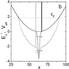
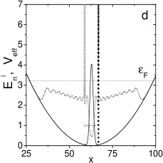
Figure 1: (a). Fermionic and bosonic densities for the case of $\chi_{b}=1,\chi_{bf}=-10$, $N_{f}=20$ and normalized number of bosons $N_{b}=1$, for a parabolic trap of strength $\varepsilon=0.0025$ centered at $x_{0}=L/2=20\pi$. (b) Effective potentials and energy levels of the Bose (open circles and dotted line) Fermi (filled circles and continuous line) mixture with densities given in panel(a) (horizontal line refers to the Fermi level). Panels (c) and (d) are the same as panels (a),(b), respectively, except for $\chi_{bf}=10$. Plotted quantities are in normalized units.

In Fig.1a we depict the bosonic and fermionic densities obtained with the self-consistent approach for a BFM with repulsive bosonic interactions ($\chi_{b}>0$) and attractive bosons fermion interaction ($\chi_{bf}<0$). We see that while the bosons remain confined in the middle of the trap, the fermionic density is quite extended in space and has a hump corresponding to the bosonic component. This hump originates from the contribution of the fermions trapped by the BEC acting on the fermions as a potential well (trapping impurity). Similar results were also reported in Karpiuk2 .

An interesting problem which has not been investigated is the distribution of the bosonic and fermionic levels in their effective potentials. This is done in Fig. 1b from which we see the presence of two fermionic levels formed below the parabola at the boottom of the Fermi sea. Notice that the effective potential seen by the fermions deviates from the original parabolic one only in the center of the trap due the presence of the potential well created by the bosonic density. Thus, the effective potential seen by the bosons is much deeper and wider, due to the contribution of the wide fermionic density and of their self-interaction. From this figure it is clear that two fermionic states have lowered their energies by adjusting themselves into the potential well created by the BEC giving rise in this way to a matter wave quantum dot i.e. a localized BEC with one or more fermionic levels trapped inside.

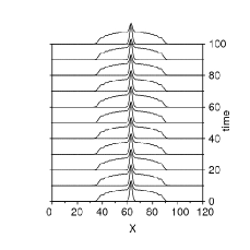
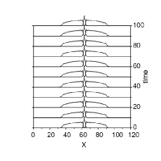
Figure 2: Time evolution of bosonic and fermionic densities in Fig. 1a (left panel) and Fig. 1c (right panel) obtained from the quasi-classical Eqs. (5) on a line of length $L=40\pi$. Space and time are in normalized units.

Notice that the two level system exists at the bottom of the Fermi sea and are separated by a gap from other fermionic levels which rapidly became equally spaced, as one would expect for a parabolic trap. Also notice that the ground state energy of the bosonic part of the mixture is lowered inside the potential well corresponding to the hump in the fermionic density and that excited states, although lowering their energies, remain almost equally spaced (this is due to the fact that the effective potential created by the fermions, except for the hump in the middle, looks still parabolic).

It is remarkable that this situation remains stable under time evolution, as one can see from the left panel of Fig. 2. In Fig. 1c, we show the situation for repulsive Bose-Fermi interactions ($\chi_{bf}>0$). From Fig. 1c we see that in this case fermions are expelled from (instead of attracted to) the region where bosons are spatially concentrated, this increasing their kinetic energy and rising a pressure on the condensate. Also notice from Fig. 1d that the corresponding energy levels are shifted up in energy, much more for bosons (which have an effective potential very deformed at the bottom) than for the fermions (which see almost the original parabolic trap but with a narrow hump in the middle). From this figure it is clear that the case of repulsive interactions ($\chi_{bf}>0$) is also of interest because, although not producing trapping states, it induces correlations among the fermions as is evident from the deviations from equally spaced levels observed in the region across the Fermi surface in Fig. 1d. This case can indeed be viewed as a matter wave anti-dot and could be used to investigate effects of strong correlations among fermions induced by the BEC .

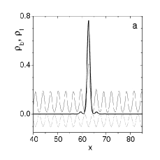
Figure 3: Panel (a). On-site symmetric densities for the case of $\chi_{b}=1,\chi_{bf}=-1$, $N_{f}=20$ and normalized number of bosons $N_{b}=1$ for an optical lattice of strength $\varepsilon=3$ (thick line refers to bosons). To identify the symmetry of the state the OL is reported with an amplitude scaled by a factor of $60$. Panel (b). Effective potentials (only lower part) and energy levels of the Bose (thin line and open circles) and Fermi (thick line and filled circles) mixture corresponding to the densities in panel(a). Lowest bosonic band (shadow region with negative slope) and lowest fermionic band (shadow region with positive slope) have also been shown. The fermionic band is half filled. Panels (c) and (d): the same as panels (a),(b), but for the inter-site symmetric case with $N_{b}=1.47$ . Plotted quantities are in normalized units.

IV Bose-Fermi mixtures in optical lattices

In this section we consider a trap potential of the form $V_{trap}=V_{0}\cos(2k_{L}x)$, as a model for an optical lattice. We assume $m_{b}=m_{f}=m$, $V_{ext}^{b}=V_{ext}^{f}=V_{trap}$ and normalize Eqs. (5) by measuring space in units of $k_{L}^{-1}$, time in units of $\hbar/E_{r}$ ($E_{r}=\hbar^{2}k_{L}^{2}/2m$ is the lattice recoil energy) and rescaling wavefunctions according to $\psi_{b}\rightarrow(g_{{b}_{0}}N_{b}/2\pi E_{r}{a_{\perp}}^{2})^{1/2}\psi_{b}$, $\psi_{f}\rightarrow(g_{{bf}_{0}}/2\pi E_{r}{a_{\perp}^{2}})^{1/2})^{1/2})\psi_{f}$. This leads to the same normalized equations (6) but with $V=\varepsilon\cos(2x)$, where $\varepsilon=V_{0}/E_{r}$. With this normalization the relation between the dimensionless number of bosons $N_{b}$ and the physical one is $N_{p}=(k_{L}a_{\perp}^{2}/a_{b})N_{b}$ (typical values are in the range of $10^{3}-10^{5}$ atoms, for $a_{\perp}\approx 10^{-6}m,k_{L}=10^{7}m^{-1},a_{b}=1\div 50\cdot 10^{-10}m$). In the following we show the existence of gap-solitons in BFM and suggest them as matter wave quantum dots (anti-dots) (the anti-dot case will be discussed elsewhere msalerno ).

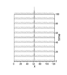
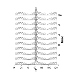
Figure 4: Time evolution of the OS (left panel) and IS (right panel) BFM densities in Fig. 3a and Fig. 3b obtained from direct numerical integrations of Eqs. (5) on a line of length $L=40\pi$. Space and time are in normalized units.

To this regard we consider BFM with repulsive bosonic-bosonic $\chi_{b}>0$ and attractive bosonic-fermionic $\chi_{bf}<0$ interactions. In Fig. 3a the bosonic and fermionic densities corresponding to an onsite symmetric (OS) gap soliton, are depicted (notice that the soliton is symmetric around a minimum of the potential). We see that while the bosonic density is localized in almost a single potential well, the fermionic density is very extended in space and presents a hump in correspondence of the BEC. In Fig. 3b the effective potentials, the sketch of the band structure and the energy levels of localized states for both bosons and fermions are shown. Notice that the energy of the OS gap soliton lies in the gap between the first two bands as expected for repulsive bosonic interactions, while the fermionic level responsible for the density hump in Fig. 3a, lies below the lowest energy band at the bottom of the Fermi sea. As for the parabolic case, gap soliton states with trapped fermionic levels inside can be seen a matter wave realization of quantum dots.

More complicated gap soliton states (or arrays of gap solitons) can also be formed. This is shown in Fig. 3c for the case of a two hump BEC condensate obtained as inter-site symmetric (IS) gap-soliton (notice that the state is symmetric around a maxima instead than a minima of the periodic potential). We see that also in this case the fermionic density increases in correspondence with the two bosonic humps and two fermionic levels are formed in the corresponding effective potential (see Fig. 3d). We have checked that both the OS and the IS modes are very stable under time evolution (see Fig. 4).

Gap- solitons with different symmetries with respect to the OL, such onsite-asymmetric (OA) and intersite-asymmetric (IA), can also exist in BFM but they appear to be metastable under time evolution. In Fig. 5a we show a gap-soliton of type IA together with two fermionic states trapped in the condensate. In panel (b) of this figure we depict the time evolution of the bosonic and fermionic densities of the IA gap-soliton as obtained from direct numerical integration of Eqs. (5).

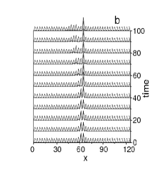
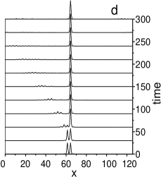
Figure 5: (a) Wavefunction of the intersite-asymmetric (IA) gap-soliton (thick line) plotted together with the wavefunctions of the lowest and first excited fermionic states trapped in the condensate (second and first curve from the top, respectively). The periodic potential, scaled by a factor 10 for graphical convenience, is also shown with a thin line at the bottom. Parameter values are the same as in Fig. 3 with $N_{b}=1$. (b) Time evolution of the bosonic and fermionic densities of the metastable IA gap-soliton obtained from the quasi-classical Eqs. (5) on a line of length $L=40\pi$. Panels (c). Same as panel (a) but for the OS state obtained after the transition. Panel (d). Time evolution of the wavefunction of the lowest energy state inside the condensate. Plotted quantities are in normalized units.

We see that after a time $t\approx 60$ the IA state decays into the stable OS wavefunction depicted in Fig. 5c. Notice that the IA-OS transition also induces changes in the fermionic states. In particular we see that the first excited state asymptotically decays into the Bloch state at the bottom of the fermionic band (see top curve of Fig.5c), while the lowest energy fermionic state remains well localized inside the gap soliton (see the time evolution reported in panel (c)). The IA-OS transition in Fig. 5c occurs therefore with the expulsion of one fermion from the condensate and with a change of symmetry of the wavefunction of the other fermion from IA to OS type (see second curves from the top in panels (a) and (c)). Similar phenomena occur for other metastable gap-solitons states existing in higher energy gaps and for different sign combinations of the interatomic interactions.

Also notice from Fig. 5b that the IA-OS transition occurs with emission of matter from the condensate meaning that the final OS gap soliton state contains less matter than the initial state. This implies that the corresponding effective potential for the fermions is weaker after the transition and therefore less effective to hold a second bound state in the condensate. As the boson-fermion (attractive) interaction and the number of bosons in the gap soliton are increased, we find that more fermionic levels are able to enter the condensate.

An interesting problem to investigate is how a matter wave q-dot (gap soliton) gets progressively filled with fermions as the product $\chi_{bf}N_{b}$ is increased. To this regard we consider OS bosonic gap solitons with attractive boson-fermion interaction and with both repulsive and attractive boson-boson interactions.

Figure 6: Left panel. Energy levels of the fermionic bound states inside the condensate as a function of $\chi_{bf}$, for parameter values $\chi_{b}=1,\varepsilon=3,N_{b}=1,N_{f}=20$. The top horizontal line represents the bottom of the fermionic band while the insets are enlargement of rectangles a,b, where level crossing and avoid crossing occur, respectively. Right Panel. Wavefunctions of the gap soliton (thick line) and of trapped fermionic states (ordered by decreasing energy from the top) at $\chi_{bf}=-30$. Other parameters are fixed as in the right panel. The vertical dotted line and the periodic potential at the bottom (scaled by a factor $60$) were drawn to identify the symmetry of the wavefunctions. A vertical offset among curves was introduced to avoid overlapping. All plotted quantities are in normalized units.

In the left panel of Fig. 6 we show the energy of the fermionic bound states inside the condensate as a function of $\chi_{bf}$ for the case of a repulsive BEC ($\chi_{b}>0$) with a fixed number of atoms. We see that the presence of an arbitrary small attraction between bosons and fermions is enough to trap at least one fermion in the gap soliton (notice that the energy of the fermion is below the edge of the lowest fermionic band, shown as a horizontal line in the figure). This is a consequence of the one dimensional nature of the effective potential (for BEC in higher dimensions a threshold in $\chi_{bf}$ is expected for the entering of the first fermion). From the inset (a) of the figure we see that two fermionic levels of almost equal energy enter the gap soliton at $\chi_{bf}\approx-3.5$. Notice that these levels come from extended (Bloch) states inside the fermionic band and are pulled below the lower band edge by the attractive boson-fermion interaction. The inset also shows that the two levels undergo a level crossing after which they proceed together as quasi degenerated states until a collision with a fourth level occurs. Notice that the last level detaches from the bottom of the fermionic band at $\chi_{bf}\approx-28.6$ and, in contrast with the previous case, it undergoes an avoid level crossing with the quasi degenerated states at $\chi_{bf}\approx-30$ (see inset (b)). Also notice that the avoid crossing occurs with an exchange of degeneracy, i.e. the newly entered level, originally non degenerate, becomes quasi degenerate after the interaction while the lowest energy level of the quasi degenerate pair becomes non degenerate after the interaction.

Figure 7: Bosonic density for attractive boson-boson interaction in an OL of strength $\varepsilon=0.5$. The continuous curve refers to the potential in Eq. 7 with $a=0.66$ while the dots represent self-consistent numerical results. Other parameters are fixed as $\chi_{b}=-1,\chi_{bf}=-10,N_{b}=4.9,N_{f}=20$. Right panel. Gap soliton (thick line) and trapped fermionic wavefunctions ordered by decreasing energy from the top. Parameters are fixed as in the left panel. The vertical dotted line and the periodic potential at the bottom (scaled by a factor of $4$) are drawn to identify the symmetry of the wavefunctions. A vertical offset among curves was introduced to avoid overlapping. All plotted quantities are in normalized units.

This behavior is in agreement with a general theorem of quantum mechanics, holding for hamiltonians depending on a parameter ( with eigenvalues functions of the parameter) according to which the level crossing occurs between levels of different symmetry and avoid crossing between states with the same symmetry. In the present case the wavefunctions of the fermionic levels inside the BEC can be either symmetric or asymmetric with respect to the OL site around which the gap soliton is centered. Moreover, the symmetry alternates between consecutive levels, the lowest state being always of OS type. This is seen from the right panel of Fig. 6 where we have depicted the gap soliton found at $\chi_{bf}=-30$ with the four fermionic states trapped inside. Notice that while the second and third bound states have different symmetries, and therefore their levels can cross, the second and fourth excited wavefunctions have the same symmetry and therefore their levels must give rise to an avoid crossing when approaching each other. This general rule for the crossing of the fermionic levels inside a gap soliton is in full agreement with the self-consistent numerical calculations shown in insets (a)-(b) of Fig. 6.

Analytical estimates for the energy levels and for the number of fermions in the condensate can be obtained for the case of an attractive BEC in shallow OL. To this regard we remark that for repulsive boson-boson interactions the bosonic density cannot be localized into a single potential well (due to the tunneling of matter into adjacent wells induced by the repulsive interaction), so that satellites around a main peak always appear (see the right panel of Fig. 6). In this case the corresponding effective potential in the fermionic Schrödinger equation gives rise to a spectral problem which is analytically difficult to solve. For attractive boson-boson interactions, however, the bosonic density may have no satellites peaks (due to the attraction) and can be easily approximated by integrable potentials (this is especially true when the OL is shallow).

In the following we consider the case of an attractive BEC with $\chi_{b}=-1$ in an OL of strength $\varepsilon=0.5$ and approximate the bosonic density with a Pöschl-Teller potential (soliton potential) of the form

$$\rho_{b}\approx\frac{N_{b}}{2a}\cosh^{-2}(\frac{x}{a}).$$ (7)

Notice that with this parametrization the condition $\int\rho_{b}dx=N_{b}$ is always satisfied so that $a$ can be used as a fit parameter. In the left panel of Fig. 7 we have compared the bosonic density obtained using the self-consistent method with the Pöschl-Teller approximation in Eq. (7), from which we see that the approximation is indeed quite good. The right panel of the figure shows the gap soliton with four trapped fermionic levels inside. Comparing these wavefunctions with the ones in Fig. 6 we see that, although different, they have the same symmetry properties with respect to the optical lattice. The fact that the bosonic density can be well approximated by a Pöschl-Teller potential allows to solve exactly the Schrödinger equation for the effective potential $V_{eff}=-|\chi_{bf}|\rho_{b}$ in terms of hypergeometric functions landau . The vanishing of bound state wavefunctions at large distances requires that the hypergeometric series must be reduced to a polynomial, this leading to the following analytical expression for the fermionic levels inside the condensate

$$E_{n}=-\frac{1}{4a^{2}}\left(2n+1-\sqrt{1+2a|\chi_{bf}|N_{b}}\right)^{2},n=0,1,...,n_{f}.$$ (8)

The number of discrete levels $n_{f}$ in the gap soliton is then obtained as the largest integer $n$ satisfying the inequality

$$n<\frac{1}{2}(\sqrt{1+2a|\chi_{bf}|N_{b}}-1).$$ (9)

In Fig. 8 we compare the energy levels obtained with the self-consistent method with those obtained from Eq. (8), from which we see that the agreement is quite good. In the right panel a similar comparison is made for the number of fermions $n_{f}$ versus $\chi_{bf}$, this further confirming the validity of our approximation. Notice that for $N_{b}|\chi_{bf}|a\gg 1$ the energy levels (8) coincide with those obtained with the WKB approximation valid for $n$ very large (in this limit $n_{f}$ can be approximated as $n_{f}\approx\sqrt{N_{b}|\chi_{bf}|a/2})$. From this we conclude that the number of fermionic levels at the bottom of the Fermi sea which can be trapped in a gap soliton can be controlled by changing the boson-fermion scattering length using Feshbach resonances.

Figure 8: Left panel. Energy levels of the fermionic bound states trapped inside an attractive condensate as a function of $\chi_{bf}$. The continuous curves refer to numerical results obtained with the self-consistent method while the dotted lines to the analytical expression in Eq. (8) with $a=0.66$ and $n=0,1,...,6$, from right to the left, respectively. The top horizontal line represents the bottom of the fermionic band. Parameters are fixed as in Fig. 7. Right panel. Number of fermions entering the gap soliton as a function of $\chi_{bf}$. The continuous curve refers to Eq. (9) with fitting parameter $a=0.66$. To account for the existence of one bound state at small $\chi_{bf}$ the curve has been shifted upward by $a$. All plotted quantities are in normalized units.

V Conclusions

In conclusion, we have shown that localized states of BFM with attractive (repulsive) Bose-Fermi interactions can be viewed as a matter wave realization of quantum dots (antidots). The case of BFM in optical lattices has been investigated in detail and the existence of gap solitons has been shown. In particular, we showed that gap-solitons can trap a number of fermionic bound state levels inside both for repulsive and attractive boson-boson interactions. These solutions may have different symmetries with respect to the OL and exist for a wide range of parameters. Gap solitons of BFM with OS and IA type are very stable under time evolution. We have shown that, as the boson-fermion interaction is changed the trapped fermionic levels inside the condensate may undergo level crossings or avoid crossings depending on the symmetry of the corresponding wavefunctions with respect to the optical lattice. This behavior is in agreement with a general theorem of quantum mechanics and shows that trapped fermions in BEC are in true quantum regime. The dependence of the number of bound states and of their energies on $N_{b}$ and $\chi_{bf}$ has been calculated both numerically and analytically. In particular, for attractive boson-boson interactions we approximated the bosonic density with a Pöschl-Teller potential and showed that a gap soliton in a shallow OL gives rise to a matter q-dot with filling number $n_{f}\propto\sqrt{|\chi_{bf}|N_{b}}$. The possibility to change the boson-fermion interaction in a large interval of values (both negative to positive) by means of a Feshbach resonance, makes the filling dependence of a matter q-dot on $\chi_{bf}$ experimentally feasible to check. To this regard we expect that as the (negative) boson-fermion scattering length is decreased, the progressive filling of the gap soliton gives rise to a depletion of fermions in the OL which follow the above law and which could be in principle monitored by imaging techniques. To this regard we remark that the existence of gap-solitons in one dimensional Bose-Einstein condensates in optical lattices has been experimentally demonstrated in Ref.markus . We believe that similar experiments can be performed also for Bose-Fermi mixtures in OL and we expect that gap solitons will be found also in this case.

Finally, we remark that the possibility to use gap solitons of BFM as q-bits protected from thermal dechoerence is very appealing and deserves further investigations.

Acknowledgments

Interesting discussions with F.Kh. Abdullaev and B.B. Baizakov are gratefully acknowledged. Financial support from the MURST-PRIN-2003 project Dynamical properties of Bose-Einstein condensates in optical lattices is also acknowledged.

References

- (1) B.DeMarco and D.S. Jin , Science 285, 1703 (1999)
- (2) A.G. Truscott, et al., Science 291, 2570 (2001); F.Schreck et al., Phys. Rev. Lett. 87, 080403 (2001); Z.Hadzibabic et al., ibid. 88, 160401 (2002); G.Roati, F.Riboli, G.Modugno, and M. Inguscio, ibid. 89, 150403 (2002);
- (3) see for example M.A. Nielsen and I.L.Chuang Quantum Computation and Quantum Information, Cambridge Univ. Press., Cambridge UK (2000).
- (4) T.Karpiuk et al.,Phys. Rev. A 69, 043603 (2004).
- (5) T.Karpiuk et al.,Phys. Rev. Lett. 93, 100401 (2004).
- (6) K.K. Das ,Phys. Rev. Lett. 90, 170403 (2003).
- (7) Mario Salerno, Laser Physics 15, 620 (2005); see also cond-mat/0311630.
- (8) Mario Salerno, (in preparation).
- (9) L.D.Landau, E.M. Lifshitz, Quantum Mechanics, Pergamon, 1977.
- (10) B. Eiermann et al., Phys. Rev. Lett. 92, 230401 (2004).