Self-similarity of complex networks

Abstract

Complex networks have been studied extensively due to their relevance to many real systems as diverse as the World-Wide-Web (WWW), the Internet, energy landscapes, biological and social networks ab-review ; mendes ; vespignani ; newman ; amaral . A large number of real networks are called “scale-free” because they show a power-law distribution of the number of links per node ab-review ; barabasi1999 ; faloutsos . However, it is widely believed that complex networks are not length-scale invariant or self-similar. This conclusion originates from the “small-world” property of these networks, which implies that the number of nodes increases exponentially with the “diameter” of the network erdos ; bollobas ; milgram ; watts , rather than the power-law relation expected for a self-similar structure. Nevertheless, here we present a novel approach to the analysis of such networks, revealing that their structure is indeed self-similar. This result is achieved by the application of a renormalization procedure which coarse-grains the system into boxes containing nodes within a given ”size”. Concurrently, we identify a power-law relation between the number of boxes needed to cover the network and the size of the box defining a finite self-similar exponent. These fundamental properties, which are shown for the WWW, social, cellular and protein-protein interaction networks, help to understand the emergence of the scale-free property in complex networks. They suggest a common self-organization dynamics of diverse networks at different scales into a critical state and in turn bring together previously unrelated fields: the statistical physics of complex networks with renormalization group, fractals and critical phenomena.

Two fundamental properties of real complex networks have attracted much attention recently: the small-world and the scale-free properties. Many naturally occurring networks are small world since one can reach a given node from another one, following the path with the smallest number of links between the nodes, in a very small number of steps. This corresponds to the so-called “six degrees of separation” in social networks milgram . It is mathematically expressed by the slow (logarithmic) increase of the average diameter of the network, $\bar{\ell}$, with the total number of nodes $N$, $\bar{\ell}\sim\ln N$, where $\ell$ is the shortest distance between two nodes and defines the distance metric in complex networks erdos ; bollobas ; watts ; barabasi1999 . Equivalently, we obtain:

$$N\sim e^{\bar{\ell}/\ell_{0}},$$ (1)

where $\ell_{0}$ is a characteristic length.

A second fundamental property in the study of complex networks arises with the discovery that the probability distribution of the number of links per node, $P(k)$ (also known as the degree distribution), can be represented by a power-law (scale-free) with a degree exponent $\gamma$ usually in the range $2<\gamma<3$ barabasi1999 ,

$$P(k)\sim k^{-\gamma}.$$ (2)

These discoveries have been confirmed in many empirical studies of diverse networks ab-review ; mendes ; vespignani ; newman ; barabasi1999 ; faloutsos .

With the aim of providing a deeper understanding of the underlying mechanism which leads to these common features one needs to probe the patterns within the network structure in more detail. The question of connectivity between groups of interconnected nodes on different length-scales has received less attention. Yet, a plethora of examples in Nature exhibits the importance of collective behavior, from interactions between communities within social networks, links between clusters of web-sites of similar subjects, all the way to the highly modular manner in which molecules interact to keep a cell alive. Here we show that real complex networks, such as WWW, social, protein-protein interaction networks (PIN) and cellular networks are indeed constructed of self-repeating patterns on all length-scales, and are therefore invariant or self-similar under a length-scale transformation.

This result comes as a surprise since the exponential increase in Eq. (1) has led to the general understanding that complex networks are not self-similar, since self-similarity requires a power-law relation between $N$ and $\ell$.

How can one reconcile the exponential increase in Eq. (1) with self-similarity, or in other words an underlying length-scale-invariant topology? At the root of the self-similar properties that we unravel in this study is a scale-invariant renormalization procedure which we show to be valid for dissimilar complex networks.

In order to demonstrate this concept we first consider a self-similar network embedded in Euclidean space, of which a classical example would be a fractal percolation cluster at criticality bunde-havlin . In order to unfold the self-similar properties of such clusters we calculate the fractal dimension using a “box counting” method and a “cluster growing” method vicsek .

In the first method we cover the percolation cluster with $N_{B}$ boxes of linear size $\ell_{B}$. The fractal dimension or box dimension $d_{B}$ is then given by feder :

$$N_{B}\sim\ell_{B}^{-d_{B}},$$ (3)

In the second method, the network is not covered with boxes, instead one seed node is chosen at random and a cluster of nodes centered at the seed and separated by a minimum distance $\ell$ is calculated. The procedure is then repeated by choosing many seed nodes at random and the average “mass” of the resulting clusters ($\langle M_{c}\rangle$, defined as the number of nodes in the cluster) is calculated as a function of $\ell$ to obtain the following scaling:

$$\langle M_{c}\rangle\sim\ell^{d_{f}},$$ (4)

defining the fractal cluster dimension $d_{f}$ feder . Comparing Eq. (4) and (1) implies that $d_{f}=\infty$ for complex small-world networks.

For a homogeneous network characterized by a narrow degree distribution (such as a fractal percolation cluster) the box covering method of Eq. (3) and the cluster growing method of Eq. (4) are equivalent since every node typically has the same number of links or neighbors. Equation (4) can then be derived from (3) and $d_{B}=d_{f}$, and this relation has been regularly used.

The crux of the matter is to understand how one can calculate a self-similar exponent (analogous to the fractal dimension in Euclidean space) in complex inhomogeneous networks with a broad degree distribution such as Eq. (2). Under these conditions Eqs. (3) and (4) are not equivalent as will be shown below. The application of the proper covering procedure in the box counting method, Eq. (3), for complex networks unveils a set of self-similar properties such as a finite self-similar exponent and a new set of critical exponents for the scale-invariant topology.

Figure 1a illustrates the box covering method using a schematic network composed of 8 nodes. For each value of the box size $\ell_{B}$, we search for the number of boxes needed to tile the entire network such that each box contains nodes separated by a distance $\ell<\ell_{B}$.

This procedure is applied to several different real networks: (i) a part of the WWW composed of 325,729 web-pages which are connected if there is a URL link from one page to another barabasi1999 (http://www.nd.edu/$\sim$networks), (ii) a social network where the nodes are 392,340 actors linked if they were cast together in at least one movie ba , (iii) the biological networks of protein-protein interactions found in E. coli (429 proteins) and H. sapiens (human) (946 proteins) linked if there is a physical binding between them (database available via the Database of Interacting Proteins xenarios ; dip , other PINs are discussed in the Supplementary Materials), and (iv) the cellular networks compiled by cellular using a graph-theoretical representation of the whole biochemical pathways based on the WIT integrated-pathway genome database wit (http://igweb.integratedgenomics.com/IGwit) of 43 species from Archaea, Bacteria, and Eukarya. Here we show the results for A. fulgidus, E. coli and C. elegans cellular , while the full database is analyzed in the Supplementary Materials. It has been previously determined that the WWW and actors networks are small-world and scale-free, characterized by Eq. (2) with $\gamma=2.6$ and 2.2, respectively ab-review . For the PINs of E. coli and H. sapiens we find $\gamma=2.2$ and $2.1$, respectively. All cellular networks are scale-free with average exponent $\gamma=2.2$ cellular . We confirm these values and show the results for the WWW in Fig. 2.

Figures 2a and 2b show the results of $N_{B}(\ell_{B})$ according to Eq. (3). They reveal the existence of self-similarity in the WWW, actors, and E. coli and H. sapiens protein-protein interaction networks with self-similar exponents $d_{B}=4.1$, $d_{B}=6.3$ and $d_{B}=2.3$ and $d_{B}=2.3$, respectively. The cellular networks are shown in Fig. 2c and have $d_{B}=3.5$.

We now elaborate on the apparent contradiction between the two definitions of self-similar exponents in complex networks. After performing a renormalization at a given $\ell_{B}$, we calculate the mean mass of the boxes covering the network, $\langle M_{B}(\ell_{B})\rangle$, to obtain

$$\langle M_{B}(\ell_{B})\rangle\equiv N/N_{B}(\ell_{B})\sim\ell_{B}^{d_{B}},$$ (5)

which is corroborated by direct measurements for all the networks and shown in Fig. 3a for the WWW.

On the other hand, the average performed in the cluster growing method (for this calculation we average over single boxes without tiling the system) gives rise to an exponential growth of the mass

$$\langle M_{c}(\ell_{B})\rangle\sim e^{\ell_{B}/\ell_{1}},$$ (6)

with $\ell_{1}\approx 0.78$ in accordance with the small-world effect Eq. (1), as seen in Fig. 3a.

The topology of scale-free networks is dominated by several highly connected hubs— the nodes with the largest degree— implying that most of the nodes are connected to the hubs via one or very few steps. Therefore the average performed in the cluster growing method is biased; the hubs are overrepresented in Eq. (6) since almost every node is a neighbor of a hub. By choosing the seed of the clusters at random, there is a very large probability of including the hubs in the clusters. On the other hand the box covering method is a global tiling of the system providing a flat average over all the nodes, i.e. each part of the network is covered with an equal probability. Once a hub (or any node) is covered, it cannot be covered again. We conclude that Eqs. (3) and (4) are not equivalent for inhomogeneous networks with topologies dominated by hubs with a large degree.

The biased sampling of the randomly chosen nodes is clearly demonstrated in Fig. 3b. We find that the probability distribution of the mass of the boxes for a given $\ell_{B}$ is very broad and can be approximated by a power-law: $P_{\ell_{B}}(M_{B})\sim M_{B}^{-2.2}$ in the case of WWW and $\ell_{B}=4$. On the other hand, the probability distribution of $M_{c}$ is very narrow and can be fitted by a log-normal distribution (see Fig. 3b). In the box covering method there are many boxes with very large and very small masses in contrast to the peaked distribution in the cluster growing method, thus showing the biased nature of the latter method in inhomogeneous networks. This biased average leads to the exponential growth of the mass in Eq. (6) and it also explains why the average distance is logarithmic with $N$ as in Eq. (1).

The box counting method provides a powerful tool for further investigations of the network properties as it enables a renormalization procedure, revealing that the self-similar properties and the scale-free degree distribution persists irrespective of the amount of coarse-graining of the network.

Subsequent to the first step of assigning the nodes to the boxes we create a new renormalized network by replacing each box by a single node. Two boxes are then connected, provided that there was at least one link between their constituent nodes. The second column of the panels in Fig. 1a shows this step in the renormalization procedure for the schematic network, while Fig. 1b shows the results for the same procedure applied to the entire WWW for $\ell_{B}=3$.

The renormalized network gives rise to a new probability distribution of links, $P(k^{\prime})$, which is invariant under the renormalization:

$$P(k)\rightarrow P(k^{\prime})\sim(k^{\prime})^{-\gamma}.$$ (7)

Figure 2d supports the validity of this scale transformation by showing a data collapse of all distributions with the same $\gamma$ according to (7) for the WWW.

Further insight arises from relating the scale-invariant properties (3) to the scale-free degree distribution (2). Plotting (see inset in Fig. 2d for the WWW) the number of links $k^{\prime}$ of each node in the renormalized network versus the maximum number of links $k$ in each box of the unrenormalized network exhibits a scaling law

$$k\rightarrow k^{\prime}=s(\ell_{B})k.$$ (8)

This equation defines the scaling transformation in the connectivity distribution. Empirically we find that the scaling factor $s(<1)$ scales with $\ell_{B}$ with a new exponent $d_{k}$ as

$$s(\ell_{B})\sim\ell_{B}^{-d_{k}},$$ (9)

shown in Fig. 2a for the WWW and actor networks (with $d_{k}=2.5$ and $d_{k}=5.3$, respectively), in Fig. 2b for the protein networks ($d_{k}=2.1$ for E. coli and $d_{k}=2.2$ for H. sapiens) and in Fig. 2c for the cellular networks with $d_{k}=3.2$.

Equations (8) and (9) shed light on how families of hierarchical sizes are linked together. The larger the families, the fewer links exist. Surprisingly the same power-law relation exists for large and small families represented by Eq. (2).

From Eq. (7) we obtain $n(k)dk=n^{\prime}(k^{\prime})dk^{\prime}$, where $n(k)=NP(k)$ is the number of nodes with links $k$ and $n^{\prime}(k^{\prime})=N^{\prime}P(k^{\prime})$ is the number of nodes with links $k^{\prime}$ after the renormalization ($N^{\prime}$ is the total number of nodes in the renormalized network). Using Eq. (8) we obtain $n(k)=s^{1-\gamma}n^{\prime}(k)$. Then, upon renormalizing a network with $N$ total nodes we obtain a smaller number of nodes $N^{\prime}$ according to $N^{\prime}=s^{\gamma-1}N$. Since the total number of nodes in the renormalized network is the number of boxes needed to cover the unrenormalized network at any given $\ell_{B}$, we have $N^{\prime}=N_{B}(\ell_{B})$. Then, from Eqs. (3) and (9) we obtain the relation between the three indexes

$$\gamma=1+d_{B}/d_{k}.$$ (10)

Equation (10) is confirmed for all the networks analyzed here (see Supplementary Materials). In all cases the calculation of $d_{B}$ and $d_{k}$ and Eq. (10) gives rise to the same $\gamma$ exponent as that obtained in the direct calculation of the degree distribution. The significance of this result is that the scale-free properties characterized by $\gamma$ can be related to a more fundamental length-scale invariant property, characterized by the two new indexes $d_{B}$ and $d_{k}$.

Summarizing, we elucidate a fundamental property of a wide variety of complex networks: that of a scale-invariant topology. Concepts first introduced for the study of critical phenomena in statistical physics are shown to be valid here in the characterization of a different class of phenomena: the topology of complex networks. One could envisage a great deal of fundamental information being understood by the application of renormalization techniques to this kind of complex system. For instance, networks with similar degree distributions are characterized by different self-similar exponents, thus indicating that they may belong to different “universality classes”. It is as though each node (ranging from web-pages in the WWW, to people in social networks, to proteins and substrates in cellular networks) were connected to other nodes under a single self-organizing principle according to which groups of nodes of all sizes self-organize too; such that everything links with everything else, governed by one universal dynamics in Nature schopenhauer .

Acknowledgments: This work was supported by the National Science Foundation.

Acknowledgements. SH wishes to thank the Israel Science Foundation for support. This work is supported by the National Science Foundation, DMR-0239504.

FIG 1. The renormalization procedure to complex networks. a, Demonstration of the method for different $\ell_{B}$ and different stages in a network demo. The first column depicts the original network. We tile the system with boxes of size $\ell_{B}$ (different colors correspond to different boxes). All nodes in a box are connected by a minimum distance smaller than the given $\ell_{B}$. For instance, in the case of $\ell_{B}=2$, we identify four boxes which contain the nodes depicted with colors red, orange, white, and blue, each containing 3, 2, 1, and 2 nodes, respectively. Then we replace each box by a single node; two renormalized nodes are connected if there is at least one link between the unrenormalized boxes. Thus we obtain the network shown in the second column. The resulting number of boxes needed to tile the network, $N_{B}(\ell_{B})$, is plotted in Fig. 2 versus $\ell_{B}$ to obtain $d_{B}$ as in Eq. (3). The renormalization procedure is applied again and repeated until the network is reduced to a single node (third and fourth columns for different $\ell_{B}$). b, Three stages in the renormalization scheme applied to the entire WWW. We fix the box size to $\ell_{B}=3$ and apply the renormalization for four stages. This corresponds, for instance, to the sequence for the network demo depicted in the second row in part a of this figure. We color the nodes in the web according to the boxes to which they belong. The network is invariant under this renormalization as explained in the legend of Fig. 2d and the Supplementary Materials.

FIG 2. Self-similar scaling in complex networks. a, Upper panel: Log-log plot of the $N_{B}$ vs $\ell_{B}$ revealing the self-similarity of the WWW and actor network according to Eq. (3). Lower panel: The scaling of $s(\ell_{B})$ vs. $\ell_{B}$ according to Eq. (9). The errors bars are of the order of the symbol size. b, Same as (a) but for two protein interaction networks: H. sapiens and E. coli. Results are analogous to (b) but with different scaling exponents. c, Same as (a) for the cellular networks of A. fulgidus, E. coli and C. elegans. d, Invariance of the degree distribution of the WWW under the renormalization for different box sizes, $\ell_{B}$. We show the data collapse of the degree distributions demonstrating the self-similarity at different scales. The inset shows the scaling of $k^{\prime}=s(\ell_{B})k$ for different $\ell_{B}$, from where we obtain the scaling factor $s(\ell_{B})$. Moreover, we also apply the renormalization for a fixed box size, for instance $\ell_{B}=3$ as shown in Fig. 1b for the WWW, until the network is reduced to a few nodes and find that $P(k)$ is invariant under these multiple renormalizations as well, for several iterations (see Supplementary Materials).

FIG. 3. Different averaging techniques lead to qualitatively different results. a, Mean value of the box mass in the box counting method, $\langle M_{B}\rangle$, and the cluster mass in the cluster growing method, $\langle M_{c}\rangle$, for the WWW. The solid lines represent the power-law fit for $\langle M_{B}\rangle$ and the exponential fit for $\langle M_{c}\rangle$ according to Eqs. (5) and (6), respectively. b, Probability distribution of $M_{B}$ and $M_{c}$ for $\ell_{B}=4$ for the WWW. The curves are fitted by a power-law and a log-normal distribution, respectively.

a

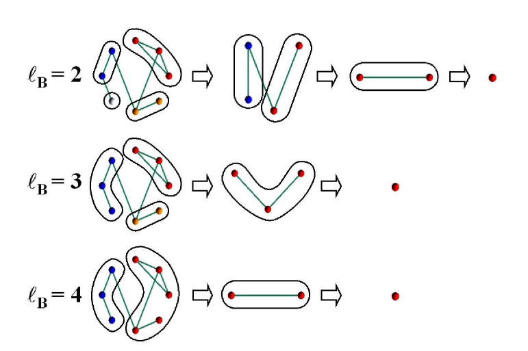
b

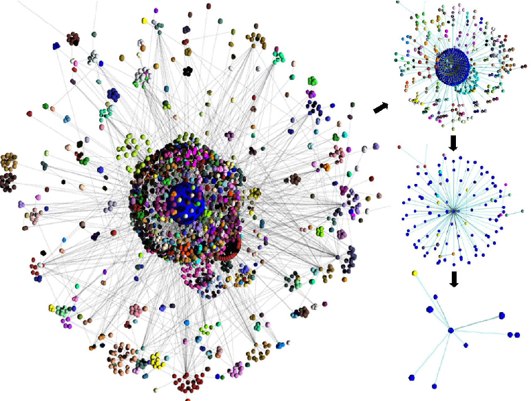
Figure 1:

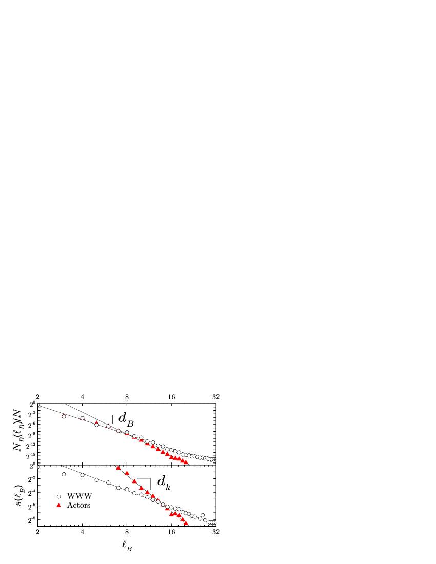
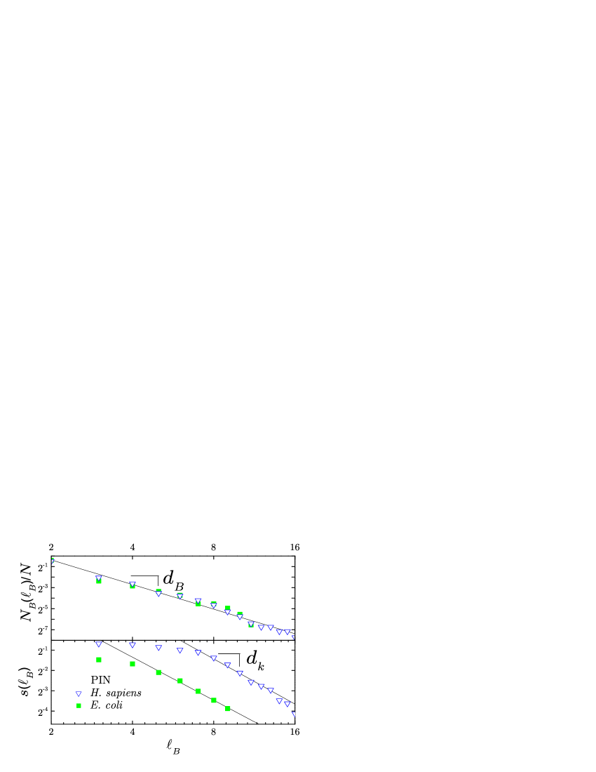
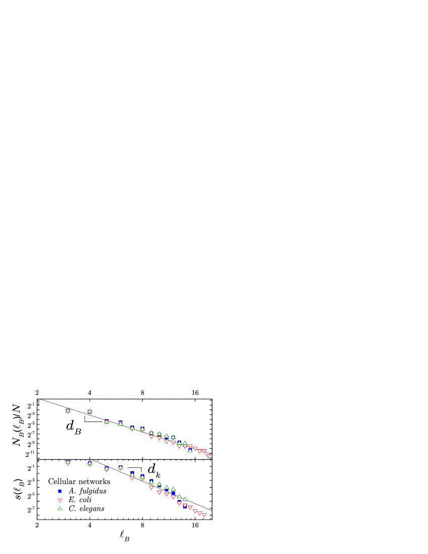
a b c d

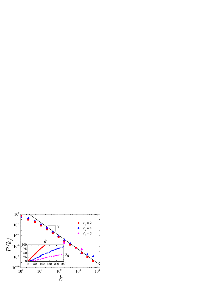
Figure 2:

a

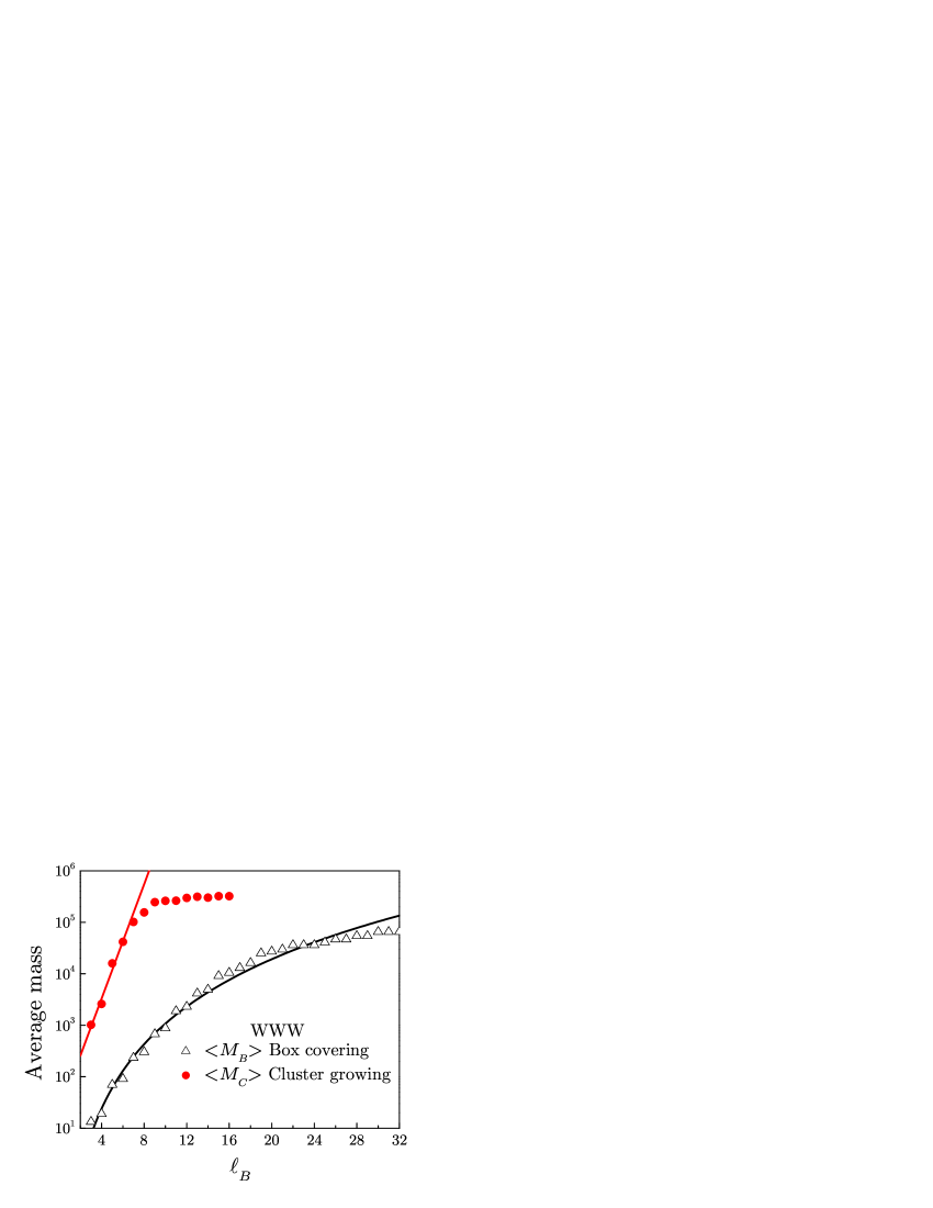
b

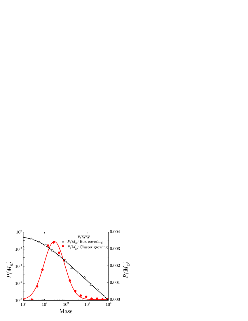
Figure 3:

SUPPLEMENTARY MATERIALS

I The box covering method

Since the box covering method is central to the understanding of the scale-invariant properties of networks, we describe it in more detail here. Figure 4a shows the same network as in Fig. 1a for the case $\ell_{B}=2$. We tile the system by first assigning nodes 1 and 2 to the box colored in blue. Notice that the maximum distance between the nodes of a given box is $\ell_{B}-1$. Thus, node 8 would not be in the blue box since its distance from node 2 is $\ell=2$ (even though its distance from 1 is $\ell=1$). Then we cover the nodes 6 and 7 with the orange box, and the nodes 3, 4, and 5 with the red box. Finally, the last node 8 is assigned to the green box. The number of boxes to cover the network is then $N_{B}=4$.

The renormalization is then applied by replacing each box by a single node. Thus, nodes 1 and 2 will be combined into a single node as indicated by the arrow from the first panel to the second panel in Fig. 4a. This renormalized node is connected with the orange and green boxes because there is a link between nodes 2 and 7, and 1 and 8, respectively. The same rule applies to the other boxes. The renormalized network is shown in the second panel. The system is then tiled again with boxes; in this case two boxes (blue and red) are needed to cover the entire network. The two boxes are then replaced by nodes and a second renormalized network is obtained as shown in the third panel. Finally, the last two nodes belong to the same (red) box and are replaced by a single node.

This procedure is applied to the WWW in Fig. 1b. The main panel corresponds to the first stage in the renormalization of the web for $\ell_{B}=3$. The procedure is applied again obtaining the remaining panels in Fig. 1b until the web is reduced to a single box in the last panel. The colors of the nodes corresponds to the boxes to which they belong.

a

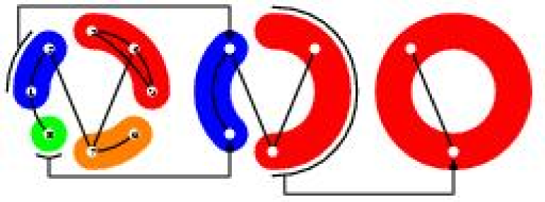
b

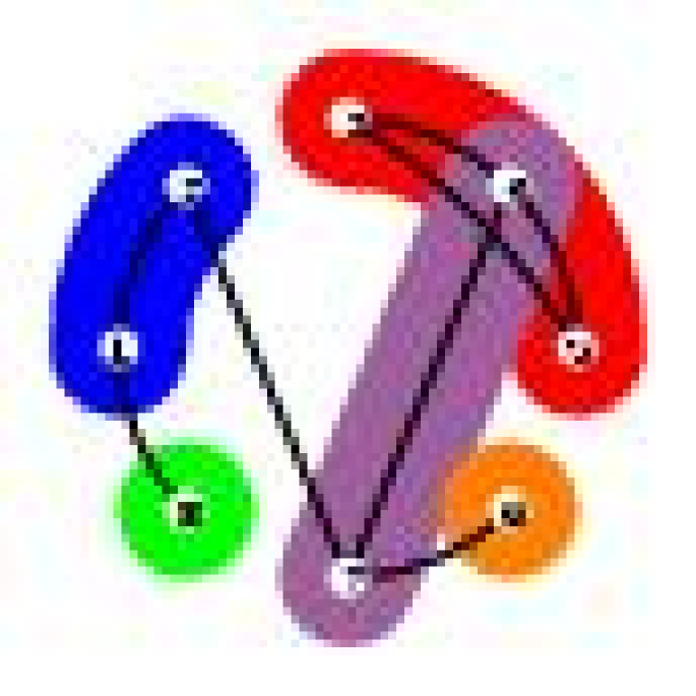
Figure 4: Details of the box covering method for a, $\ell_{B}=2$. b, A different covering for the same network as in (a) for $\ell_{B}=2$. Different coverings give raise to the same exponents as explained in the text.

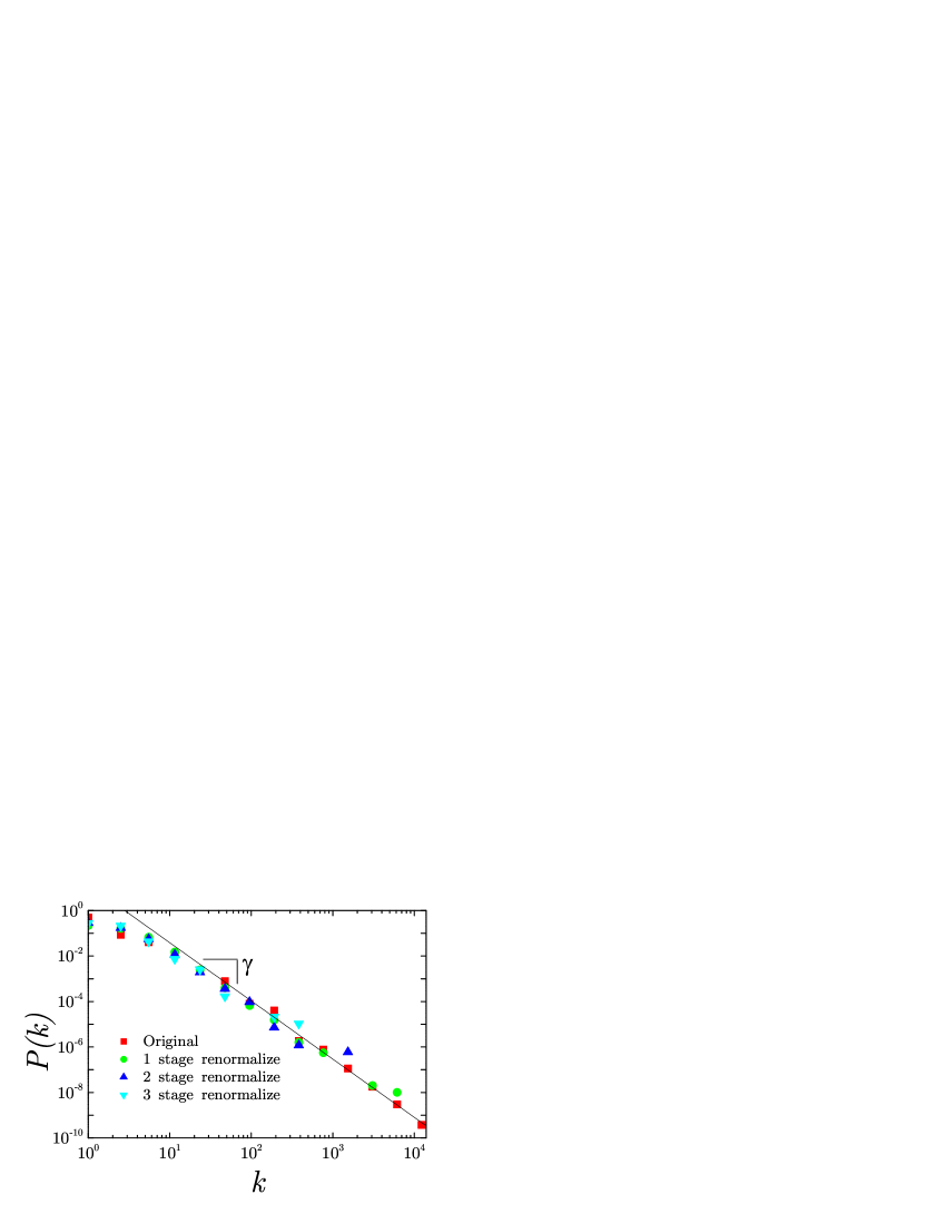
Figure 5: Invariance of the degree distribution of the WWW under multiple renormalizations done at fixed $\ell_{B}=3$. The stages 1, 2, and 3 correspond to the networks depicted in the first three stages in Fig. 1b.

In Fig. 2d we show the invariance of the degree distribution $P(k)$ under the renormalization performed as a function of the box size in the WWW. The other networks analyzed in this study present the same invariant property. It is important to mention that the networks are also invariant under multiple renormalizations applied for a fixed box size $\ell_{B}$. This corresponds, for instance, to the stages depicted in Fig. 1a in the second row for $\ell_{B}=3$ for the network demo. Figure 5 shows the invariance of $P(k)$ for the WWW after several stages of the renormalization for a fixed $\ell_{B}=3$, and it is the analogous of Fig. 2d for different box size. The stages 1, 2, and 3 correspond to the networks depicted in the first 3 stages in Fig. 1b.

From the above explanation it should be clear that there are many ways to tile the network. For instance in Fig. 4b we show another tiling. In this case we assign nodes 4 and 7 together in a single box instead of nodes 6 and 7 as in Fig. 4a. This tiling results in an extra box needed to cover node 6 and therefore in a larger number of nodes to tile the system, $N_{B}=5$.

While there are many ways to assign nodes to the boxes, we notice that the rigorous mathematical definition of Eq. (3) corresponds to the minimum number of boxes needed to cover the network feder . This minimization does not have any consequence for the determination of the fractal dimension in homogeneous clusters. However, it may become relevant when calculating the self-similar exponent of a complex network with a widely distributed number of links. Finding the minimum number of boxes to cover the network is a hard optimization problem to solve, analogous to the graph coloring problem in the NP-complete complexity class. This minimization problem has to be solved by an exhaustive numerical search since there is no numerical algorithm to solve this kind of problems.

We have performed the search over a limited part of the phase-space for the WWW to obtain an estimation of the average and the minimum number of boxes needed to tile the network for every value of $\ell_{B}$. We find that the average value of the boxes is very close to the estimated minimum number of boxes. Moreover, we find that the minimization is not relevant and any covering gives rise to the same exponent.

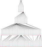
a b

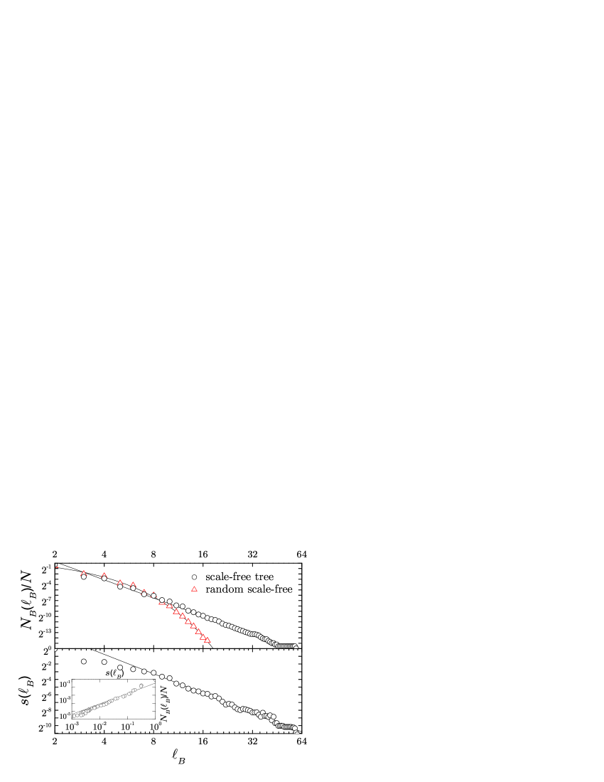
Figure 6: The scale-free tree structure and the random scale-free model. a, Example of a scale-free tree structure. Nodes with a power-law degree distribution are connected in a tree structure without loops. b, The log-log plot of $N_{B}$ vs $\ell_{B}$ reveals a self-similar structure for the scale-free tree (upper panel) while $s(\ell_{B})$ scales as in Eq. (9) (lower panel). In contrast the random scale-free network where nodes (with a power-law distribution of links) are connected at random shows a lack of self-similarity expressed in the exponential decrease with $\ell_{B}$ in the upper panel.

II Scale-free tree structure

The underlying meaning of the existence of scale-free networks which are self-similar is yet to be deciphered, but some insight can be gained by examining the simplest structure of a known network of that kind: a tree network which has been characterized using field theoretical arguments and fractal dimensions in burda .

The sequence of renormalization steps depicted in Fig. 1 suggests the following scheme: one begins with a single node and then constructs the network by applying the renormalization procedure in a reversed fashion. This can be achieved by following the procedure in Fig. 1 for a specific value of $\ell_{B}$.

More specifically, a single node with a large number of links is first connected to the next generation of nodes. For every node we assign a number of links from a power-law distribution with a given $\gamma$. The next layer of the tree is generated in the same way. A tree structure with a power-law degree distribution and self-similar topology emerges which is depicted in Fig. 6a.

This is corroborated numerically in Fig. 6b where we study a scale-free tree structure with 192,827 nodes and $\lambda=2.3$, and we find $d_{B}=3.4$ and $d_{k}=2.5$. The parallels between the features of such a simple structured network and those discussed in this paper suggest that this simplified view may lie at the core of more complex self-similar networks.

Moreover, we also calculate the average mass of the boxes and the mass of the clusters in the box covering method and the cluster covering method, respectively, and we find the power law of Eq. (5) and the exponential behaviour of Eq. (6) (see Fig. 7a) in agreement with the results of the real networks analyzed in the main manuscript, Fig. 3a. Figure 7b shows the probability distribution of $M_{B}$ (power-law) and $M_{c}$ (log-normal) in agreement with previous results as well, Fig. 3b.

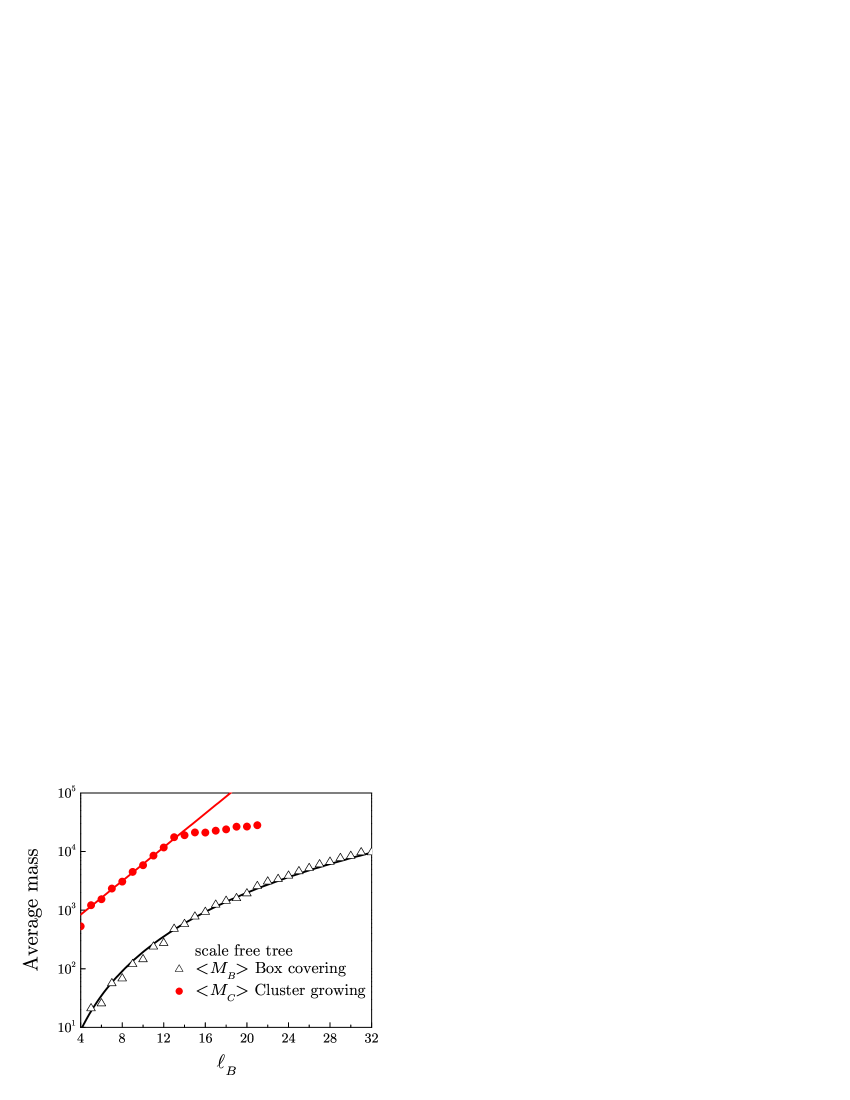
a b

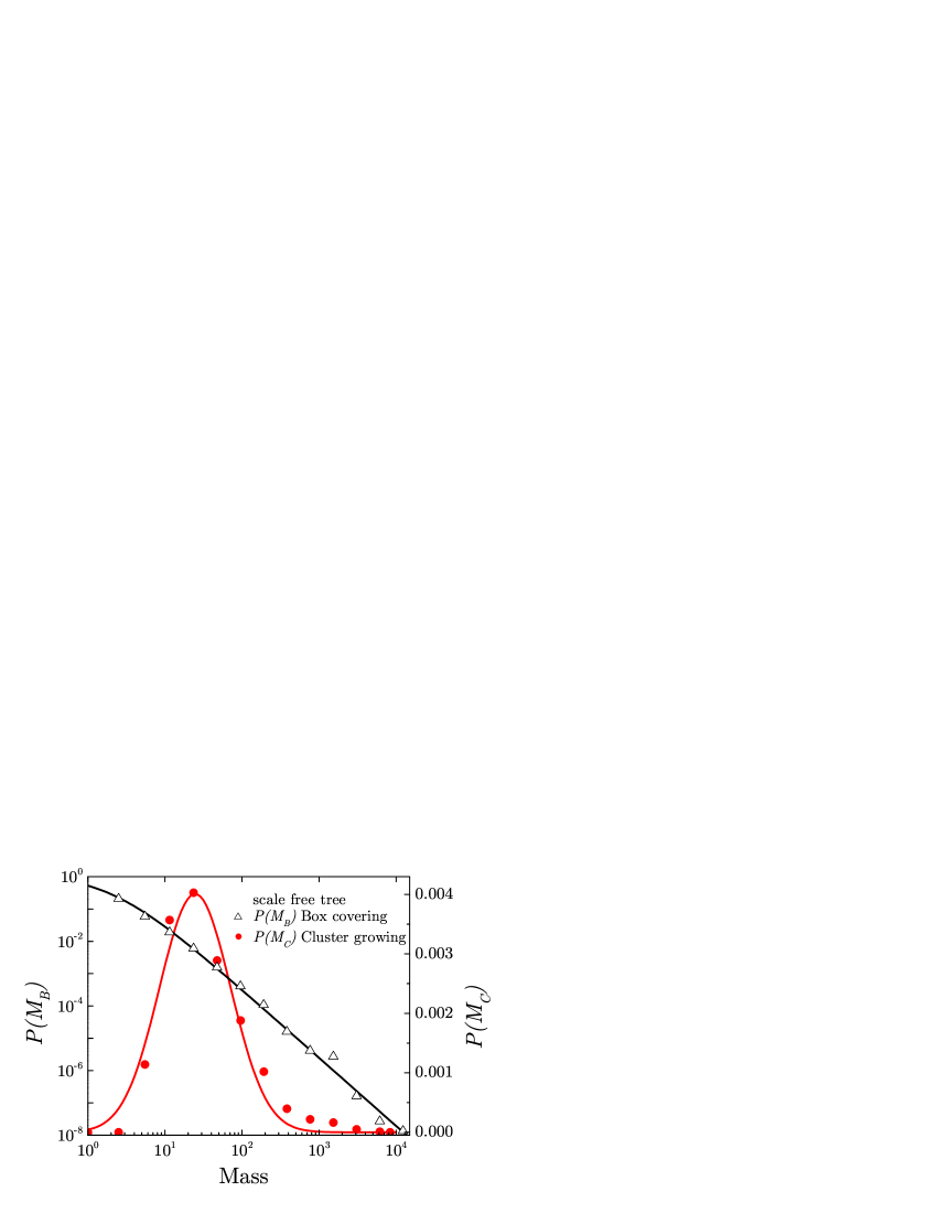
Figure 7: Results for the scale-free tree model. a, Mean value of the box mass in the box counting, $\langle M_{B}\rangle$, and mean value of the cluster mass in the cluster growing method, $\langle M_{c}\rangle$ versus $\ell_{B}$. b, Probability distribution of $M_{B}$ and $M_{c}$ for $\ell_{B}=5$. The results are in agreement with the finding of real networks in Fig. 3. A power-law distribution is found for $M_{B}$ while a log-normal distribution is found for $M_{c}$ as shown by the fits.

III Internet

It is interesting to note that not all complex networks show the clear self-similarity of the networks presented so far. We analyze the Internet composed of computers and routers linked by physical lines such as the database collected by the SCAN project (the “Mbone”, www.isi.edu/scan/scan.html, we also analyze the database of the Internet Mapping Project lucent and found similar results). Figure 8 shows the result of $N_{B}(\ell_{B})$. We fit the curve with a modified power-law

$$N_{B}(\ell_{B})\sim(\ell_{B}+\ell_{c})^{-d_{B}},$$ (11)

with $\ell_{c}=14.9$ representing a cut-off and $d_{B}=8.5$, suggesting a large self-similar exponent. The decay of $N_{B}$ with $\ell_{B}$ is faster than a power-law and slower than exponential as shown in the inset of Fig. 8.

Thus these networks lack the clear self-similar structure found for the WWW, actors and the biological networks. However, we find that the distribution of $P(M_{B})$ remains a power law and the degree distribution $P(k)$ is invariant under the renormalization suggesting that some self-similar properties might still be valid for the Internet. We notice that Internet maps are made by programs that use the IP protocol to trace the connections between each registered node in the Internet. These maps are incomplete since they map a few routers from each domain and also due to the existence of firewalls. Thus, the apparent lack of self-similarity might be due to incomplete information of the network.

IV Protein-protein interaction networks

Figure 8: Internet. Log-log plot of $N_{B}(\ell_{B})$. The solid line represents the modified power law fit, Eq. (11). The inset shows a linear-log plot indicating that the decay is slower than exponential.

We also analyze the protein interaction networks of the fruit fly D. melanogaster as given in dm , the bacterium H. pylori rain , the baker’s yeast S. cerevisiae sc , and the nematode worm C. elegans ce , which are all available via the DIP database dip . Figure 9 shows the results of $N_{B}$ versus $\ell_{B}$ indicating that their behaviour is in between a pure power-law decay and a pure exponential. As with the Internet data, we are able to fit the results with Eq. (11) with $\ell_{c}=7.2$ and $d_{B}=7.6$ for C. elegans. For H. pylori and D. melanogaster the fit is a pure exponential $N_{B}(\ell_{B})\sim\exp(-\ell_{B}/\ell_{e})$ with $\ell_{e}\approx 1$, while for S. cerevisiae the data could be fitted either by an exponential or by large values of $\ell_{c}$ and $d_{B}$ (note that the exponential is the limit of Eq. (11) for $\ell_{c}\to\infty$, $d_{B}\to\infty$ and $\ell_{c}/d_{B}=$ constant). On the other hand, we observe that for small scales, $N_{B}$ seems to display the same power law found for E. coli and H. sapiens. The lack of clear self-similarity in these networks might be due to the incompleteness of these databases which are continuously being updated with newly discovered physical interactions xenarios .

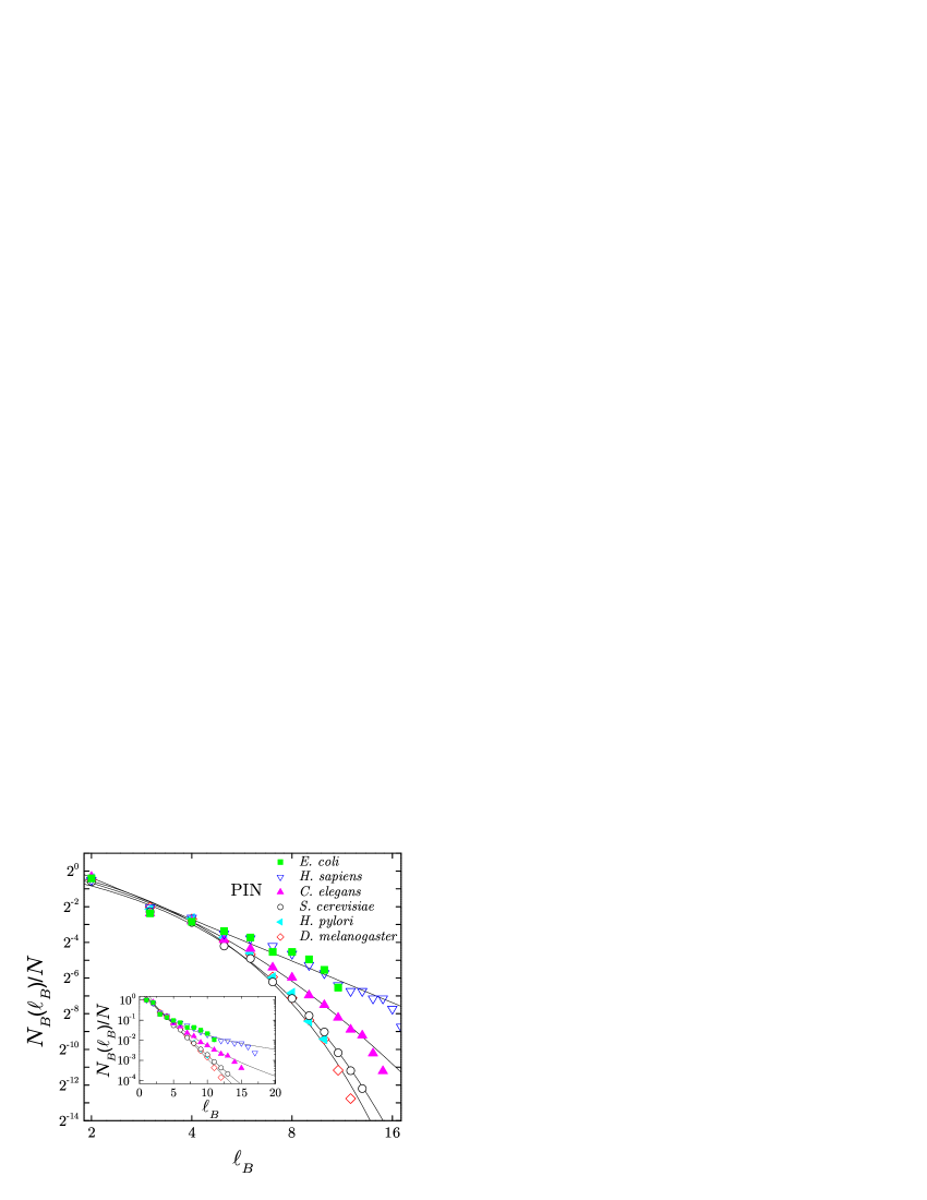
Figure 9: Scaling for the protein-protein interaction networks. Log-log plot of $N_{B}$ versus $\ell_{B}$ for different protein-protein interaction networks. While E. coli and H. sapiens show a clear power law behavior, the other protein networks show a modified power-law behaviour or a pure exponential decay. The inset shows a linear-log plot of $N_{B}(\ell_{B})$.

V Random scale-free network

Next we introduce an example of a model lacking self-similarity: the random scale-free model. This model consists of nodes to which a number of links are assigned with a power-law degree distribution and then connected randomly. Such a network shows a small world effect and a scale-free property but is not self-similar. We numerically find that the number of boxes decays exponentially with the box size (see Fig. 6b). Moreover, while Eq. (8) is still valid in this case, the power law relation in Eq. (9) is replaced by an exponential law. We conjecture that the reason for this is a clustering of hubs; by assigning randomly the connections between the nodes, two nodes with a large number of links will have a large probability to be connected. This induces spatial correlations in the values of $k$ which may explain the breakdown of self-similarity. In contrast, the simple tree-structure proposed above does not cluster the hubs by construction. A summary of our results is presented in Table 1.

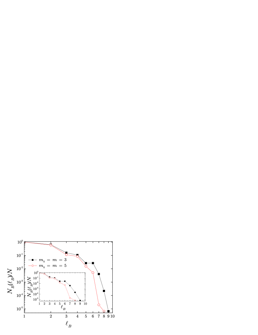
Figure 10: Barabási-Albert model of scale-free networks with preferential attachment for 150,000 nodes and $m=m_{0}=3$ and $m=m_{0}=5$. $m_{0}$ is the initial number of nodes in the system and $m$ is the number of links of a newly created node in the dynamical growth of the network ba . Log-log plot of $N_{B}$ versus $\ell_{B}$ showing the lack of a power law behaviour. The inset shows a linear-log plot indicating that $N_{B}$ decreases faster than exponential with $\ell_{B}$.

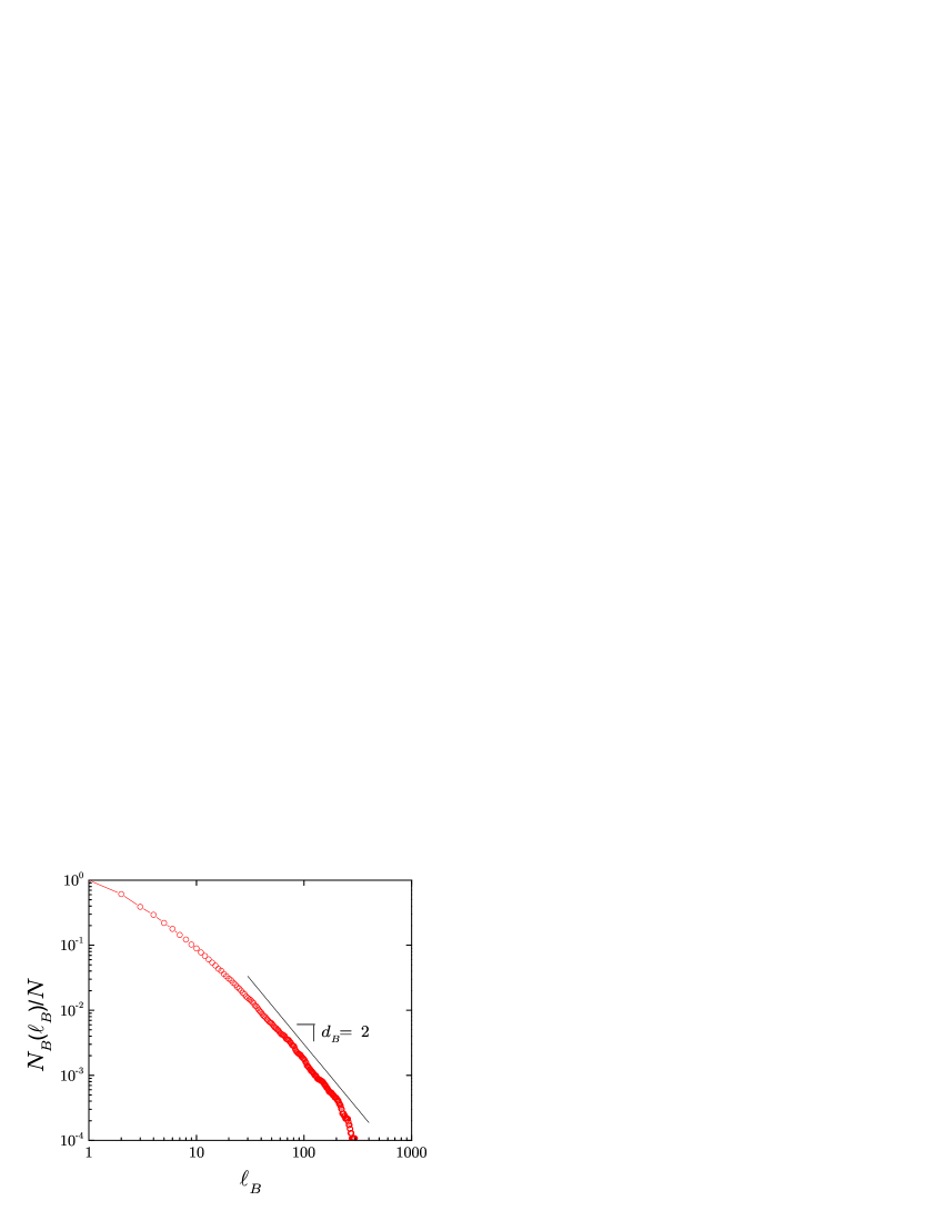
Figure 11: Erdös-Rényi random graph at criticality. Log-log plot of $N_{B}$ versus $\ell_{B}$ showing the self-similar exponent $d_{B}=2$ which is obtained for large distances.

VI The Barabási-Albert model and the Erdös-Rényi random graph at criticality

We also analyzed the Barabási-Albert model of complex networks ba (which introduces the concepts of preferential attachment to describe the dynamics of scale-free networks). The results of $N_{B}(\ell_{B})$ are shown in Fig. 10 for different parameters in the model (see ba for details) reveling that the structure is not self-similar; $N_{B}$ seems to decrease faster than exponential with $\ell_{B}$.

It is interesting to compare our results with the random Erdös-Rényi graph erdos ; bollobas at the critical percolation threshold. In this case the largest cluster has self-similar properties and Eq. (5), $\langle M_{B}(\ell_{B})\rangle\sim\ell_{B}^{d_{B}}$, is valid with $d_{B}=2$ braunstein . We corroborate this result in Fig. 11 showing the scaling of the number of boxes $N_{B}$ with the box size $\ell_{B}$. However, for this case the network is not small-world since Eq. (6) is not valid— as well as Eq. (1)— but rather the mean distance $\bar{\ell}$ scales as $\langle M_{c}\rangle^{1/2}$, i.e., a power-law relation rather than the logarithmic relation characteristic of small world networks.

Network	$d_{B}$	$d_{k}$	$1+d_{B}/d_{k}$	$\gamma$
			Eq. (10)	Eq. (2)
WWW	4.1	2.5	2.6	$2.6$
Actor	6.3	5.3	2.2	$2.2$
E. coli (PIN)	2.3	2.1	2.1	$2.2$
H. sapiens (PIN)	2.3	2.2	2.0	$2.1$
43 cellular networks	3.5	3.2	2.1	$2.2$
Scale-free tree	3.4	2.5	2.4	$2.3$

Table 1: Summary of the exponents obtained for the scale-invariant networks studied in the manuscript.

VII Cellular networks

The WIT database cellular (http://igweb.integratedgenomics.com/IGwit) of cellular networks considers the cellular functions divided according to bioengineering principles containing datasets for intermediate metabolism and bioenergetics (core metabolism), information pathways, electron transport, and transmembrane transport. The metabolic network is a subset of all reactions that take place in the cell. Since this is the largest part of the network we analyze it separately and compare it with the full biochemical reaction network. The data presented in Fig. 2c represents the full biochemical reaction networks of only three substrates. Here we present results of the 43 different substrates represented in the database for the metabolic and full networks. The following figures show the results of $N_{B}$ vs $\ell_{B}$. Both the metabolic and full networks display the power law relationship of self-similar networks with the same exponent (within error bars) for all the organisms considered (the metabolic networks show a finite size effect due to their smaller size). We find an average $d_{B}=3.5$. The solid line in the figures represent the average fit. The values are reported in Table 1.

Aquifex aeolicus

Actinobacillus actinomycetemcomitans

Archaeoglobus fulgidus

Aeropyrum pernix

Arabidopsis thaliana

Borrelia burgdorferi

Bacillus subtilis

Clostridium acetobutylicum

Caenorhabditis elegans

Campylobacter jejuni

Chlorobium tepidum

Chlamydia pneumoniae

Chlamydia trachomatis

Synechocystis sp.

Deinococcus radiodurans

Escherichia coli

Enterococcus faecalis

Emericella nidulans

Haemophilus influenzae

Helicobacter pylori

Mycobacterium bovis

Mycoplasma genitalium

Methanococcus jannaschii

Mycobacterium leprae

Mycoplasma pneumoniae

Mycobacterium tuberculosis

Neisseria gonorrhoeae

Neisseria meningitidis

Oryza sativa

Pseudomonas aeruginosa

Pyrococcus furiosus

Porphyromonas gingivalis

Pyrococcus horikoshii

Streptococcus pneumoniae

Rhodobacter capsulatus

Rickettsia prowazekii

Saccharomyces cerevisiae

Streptococcus pyogenes

Methanobacterium thermoautotrophicum

Thermotoga maritima

Treponema pallidum

Salmonella typhi

Yersinia pestis

References

- (1) Albert R. & Barabási, A.-L. Statistical mechanics of complex networks. Rev. Mod. Phys 74, 47-97 (2002).
- (2) Dorogovtsev, S. N. & Mendes, J. F. F. Evolution of Networks: From Biological Nets to the Internet and the WWW (Oxford University Press, Oxford, 2003).
- (3) Pastor-Satorras, R. & Vespignani, A. Evolution and Structure of the Internet: a Statistical Physics Approach (Cambridge University Press, Cambridge, 2004).
- (4) Newman, M. E. J. The structure and function of complex networks. SIAM Review 45, 167-256 (2003).
- (5) Amaral, L. A. N. & Ottino, J. M. Complex networks - augmenting the framework for the study of complex systems. Eur. Phys. J. B 38, 147-162 (2004).
- (6) Albert, R. Jeong, H. & Barabási, A.-L. Diameter of the World Wide Web. Nature 401, 130-131 (1999).
- (7) Faloutsos, M., Faloutsos, P. & Faloutsos, C. On power-law relationships of the Internet topology. Computer Communications Review 29, 251-262 (1999).
- (8) Erdös, P. & Rényi, A. On the evolution of random graphs. Publ. Math. Inst. Hung. Acad. Sci. 5, 17-61 (1960).
- (9) Bollobás, B. Random Graphs (Academic Press, London, 1985).
- (10) Milgram, S. Psychol. Today 2, 60 (1967).
- (11) Watts, D. J. & Strogatz, S. H. Collective dynamics of ”small-world” networks. Nature 393, 440-442 (1998).
- (12) Bunde, A. & Havlin, S. Fractals and Disordered Systems, edited by A. Bunde and S. Havlin, 2nd edition (Springer-Verlag, Heidelberg, 1996).
- (13) Vicsek, T. Fractal Growth Phenomena, 2nd ed., Part IV (World Scientific, Singapore, 1992).
- (14) Feder, J. Fractals (Plenum Press, New York, 1988).
- (15) Barabási, A.-L. & Albert, R. Emergence of scaling in random networks. Science 286, 509-512 (1999).
- (16) Xenarios, I. et al. DIP: the database of interacting proteins. Nucleic Acids Res. 28, 289-291 (2000).
- (17) Database of Interacting Proteins (DIP). http://dip.doe-mbi.ucla.edu
- (18) Jeong, H, Tombor, B., Albert, R., Oltvai Z. N. & Barabási, A.-L. The large-scale organization of metabolic networks. Nature 407, 651-654 (2000).
- (19) Overbeek, R. et al. WIT: integrated system for high-throughput genome sequence analysis and metabolic reconstruction. Nucleic Acid Res. 28, 123-125 (2000).
- (20) Schopenhauer, A. Transcendent Speculation on the Apparent Deliberateness in the Fate of the Individual, in Parerga and Paralipomena: Short Philosophical Essays, Vol. I, pp. 199-225 (Oxford University Press, Oxford, 1974).
- (21) Burda, Z., Correia, J. D. & Krzywicki, A. Statistical ensemble of scale-free random graphs Phys. Rev. E 64, 046118 (2001).
- (22) Burch, H. & Cheswick, W. Mapping and Visualizing the Internet. IEEE Computer 32, 4 (1999). http://research.lumeta.com/ches/map
- (23) Giot, L. et al. A protein interaction map of Drosophila melanogaster. Science 302, 1727-1736 (2003).
- (24) Rain, J.-C. et al. The protein-protein interaction map of Helicobacter pylori. Nature 409, 211-215 (2001).
- (25) Uetz, P. et al. A comprehensive analysis of protein-protein interactions in Saccharomyces cerevisiae. Nature 403, 623-627 (2000).
- (26) Li, S. et al. A map of the interactome network of the metazoan C. elegans. Science 303, 540-543 (2004).
- (27) Braunstein, L., Buldyrev, S. V., Cohen, R., Havlin, S. & Stanley, H. E. Optimal paths in disordered complex networks. Phys. Rev. Lett. 91, 168701 (2003).