Networks with given two-point correlations: hidden correlations from degree correlations

Abstract

The paper orders certain important issues related to both uncorrelated and correlated networks with hidden variables. In particular, we show that networks being uncorrelated at the hidden level are also lacking in correlations between node degrees. The observation supported by the depoissonization idea allows to extract distribution of hidden variables from a given node degree distribution. It completes the algorithm for generating uncorrelated networks that was suggested by other authors. In this paper we also carefully analyze the interplay between hidden attributes and node degrees. We show how to extract hidden correlations from degree correlations. Our derivations provide mathematical background for the algorithm for generating correlated networks that was proposed by Boguñá and Pastor-Satorras.

I Introduction

Recently, the techniques of equilibrium and non-equilibrium statistical physics were developed to study complex networks 0a ; 0b ; BArev . This paper is devoted to equilibrium correlated networks, with a special attention given to networks with two point correlations newPRL2002 ; newPRE2003a ; dorCM2002 ; bogPRE2003 ; dorCM2003 .

What does it mean that a network is correlated? In simple words one can say that there exist certain relationships between network nodes. For example, when one considers a social network i.e. a group of people with links given by acquaintance ties one may expect that young people are mostly surrounded by other young people. One may also expect that wealthy individuals are more often associated with other wealthy individuals than with poor once. In some sense, the above examples let one suppose that social networks are positively correlated, at least when one considers individual’s age or income. The situation is more contentious if one asks for relationship between gender of the nearest neighbors. Now, it is difficult to assess if social networks are positively or negatively correlated. The above examples show that even taking into account a single network one can observe correlations at different levels of the system complexity. Each node $i$ in such a system has assigned a set of different attributes like: gender $g_{i}$, age $a_{i}$, education $e_{i}$, attractiveness $k_{i}$ etc. The last property may be quantified as a number of nearest neighbors of the considered individual. In the graph theory wilson_book the quantity is known as node’s degree.

The above outlined network correlations and multilevel structure constitute two main issues undertaken in this paper.

Multilevel topology has been recently considered by several groups of researchers gohPRL2001 ; calPRL2002 ; sodPRE2002 ; sodPRE2003a ; sodPRE2003b and, at present, the proposed models are known as random networks with hidden variables. To be precise, to our knowledge, none of the proposed models considers the number of complexity levels larger than two bogPRE2003 i.e. each node $i$ is characterized by at most two parameters: hidden attribute $h_{i}$ and node’s degree $k_{i}$. In general, random networks with hidden variables have a fixed number of vertices $N$. Each node in a network belonging to this class of models has assigned a hidden variable $h_{i}$ (fitness, tag) randomly drawn from a fixed probability distribution $R(h)$ (throughout the paper we use the symbol $R$ with reference to distributions at hidden level and $P$ with reference to node degrees). Edges are assigned to pairs of vertices $\{i,j\}$ with a given connection probability $r_{ij}$. In the simplest case $r_{ij}$ depends only on values of the hidden variables $h_{i}$ and $h_{j}$, but in a more general situation it may for example involve hidden variables characterizing the nearest or the next-nearest neighbors of both considered nodes $i$ and $j$. In fact, the first case represents networks with at most two-point correlations at the level of hidden variables, while the latter one allows for higher order correlations.

Below we outline the concept of network correlations in a more rigorous way. The introduced ideas will be completed and widely discussed in the next section.

From the mathematical point of view, the lack of two point correlations means that the probability $R(h_{j}/h_{i})$, that an edge departing from a vertex $i$ of property $h_{i}$ arrives at a vertex $j$ of property $h_{j}$, is independent of the initial vertex $i$ newPRE2001 ; afCM2005a . The above translates into the fact that the nearest neighborhood of each node is the same (in statistical terms). On the other hand, when $R(h_{j}/h_{i})$ depends on both $h_{i}$ and $h_{j}$ one says that the studied network has two-point correlations newPRE2003a ; bogPRE2003 . To characterize this type of correlations one usually takes advantage of the joint, two-dimensional distribution $R(h_{i},h_{j})$ that describes the probability of randomly chosen edge to connect vertices labeled as $h_{i}$ and $h_{j}$.

In order to characterize network in a more detailed way the concept of higher order correlations, given by multidimensional probability distributions, should be used. In this paper we limit ourselves to two-point correlations. The lack of higher order correlations is ensured by the factorization of the conditional distribution $R(h^{(1)},h^{(2)},\dots,h^{(x)}/h)=R(h^{(1)}/h)R(h^{(2)}/h)\dots R(h^{(x)}/h)$, that describes the probability of a node of property $h$ to have $x$ neighbors labeled as $h^{(1)},h^{(2)},\dots,h^{(x)}$. Such networks, with the only two-point correlations are called Markovian, due to the reason that they are completely defined by the joint distribution $R(h_{i},h_{j})$, which on its own turn completely determines the conditional distribution $R(h_{j}/h_{i})$ and the distribution of hidden variables $R(h)$. Relationships between $R(h_{i},h_{j})$, $R(h_{j}/h_{i})$, $r_{ij}$ and $R(h)$ will be analyzed later.

After this short introduction to the concept of hidden variables and to the problem of network correlations we may go back to the main topic of the paper i.e. the interplay between different levels of the network complexity. The approach has been initiated by Söderberg sodPRE2002 and developed by Boguñá and Pastor-Satorras bogPRE2003 . Boguñá and Pastor-Satorras have concentrated on the question: how correlations at the level of hidden variables affect pattern of connections at the level of node degrees. Given $R(h_{i},h_{j})$ the authors have derived an analytical expression for the joint distribution of degrees of the nearest neighbors $P(k_{i},k_{j})$. In this paper, we ask the reverse question: what kind of hidden correlations $R(h_{i},h_{j})$ produces the given pattern of node degree correlations $P(k_{i},k_{j})$.

As a matter of fact, since most of us are better acquainted with node degree notation than with abstract hidden variables, the reverse approach seems to be very interesting, at least from the methodological point of view. It is already well-known that there exist degree correlations in real networks newPRL2002 . On the other hand, due to the lack of data nothing is known about correlation at the hidden level, from which the observed network structure arises. The paper represents a small step towards understanding the phenomenon of self-organization in complex networks beyond the predominant approach of the so-called evolving networks BAScience ; BAPhysA1999 .

The paper is organized as follows. In Sec. II we review general results on correlated random networks with hidden variables bogPRE2003 . The salient issues concerning two-point correlations are discussed in this section. Sec. III is devoted to theoretical aspects of our reverse problem. Some remarks on uncorrelated networks and a practical algorithm of generating random networks with two-point degree correlations are also given in this section. Finally, in Sec. IV we draw our conclusions.

II Correlated networks with hidden variables

II.1 Construction procedure

Probably the most attractive feature of random networks with hidden variables is the construction procedure that consists of only two steps:

• first, prepare $N$ nodes and assign them hidden variables independently drawn from the probability distribution $R(h)$,

• next, each pair of nodes $\{i,j\}$ link with a probability $r_{ij}$.

Note that the above procedure does not include any ambiguous instructions like in the case of $\dots$ do $\dots$. The lack of ambiguities enables analytical treatment of the discussed models.

The particularly simple model of sparse random networks with hidden variables has been recently considered by Boguñá and Pastor-Satorras. Provided that the connection probability scales according to

$$r_{ij}=\frac{f(h_{i},h_{j})}{N},$$ (1)

where $f(h_{i},h_{j})=f(h_{j},h_{i})$, the authors have shown that the degree distribution of nodes characterized by a fixed value of hidden variable $h$ is given by the Poisson distribution

$$g(k/h)=\frac{e^{-h}h^{k}}{k!}.$$ (2)

The last result is very important because it joins the two levels of the network complexity and allows to freely move between the notation of hidden variables and the notation of node degrees (see section III). In particular, taking advantage of (2), one can see that the average connectivity of nodes characterized by $h$ is simply $h$

$$\langle k\rangle(h)=\sum_{k}kg(k/h)=h,$$ (3)

i.e. hidden variables play the role of desirable degrees. Next, due to (2), the degree distribution $P(k)$ gains a simple form of convolution

$$P(k)=\int R(h)g(k/h)dh.$$ (4)

The last relation between both distributions $P(k)$ and $R(h)$ implies relation between their moments

$$\langle h^{n}\rangle=\langle k(k-1)\dots(k-n+1)\rangle,$$ (5)

and respectively

$$\langle h\rangle=\langle k\rangle,\;\;\;\;\;\;\;\langle h^{2}\rangle=\langle k(k-1)\rangle.$$ (6)

As a matter of fact, in the case of other pair-related distributions, like $R(h_{i},h_{j})$ and $P(k_{i},k_{j})$, it is also possible to obtain relations similar to (4). However, before we proceed with the interplay between hidden variables and node degrees, we would like to discuss the issue of two-point correlations.

II.2 Two-point correlations

One usually thinks about a network as about a collection of nodes and links. Distribution of hidden variables $R(h)$ is the basic characteristic of the set of nodes, whereas the joint distribution $R(h_{i},h_{j})$, describing two-point correlations, applies to the set of edges (see Fig.1). Both distributions express the probability that a random representative of its own ensemble has assigned a given attribute i.e. property $h$ in the case of node and pair of hidden variables $\{h_{i}$, $h_{j}\}$ in the case of edge.

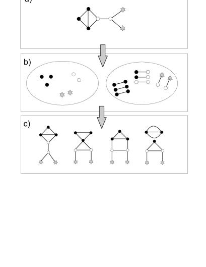
Figure 1: Schematic representation of an ensemble of random networks with a given two-point correlations at the level of hidden variables. Detailed description of the figure is given in the text.

At the moment, let us briefly comment on the Fig.1. The second stage of the figure shows the set of nodes and the set of links, both corresponding to the simple network presented at the first stage of the same figure. Obviously, basing only on the two sets is almost impossible to recreate the original network. Such a representation related to a single network neglects much information. What is lacking are higher order correlations. On the other hand, the joint distribution $R(h_{i},h_{j})$ characterizing the set of edges conveys all the information that is required to construct an ensemble of Markovian random networks (see the third stage of the Fig.1). In fact, all the calculations performed in this paper are related to such an ensemble.

For a given network in the thermodynamic limit, both distributions $R(h)$ and $R(h_{i},h_{j})$ may be defined in the following way

$$R(h)=\frac{N(h)}{N},$$ (7)

and

$$R(h_{i},h_{j})=\frac{E(h_{i},h_{j})}{E},$$ (8)

where $N(h)$ gives the number of nodes assigned by $h$ and $N=\int N(h)dh$, whereas $E(h_{i},h_{j})$ describes the number of links labeled as $\{h_{i},h_{j}\}$ and due to the normalization condition $E=\int\int E(h_{i},h_{j})dh_{i}dh_{j}$.

The connection probability $r_{ij}$ (1) may be simply expressed by the ratio between the actual number of edges connecting vertices of tags $h_{i}$ and $h_{j}$ and the maximum value of this quantity

$$r_{ij}=\frac{E(h_{i},h_{j})}{E_{max}(h_{i},h_{j})}.$$ (9)

Since, during the network construction process one analyzes all pairs of nodes, the maximum number of the considered connections is given by $E_{max}=N(h_{i})N(h_{j})$. Now, taking advantage of (8) the expression for $r_{ij}$ may by rewritten in the following form

$$r_{ij}=\frac{\langle h\rangle R(h_{i},h_{j})}{NR(h_{i})R(h_{j})}.$$ (10)

To fulfill discussion on two point correlations it is necessary to find relation between the two distributions (7) and (8). The relation is encoded in the so-called detailed balance condition

$$R(h_{j}/h_{i})=\frac{\langle h\rangle R(h_{i},h_{j})}{h_{i}R(h_{i})}.$$ (11)

Summing both sides of the last identity over $h_{j}$ ($\int R(h_{j}/h_{i})dh_{j}=1$) one obtains

$$R(h_{i})=\frac{\langle h\rangle}{h_{i}}\int R(h_{i},h_{j})dh_{j}.$$ (12)

As a truth, almost all the above derivations that have been done for hidden variables also hold for node degrees (see bogEPJ2004 ). In particular, the degree detailed balance condition possesses the same form as (11)

$$P(k_{j}/k_{i})=\frac{\langle k\rangle P(k_{i},k_{j})}{k_{i}P(k_{i})}$$ (13)

and respectively the degree distribution in Markovian networks is given by the relation analogous to (12)

$$P(k_{i})=\frac{\langle k\rangle}{k_{i}}\sum_{k_{j}}P(k_{i},k_{j}).$$ (14)

II.3 Interplay between hidden variables and node degrees

Each node of the considered networks is characterized by two parameters: hidden variable $h$ and degree $k$. The probability $p(k\cap h)$ that two given parameters $h$ and $k$ meet together in a certain node is described by the below identity

$$p(k\cap h)=R(h)g(k/h)=P(k)g^{*}(h/k).$$ (15)

The meaning of both conditional distributions $g(k/h)$ and $g^{*}(h/k)$ is simple. The first distribution $g(k/h)$ (2) has just been introduced. It describes the probability that a node labeled by $h$ has $k$ nearest neighbors. The second distribution $g^{*}(h/k)$ is complementary to the first one and gives the probability that a node with $k$ nearest neighbors is labeled by $h$.

The knowledge of $g(k/h)$ and $g^{*}(h/k)$ allows one to find the relation between the joint distributions $R(h_{i},h_{j})$ and $P(k_{i},k_{j})$ characterizing pair correlations respectively at the level of hidden variables and at the level of node degrees. Simple arguments let one describe the interplay by the following relation info

$$P(k_{i},k_{j})=\int\int g(k_{i}-1/h_{i})R(h_{i},h_{j})g(k_{j}-1/h_{j})dh_{i}dh_{j}.$$ (16)

The last expression states that if one knows hidden correlations then it is possible to calculate degree correlations. Relating the problem to the present state of the art in the field of complex networks it is a very artificial situation. The concept of networks with hidden variables is still little-known because most of researchers are strongly attached to the node degree notation. From this point of view, the reverse problem that would answer the question: what kind of hidden correlations produces given degree correlations, seems to be very attractive. In addition, since one knows how to construct Markovian networks with hidden variables, the solution of the above problem would also allow, in a simple way, to generate networks with given two-point degree correlations. We work out the problem in the next section entitled ”Degree correlations from hidden correlations”.

In fact, the idea of generating networks with given degree correlations by means of networks with hidden variables originates from Boguñá and Pastor-Satorras. The authors have argued that since the conditional probability $g(h/k)$ is Poissonian (2), the joint distribution for node degrees (16) approaches the joint distribution for hidden variables for $k_{i},k_{j}\gg 1$

$$P(k_{i},k_{j})\simeq R(k_{i},k_{j}),$$ (17)

and respectively asymptotic behavior of the degree distribution is given by

$$P(k_{i})\simeq R(k_{i}).$$ (18)

The range of convergence of the two distributions has been estimated by Dorogovtsev dorCM2003 , who has shown that both approximations (17) and (18) are only acceptable when $R(h_{i},h_{j})$ and $R(h)$ are sufficiently slowly decreasing.

III Hidden correlations from degree correlations

III.1 Depoissonization

At the moment, let us examine Eq. (4) more carefully. Depending on whether $h$ is discrete or continuous variable the expression for $P(k)$ is respectively discrete or integral transform with Poissonian kernel PT1 . The issue of determining $R(h)$ from $P(k)$ is simply the problem of finding the inverse transform PT2 and one can show that for a given $P(k)$ there exists a unique $R(h)$ which satisfies (4). When $h$ is continuous one gets (see Appendix)

$$R(h)=e^{h}\mathcal{F}^{-1}[G(ix)],$$ (19)

where $\mathcal{F}^{-1}$ denotes the inverse Fourier transform and $G(x)$ describes generating function for the degree distribution $P(k)$

$$G(x)=\sum_{k}x^{k}P(k).$$ (20)

In the case of discrete $h$, the inverse Poisson transform is given by the formula

$$R(h)=e^{h}\mathcal{Z}^{-1}[G(-\ln x)],$$ (21)

where $\mathcal{Z}^{-1}$ describes the inverse Z-transform.

The same applies for the joint degree distributions characterizing two-point correlations. Since

$$g(k-1/h)=\frac{k}{h}\;g(k/h),$$ (22)

the formula (16) may be rewritten as

$$\frac{P(k_{i},k_{j})}{k_{i}k_{j}}=\int\int g(k_{j}/h_{j})\frac{R(h_{i},h_{j})}{h_{i}h_{j}}g(k_{i}/h_{i})dh_{i}dh_{j}.$$ (23)

Now, it is easy to see that $P(k_{i},k_{j})$ is connected with $R(h_{i},h_{j})$ by the two-dimensional Poisson transform and

$$\frac{R(h_{i},h_{j})}{h_{i}h_{j}}=e^{h_{i}+h_{j}}\;\mathcal{F}^{-1}[\mathcal{F}^{-1}[G^{*}(ix,iy)]],$$ (24)

where

$$G^{*}(x,y)=\sum_{k_{i}}\sum_{k_{j}}x^{k_{i}}y^{k_{j}}\frac{P(k_{i},k_{j})}{k_{i}k_{j}}.$$ (25)

The last two expressions can be simply translated for the case of discrete hidden variables. Since however Fourier transforms are more convenient to work with then Z-transforms, we have decided to pass over such a reformulation.

III.2 Some remarks on uncorrelated networks

As we said at the beginning of this paper - the lack of pair correlations at the level of hidden variables means that the conditional probability $R_{o}(h_{j}/h_{i})$ does not depend on $h_{i}$ (to differentiate between uncorrelated and correlated networks the characteristics related to the former case have been denoted by the subscript ’o’). In fact, it is simple to show that

$$R_{o}(h_{j}/h_{i})=\frac{h_{j}}{\langle h\rangle}R_{o}(h_{j}),$$ (26)

and respectively the joint distribution (11) gains a factorized form

$$R_{o}(h_{i},h_{j})=\frac{h_{i}R_{o}(h_{i})h_{j}R_{o}(h_{j})}{\langle h\rangle^{2}}.$$ (27)

Inserting the above expression into (9) one gets the formula for the connection probability in uncorrelated networks

$$r^{o}_{ij}(h_{i},h_{j})=\frac{h_{i}h_{j}}{\langle h\rangle N}.$$ (28)

Now, the question is: does the lack of pair correlations at the hidden level translates to the lack of pair correlations between degrees of the nearest neighbors? Inserting (27) into (16), and then taking advantage of the degree detailed balance condition (13) one gets the answer

$$P_{o}(k_{j}/k_{i})=\frac{k_{j}}{\langle k\rangle}P_{o}(k_{j}),$$ (29)

i.e. the lack of hidden correlations results in the lack of node degree correlations. Thus, in order to generate uncorrelated network with a given degree distribution $P(k)$ one has to:

• prepare the desired number of nodes $N$,

• label each node by a hidden variable randomly taken from the distribution $R(h)$ given by (19) or (21),

• each pair of nodes link with the probability $r^{o}_{ij}$ (28).

(See also other methods for generating random uncorrelated networks with a given degree distribution newPRE2001 ; krzPRE2001 ).

Note also that, due to properties of the Poisson propagator (3)

$$h_{i}=\langle k(h_{i})\rangle\;\;\;\;\mbox{and}\;\;\;\;h_{j}=\langle k(h_{j})\rangle,$$ (30)

therefore the connection probability $r_{ij}^{o}(h_{i},h_{j})$ (28) may be considered as the connection probability $p_{ij}^{o}(k_{i},k_{j})$ between two nodes of degrees $k_{i}$ and $k_{j}$ averaged over all pairs of nodes possessing hidden variables respectively equal to $h_{i}$ and $h_{j}$

$$r^{o}_{ij}(h_{i},h_{j})=\sum_{k_{i}}\sum_{k_{j}}g(k_{i}/h_{i})\;p^{o}_{ij}(k_{i},k_{j})\;g(k_{j}/h_{j}),$$ (31)

where

$$p^{o}_{ij}(k_{i},k_{j})=\frac{k_{i}k_{j}}{\langle k\rangle N}.$$ (32)

The last expression describing connection probability in uncorrelated sparse networks has been already used by several authors (in particular see afPRE2004 ; afCM2002 ; chung2002 ; newPRE2003b ).

III.3 Examples of uncorrelated networks

1. Classical random graphs of Erdös and Rènyi. The degree distribution in ER model is Poissonian

$$P(k)=\frac{e^{-\langle k\rangle}\langle k\rangle^{k}}{k!}\;\;\;\;\;\;\;k\geq 0.$$ (33)

The first step towards calculation of the required distribution $R(h)$ is finding characteristic function for Poisson distribution. Taking advantage of (20) one gets

$$G(x)=e^{\langle k\rangle(x-1)}.$$ (34)

Now, inserting the exponential function into (19) or (21) one can see that the distribution of hidden variables in classical random graphs is respectively given by the Dirac’s delta function (in the case of continuous $h$) or the Kronecker delta (in the case of discrete $h$)

$$R(h)=\delta(h-\langle k\rangle).$$ (35)

The above result means that all vertices are equivalent and the connection probability at the level of hidden variables (28) is given by

$$r^{o}_{ij}=\frac{\langle k\rangle}{N}.$$ (36)

Fig. 2 presents probability $p^{o}_{ij}(k_{i},k_{j})$ of a connection between two nodes characterized by degrees $k_{i}$ and $k_{j}$ in ER model and other uncorrelated networks. As one can see, there exists a very good agreement between the formula (32) and results of numerical calculation.

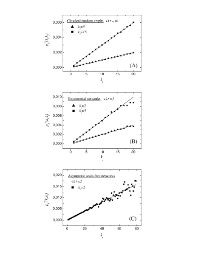
Figure 2: Connection probability $p_{ij}^{o}(k_{i},k_{j})$ in classical random graphs (A), uncorrelated networks with exponential degree distribution (37) (B) and asymptotic scale-free networks (44) (C). Points represent results of numerical calculations averaged over $500$ networks of size $N=5000$.

2. Networks with $P(k)$ given by exponential distribution. Now, let us suppose that

$$P(k)=\frac{\langle k\rangle^{k}}{(1+\langle k\rangle)^{k+1}}\;\;\;\;\;\;\;k\geq 0.$$ (37)

The generating function of the above degree distribution is given by the sum of the geometric series

$$G(x)=\frac{1}{1+\langle k\rangle-\langle k\rangle x}$$ (38)

and (19) provides the exponential distribution of hidden variables (see Fig. 3)

$$R(h)=\frac{e^{-h/\langle k\rangle}}{\langle k\rangle},\;\;\;\;\;\;\;h\geq 0.$$ (39)

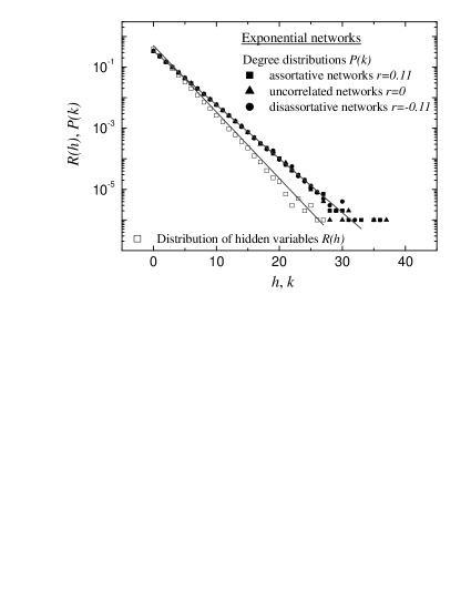
Figure 3: Distribution of hidden variables and degree distributions obtained from numerical simulations of uncorrelated and correlated exponential networks.

3. Scale-free networks. In mathematical terms, the scale-free property translates into a power-law degree distribution

$$P(k)=\frac{A}{k^{\alpha}},\;\;\;\;\;\;\;k\geq 1$$ (40)

where $\alpha$ is a characteristic exponent and $A$ represents normalization constant. Generating function for this distribution is given by the polylogarithm

$$G(x)=A\sum_{k=1}^{\infty}\frac{x^{k}}{k^{\alpha}}=A\;{\mbox{L}}{\mbox{i}}_{\alpha}(x).$$ (41)

To derive distribution of hidden variables that leads to uncorrelated scale-free network one has to find the inverse Fourier transform of the polylogarithm with imaginary argument

$$R(h)=e^{h}\mathcal{F}^{-1}[{\mbox{L}}{\mbox{i}}_{\gamma}(ix)],$$ (42)

or the adequate inverse Z-transform.

Unfortunately, it does not appear that a closed-form solutions for both inverse transforms can be simply obtained. Nevertheless, some asymptotic results for scale-free networks can be derived. In particular, one can show that power law distribution of hidden variables

$$R(h)=\frac{(\alpha-1)m^{(\alpha-1)}}{h^{\alpha}},\;\;\;\;\;\;\;h\geq m,$$ (43)

leads to asymptotic scale-free networks with degree distribution given by

$$P(k)=(\alpha-1)m^{(\alpha-1)}\frac{\Gamma(k-\alpha+1,m)}{k!},$$ (44)

where $\Gamma(x,y)$ is incomplete gamma function. In the limit of large degrees $k\gg 1$ the above degree distribution decays as $P(k)\sim k^{-\alpha}$ (see Fig. 4). The effect of structural cutoffs in power law distributions of hidden variables with $\alpha<3$ (43), imposing the largest hidden variable to scale as $h_{max}\sim\sqrt{N}$ (the relation follows from $r_{ij}^{o}\leq 1$ (28)) bogEPJ2004 ; catPRE2004 ; burdaPRE2003 , does not represent any problem in the studied formalism. The effect of $h_{max}$ in the scale-free $R(h)$ may be considered as an exponential cut-off

$$R(h)=\frac{(\alpha-1)m^{(\alpha-1)}}{h^{\alpha}}\exp\left(-\frac{h}{h_{max}}\right).$$ (45)

Due to properties of the Poisson transform PT1 , the above $R(h)$ results in truncated degree distribution (44)

$$P(k)=\frac{\Gamma(k-\alpha+1,m)}{k!}\frac{(\alpha-1)m^{(\alpha-1)}}{(1/h_{max}+1)^{k-\alpha+1}}.$$ (46)

As expected (see discussion of Eq. (18)), in the limit of large degrees the last formula approaches (45).

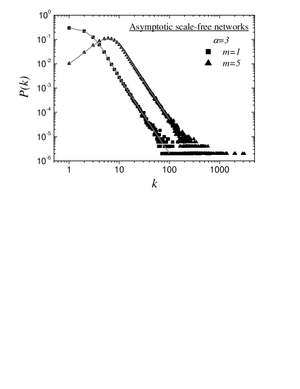
Figure 4: Degree distributions in uncorrelated networks with scale-free distributions of hidden variables (43). Points represent results of numerical calculations whereas solid lines correspond to Eq. (44).

Before we finish with scale-free networks let us, once again, concentrate on the Fig. 4. The figure presents degree distributions $P(k)$ in sparse networks with scale-free distributions of hidden attributes $R(h)$ (43). One can observe that although both distributions converge in the limit of large degrees, there exist serious deviations between (43) and (44) in the limit of small degrees. The relative behavior of the two distributions let one expect that the correct $R(h)$ reproducing the pure scale-free degree distribution $P(k)$ should describe a kind of condensate with a huge number of nodes characterized by a very low values of hidden attributes. On the other hand, despite the ambiguous behavior of $P(k)$ for small degrees, the power-law tail is interesting on his own right. A number of real networks have fat tailed degree distributions. The above allows us to deduce on fat tailed distributions of underlying hidden attributes assigned to individuals co-creating the considered systems.

III.4 How to generate correlated networks with a given degree correlations

Here, we again make use of the depoissonization idea proposed in Sec. III.1. The procedure of generating random networks with a given two-point, degree correlations $P(k_{i},k_{j})$ is as follows:

• first, prepare $N$ nodes,

• next, label each node by a hidden variable randomly taken from the distribution $R(h)$ (19), where $P(k)$ is is given by (14),

• finally, link each pair of nodes with the probability $r_{ij}$ (9), where $R(h_{i},h_{j})$ is calculated according to the formula (24).

Although very clear, the above procedure suffers a certain inconvenience: given a joint degree distribution $P(k_{i},k_{j})$ the closed form solution for $R(h_{i},h_{j})$ (24) is often hard to get. Since however there exists a number of algorithms for numerical inversion of Fourier transform the above does not represent a real problem.

III.5 Examples of correlated networks

To make derivations of previous sections more concrete, we should immediately introduce some examples of correlated networks. In order to simplify the task we will take advantage of general patterns for joint degree distributions with two-point assortative (a) and disassortative (d) correlations that was proposed by Newman newPRE2003a

$$P^{d}(k_{i},k_{j})=\widetilde{P}(k_{i})\widetilde{Q}(k_{j})+\widetilde{Q}(k_{i})\widetilde{P}(k_{j})-\widetilde{Q}(k_{i})\widetilde{Q}(k_{j})\;\;\;$$ (47)

and

$$P^{a}(k_{i},k_{j})=2\widetilde{P}(k_{i})\widetilde{P}(k_{j})-P^{d}(k_{i},k_{j}),$$ (48)

where $\widetilde{P}(k)$ and $\widetilde{Q}(k)$ are arbitrary distributions such that $\sum_{k}\widetilde{P}(k)=\sum_{k}\widetilde{Q}(k)=1$. Assortativity / correlation coefficients newPRL2002 for the above distributions are respectively equal to

$$r^{d}=-\frac{(\mu_{p}-\mu_{q})^{2}}{\sigma_{p}^{2}}\;\;\;\;\;\;\;\;\mbox{and}\;\;\;\;\;\;\;\;r^{a}=-r^{d},$$ (49)

where $\mu_{p}$ represents the expectation value for $\widetilde{P}(k)$, $\mu_{q}$ has the same meaning for $\widetilde{Q}(k)$, whereas $\sigma_{p}^{2}$ corresponds to the variance of $\widetilde{P}(k)$. Now, in order to facilitate further calculations let us assume that

$$\widetilde{P}(k)=\frac{k}{\langle k\rangle}P(k)\;\;\;\;\;\;\mbox{and}\;\;\;\;\;\;\widetilde{Q}(k)=\frac{k}{\langle q\rangle}Q(k),$$ (50)

where

$$\langle k\rangle=\sum_{k}kP(k)\;\;\;\;\;\;\;\mbox{and}\;\;\;\;\;\;\;\langle q\rangle=\sum_{k}kQ(k).$$ (51)

Note that there is no conflict of notation in the last assignment. Putting the two expressions (50) into $P^{a}$ or $P^{d}$ and then taking advantage of the degree detailed balance condition (14) one can easily check that $P(k)$ corresponds to degree distribution. Now, given $P(k)$ one can execute the first two steps (i. and ii.) of the construction procedure described in the previous section.

Inserting the relations (50) into (47) and (48) one obtains (compare it with (23))

$$\frac{P^{d}(k_{i},k_{j})}{k_{i}k_{j}}=\frac{P(k_{i})Q(k_{j})}{\langle k\rangle\langle q\rangle}+\frac{Q(k_{i})P(k_{j})}{\langle k\rangle\langle q\rangle}-\frac{Q(k_{i})Q(k_{j})}{\langle q\rangle^{2}}$$ (52)

and

$$\frac{P^{a}(k_{i},k_{j})}{k_{i}k_{j}}=2\frac{P(k_{i})P(k_{j})}{\langle k\rangle^{2}}-\frac{P^{d}(k_{i},k_{j})}{k_{i}k_{j}}.$$ (53)

Due to linearity of the Poisson transform the joint distributions (52) and (53) turn out to be particularly useful for our purposes. The usefulness means that whenever closed form solutions for the inverse Poisson transforms of $P(k)$ and $Q(k)$ exist, one can also obtain closed form solutions for the joint hidden distributions $R^{d}(h_{i},h_{j})$ and $R^{a}(h_{i},h_{j})$ (24).

Generating functions $G^{*}(x,y)$ (25) for (52) and (53) are respectively given by

$$G^{*}_{d}(x,y)=\frac{G_{p}(x)G_{q}(y)}{\langle k\rangle\langle q\rangle}+\frac{G_{q}(x)G_{p}(y)}{\langle k\rangle\langle q\rangle}-\frac{G_{q}(x)G_{q}(y)}{\langle q\rangle^{2}}$$ (54)

and

$$G^{*}_{a}(x,y)=2\frac{G_{p}(x)G_{p}(y)}{\langle k\rangle^{2}}-G^{*}_{d}(x,y),$$ (55)

where

$$G_{p}(x)=\sum_{k}x^{k}P(k)\;\;\;\;\mbox{and}\;\;\;\;G_{q}(x)=\sum_{k}x^{k}Q(k).$$ (56)

Although visually quite complicated all the above formulas are in fact very simple. Now, in order to perform the last step (iii.) of our procedure aiming at constructing correlated networks, one has to calculate the joint distribution $R(h_{i},h_{j})$. Taking advantage of (24) one gets

$$R^{d}(h_{i},h_{j})=\widetilde{R}(h_{i})\widetilde{S}(h_{j})+\widetilde{S}(h_{i})\widetilde{R}(h_{j})-\widetilde{S}(h_{i})\widetilde{S}(h_{j})$$ (57)

and

$$R^{a}(h_{i},h_{j})=2\widetilde{R}(h_{i})\widetilde{R}(h_{j})-R^{d}(h_{i},h_{j}),$$ (58)

where, similarly to (50) one has

$$\widetilde{R}(h)=\frac{h}{\langle k\rangle}R(h)\;\;\;\mbox{and}\;\;\;R(h)=e^{h}\mathcal{F}^{-1}[G_{p}(ix)],$$ (59)

and also

$$\widetilde{S}(h)=\frac{h}{\langle q\rangle}S(h)\;\;\;\mbox{and}\;\;\;S(h)=e^{h}\mathcal{F}^{-1}[G_{q}(ix)].$$ (60)

Note, that $R(h)$ given in (59) expresses distribution of hidden variables in the considered correlated networks (i.e. the inverse Poisson transform of the degree distribution $P(k)$).

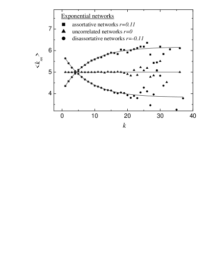
Figure 5: Average nearest neighbor degree $\langle k_{nn}\rangle(k)$ for assortative, uncorrelated and disassortative networks with exponential degree distributions (see section III.5)

Now, let us translate the general considerations into a specific example. Suppose that we are interested in networks with exponential degree distribution (37)

$$P(k)=\frac{\langle k\rangle^{k}}{(1+\langle k\rangle)^{k+1}}\;\;\;\;\;\;\;k\geq 0.$$ (61)

Distribution of hidden variables in such networks is given by (39)

$$R(h)=\frac{e^{-h/\langle k\rangle}}{\langle k\rangle},\;\;\;\;\;\;\;h\geq 0.$$ (62)

For mathematical simplicity, let us assume that the distribution $Q(k)$ responsible for correlations is also exponential

$$Q(k)=\frac{\langle q\rangle^{k}}{(1+\langle q\rangle)^{k+1}}\;\;\;\;\;\;\;k\geq 0.$$ (63)

Given $P(k)$ and $Q(k)$ one has to ensure that the joint hidden distributions (57) and (58) and also the connection probability $r_{ij}$ (9) are positive and smaller than $1$. It is easy to check, that in our case the condition translates into the relation

$$\frac{1}{\sqrt{2}}\leq\frac{\langle q\rangle}{\langle k\rangle}\leq 1.$$ (64)

Now, let us briefly examine the role of $Q(k)$. Depending on the value of $\langle q\rangle$ one obtains stronger or weaker correlations characterized by (49)

$$r^{d}=-\frac{2(\langle k\rangle-\langle q\rangle)^{2}}{\langle k\rangle(\langle k\rangle+1)}\;\;\;\;\;\;\mbox{and}\;\;\;\;\;\;r^{a}=-r^{d}.$$ (65)

In particular, given $\langle k\rangle$ the expression (64) provides possible values for the correlation coefficients that may be reproduced in the considered networks

$$0\leq r\leq\frac{\langle k\rangle}{\langle k\rangle+1}(\sqrt{2}-1)^{2},$$ (66)

where $r=|r^{d}|=|r^{a}|$.

In order to check the validity of our derivations we have performed numerical simulations of correlated networks (47) and (48) with partial distributions given by (61) and (63). Simulations were done for networks ( both assortative and disassortative) of size $N=10^{4}$, $\langle k\rangle=2$ and $\langle q\rangle=\sqrt{2}$. Given $\langle k\rangle=2$, the value of $\langle q\rangle=\sqrt{2}$ corresponds to the maximum value of the correlation coefficient $|r_{max}|=0.11$ (66). At Fig. 3 we depict results corresponding to degree distributions (61) in the considered networks. Fig. 5 presents effects of node degree correlations expressed by the average degree of the nearest neighbor (ANND) that is defined as

$$\langle k_{nn}\rangle(k)=\sum_{k_{i}}k_{i}P(k_{i}/k).$$ (67)

It is already well-known that in the case of uncorrelated networks (29) the ANND does not depend on $k$

$$\langle k_{nn}^{o}\rangle(k)=\frac{\langle k^{2}\rangle}{\langle k\rangle},$$ (68)

whereas in the case of assortatively (disassortatively) correlated systems it is an increasing (decreasing) function of $k$. One can find that in our example the corresponding functions are given by the below formulas

$$\langle k_{nn}^{o}\rangle(k) = 1+2\langle k\rangle,$$ (69)

$$\langle k_{nn}^{d}\rangle(k) = \langle k_{nn}^{o}\rangle(k)-f(k),$$ (70)

$$\langle k_{nn}^{a}\rangle(k) = \langle k_{nn}^{o}\rangle(k)+f(k),$$ (71)

where

$$f(k)=2(\langle k\rangle-\langle q\rangle)\left[1-\left(\frac{\langle q\rangle}{\langle k\rangle}\right)^{k-1}\left(\frac{1+\langle k\rangle}{1+\langle q\rangle}\right)^{k+1}\right].$$ (72)

As one can see (Fig. 5), the fit between computer simulations and the above analytical expressions is very good, certifying the validity of the proposed algorithm (section III.4) for generating random networks with a given degree correlations.

IV Conclusions

In this paper we refer to the set of articles devoted to the so-called random networks with hidden variables. Importance of this paper consists in ordering certain significant issues related to both uncorrelated and correlated networks. In particular, we show that networks being uncorrelated at the hidden level are also lacking in correlations between node degrees. The observation supported by the depoissonization idea (section III.1) allows to extract distribution of hidden variables from a given node degree distribution. Until now the distribution of hidden variables required for generation of a given degree sequence had to be guessed. From this point of view our findings complete the algorithm for generating random uncorrelated networks that was suggested by other authors sodPRE2002 ; chung2002 . We also show that the connection probability in sparse uncorrelated networks is factorized function of node degrees (32).

In this paper we also carefully analyze the interplay between hidden attributes and node degrees. We show how to extract hidden correlations from degree correlations and how to freely move between the two levels of the networks complexity. Our derivations provide mathematical background for the algorithm for generating correlated networks that was proposed by Boguñá and Pastor-Satorras bogPRE2003 .

V Acknowledgments

The authors thank Prof. Janusz A. Hołyst for useful discussions and comments. A.F. acknowledges financial support from the Foundation for Polish Science (FNP 2005) and the State Committee for Scientific Research in Poland (Grant No. 1P03B04727). The work of P.F. has been supported by European Commission Project CREEN FP6-2003-NEST-Path-012864.

VI Appendix

The inverse Poisson transform for the case of continuous $h$ (19) has been derived by E. Wolf and C.L. Mehta in 1964 PT2 . Below we outline the derivation, and then adopt it for the case of discrete $h$ (21).

Our aim it to inverse the formula

$$P(k)=\int_{0}^{\infty}\frac{e^{-h}h^{k}}{k!}R(h)dh.$$ (73)

Let

$$F(x) = \int_{0}^{\infty}e^{ixh}R(h)e^{-h}dh$$

$$= \int_{0}^{\infty}\sum_{k=0}^{\infty}\frac{(ixh)^{k}}{k!}R(h)e^{-h}dh$$

$$= \sum_{k=0}^{\infty}(ix)^{k}P(k)=G(ix),$$

where $G$ (20) represents generating function for the degree distribution $P(k)$. Then by the Fourier inversion formula one gets the expression (19)

$$R(h)=e^{-h}\mathcal{F}^{-1}[G(ix)].$$ (75)

The above derivation can be simply adopted for the case of discrete transform with Poissonian kernel i.e.

$$P(k)=\sum_{h=0}^{\infty}\frac{e^{-h}h^{k}}{k!}R(h).$$ (76)

Let us introduce an auxiliary sequence

$$J(h)=e^{-h}R(h).$$ (77)

It is easy to show that the Z-transform of this sequence equals to generating function of the degree distribution (20)

$$\mathcal{Z}[J(h)] = \sum_{h=0}^{\infty}\frac{J(h)}{s^{h}}$$ (78)

$$= \sum_{h=0}^{\infty}\left(\sum_{l=0}^{\infty}\frac{(-h\ln s)^{l}}{l!}\right)J(h)$$ (79)

$$= \sum_{l=0}^{\infty}(\ln s^{-1})^{l}P(l)=G(\ln s^{-1}).$$ (80)

Applying the inverse Z-transform to the last expression one obtains the formula (21) describing distribution of hidden variables

$$R(h)=e^{h}\mathcal{Z}^{-1}[G(\ln s^{-1})].$$ (81)

References

- (1) S.Bornholdt and H.G.Schuster, Handbook of Graphs and networks, Wiley-Vch (2002).
- (2) S.N. Dorogovtsev and J.F.F.Mendes, Evolution of Networks, Oxford Univ.Press (2003).
- (3) R.Albert and A.L.Barabási, Rev. Mod. Phys. 74 47 (2002).
- (4) M.E.J. Newman, Phys. Rev. Lett. 89, 208701 (2002).
- (5) M.E.J. Newman, Phys. Rev. E 67, 026126 (2003).
- (6) S.N. Dorogovtsev, J.F.F. Mendes and A.N. Samukhin, cond-mat/0206131 (2002).
- (7) M. Boguñá and R. Pastor-Satorras, Phys. Rev. E 68, 036112 (2003).
- (8) S.N. Dorogovtsev, cond-mat/0308336 (2003).
- (9) R.J.Wilson, Intr. to Graph Theory, Longman (1985).
- (10) K.-I. Goh, B. Kahng and D. Kim, Phys. Rev. Lett. 87, 278701 (2001).
- (11) G. Caldarelli, A. Capocci, P. DeLosRios and M.A. Munoz, Phys. Rev. Lett. 89, 258702 (2002).
- (12) B. Söderberg, Phys. Rev. E 66, 066121 (2002).
- (13) B. Söderberg, Phys. Rev. E 68, 015102(R) (2003).
- (14) B. Söderberg, Phys. Rev. E 68, 026107 (2003).
- (15) M.E.J. Newman, S.H. Strogatz and D.J. Watts, Phys. Rev. E 64, 026118 (2001).
- (16) A. Fronczak, P. Fronczak and J.A. Hołyst, cond-mat/0502663 (2005).
- (17) A.L.Barabási and R.Albert, Science 286, 509 (1999).
- (18) A.L.Barabási, R. Albert and H. Jeong, Physica A 272, 173 (1999).
- (19) M. Boguñá, R. Pastor-Satorras and A. Vespignani, Eur. Phys. J. B 38, 205 (2004).
- (20) The formula (16) directly follows from the Eq.(25) given in bogPRE2003 .
- (21) H.J. Hindin, Theory and applications of the Poisson transform, Conference record of second Asilomar conference on circuits and systems. Institute of Electrical and Electronics Engineers Inc. 1968, pp.525-9. New York, NY, USA.
- (22) E. Wolf and C.L. Mehta, Phys. Rev. Lett. 13, 705 (1964).
- (23) Z. Burda, J.D. Correia and A.Krzywicki, Phys. Rev. E 64, 046118 (2001).
- (24) M. Catanzaro, M. Boguna and R. Pastor-Satorras, Phys. Rev. E 71, 027103 (2005).
- (25) A. Fronczak, P. Fronczak and J.A. Hołyst, Phys. Rev. E 70, 056110 (2004).
- (26) A. Fronczak, P. Fronczak and J.A. Hołyst, cond-mat/0212230
- (27) F. Chung and L. Lu, Annals of Combinatorics 6, 125 (2002).
- (28) J. Park and M.E.J. Newman, Phys. Rev. E 68, 026112 (2003).
- (29) Z. Burda and A. Krzywicki, Phys. Rev. E 67, 046118 (2003).