Bond Distortions in Armchair Type Single Wall Carbon Nanotubes

Abstract.

The energy band gap structure and stability of (3,3) and (10,10) nanotubes have been comparatively investigated in the frameworks of the traditional form of the Su-Schrieffer-Heeger (SSH) model and a toy model including the contributions of bonds of different types to the SSH Hamiltonian differently. Both models give the same energy band gap structure but bond length distortions in different characters for the nanotubes.

1. Introduction

A single-wall carbon nanotube (SWCNT) is an empty tube of graphene consisting of hexagonally arranged carbon atoms. In graphene, there are two different rim shapes, armchair and zigzag. For an armchair SWCNT, the hexagon rows are parallel to the tube axis. The $\pi$-electronic structure of an armchair SWCNT arises from the $\pi$-structure of graphene. Each carbon atom in graphene contributes to the structure with one electron in the $2p_{\mathrm{z}}$ orbital perpendicular to the plane of the sheet. Generally, the overlap of $\pi$-orbitals due to the curvature in nanotubes are neglected for moderate curvatures. If $n$ is the number of two-carbon sites (dimers), i.e. the nearest neighbors on polyacetylene (PA) chain which is the prototype polymer of graphene, the nanotube is labeled as ($n$,$n$). One of the most important properties of armchair nanotubes is that they show metallic behavior [1].

In the present treatise the tight-binding approximation, which is sometimes known as the method of linear combination of atomic orbitals, is used. This approximation deals with the case in which the overlap of atomic wave functions is enough to require corrections to the picture of isolated atoms but not so much as to render the atomic description completely irrelevant. It is mostly used for describing the energy bands arising from the partially filled d-shells of transition metal atoms and for describing the electronic structure of insulators. Moreover, the tight-binding approximation provides an instructive way of viewing Bloch levels complementary to that of the nearly free electron picture, permitting a reconciliation between the apparently contradictory features of localized atomic levels on the one hand and free electron-like plane-wave levels on the other [2].

The tight-binding approximation was originally developed by Su-Schrieffer-Heeger (SSH) [3] for conducting polymers (1D systems) and then extended to two-dimensional systems by Harigaya [4, 5]. Harigaya’s model preserves the fixed-length constraint of one-dimensional polymer chain and hence it contains a single Lagrange multiplier. In most applications of this model to graphene and to tubes constructed from graphene, the constraint has still been used in the same form, that is all bond distortions are summed without considering the type of bonds and this sum is assumed to vanish. However, two different types of bonds appear in graphene and so in tubes, tilt and right (see Fig. 1). It would also be worthwhile to point out that bond length difference of hexagon structure have been reported by the calculations on graphene and nanotubes [5, 6].

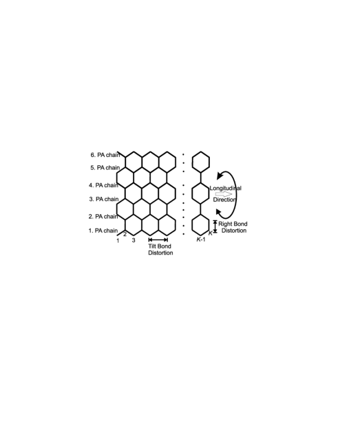
Figure 1. Inter-chain coupling structure of a (3,3) armchair type nanotube and bond distortions.

Considering this fact, in this work on armchair type nanotubes, we present for the first time the modification in Harigaya’s model by taking the contributions of bonds of different types to the SSH Hamiltonian differently. This automatically leads us to separate the constraint into two constraints, vanishing of the sum of right bond distortions and vanishing of the sum of tilt bond distortions. In this way we build a toy model which provides more freedom for lattice relaxations. We have already mentioned the very preliminary results of this toy model in our work in [7]. In our second work [8], we evaluated the electronic band structure of (3,0) nanotube with periodic boundaries in the framework of this toy model and in the Harigaya’s model comparatively. We observed that the tiny energy gap appearing in Harigaya’s model was lost when our toy model has been used. This result consists with the fact that zigzag nanotubes ($n$,0) are metallic when $n$ is any multiple of 3, and semiconducting when $n$ cannot be divided by 3. This is determined by whether the $K$ and $K^{\prime}$ points of the graphite meet with the one-dimensional Brilloune zones determined by the geometry or not.

The ($n$,$n$) armchair nanotubes are always metallic for all the integers $n$ and metallic behavior of (3, 3) armchair nanotube has also experimentally being shown [9, 10]. Recently, Li et al. [11] have grown free-standing SWCNTs. Their diameter is as small as 0.4 nm. The (3,3) armchair nanotubes are among the possible structures of this size [11]. This is why we deal with here with (3,3) armchair nanotube in the framework of our toy model. On the other hand, the commonly observed diameter of SWCNT by experiments is known as about 1.4 nm which corresponds to that of (10,10) SWCNT. Therefore, we also test our toy model with this larger diameter nanotube.

2. MODEL

The SSH model Hamiltonian

(1) $$H_{\mathrm{SSH}}=-\sum_{\langle i,j\rangle,\sigma}\Big{[}t_{0}-\alpha(u_{i}^{(j)}-u_{j}^{(i)})\Big{]}(c^{\dagger}_{i,\sigma}c_{j,\sigma}+\mathrm{h.c.})$$

$$+\frac{\kappa}{2}\sum_{\langle i,j\rangle}\Big{[}(u_{i}^{(j)}-u_{j}^{(i)}-C)^{2}-(C)^{2}\Big{]}\,,$$

which had originally been written for 1D systems, was directly applied to 2D systems without any modification by Harigaya [5]. Here, $\langle i,j\rangle$ is the nearest-neighbor carbon-carbon atom pairs and $t_{0}$ is the hopping integral of the undimerized system. The second term represents the dimerization due to $\sigma$ skeleton with free involving $\pi$-electrons. $\alpha$ is the electron-lattice coupling constant, $\kappa$ is the effective spring constant. The operator $c_{i,\sigma}^{\dagger}$ ($c_{i,\sigma}$) creates (annihilates) a $\pi$-electron at the $i$-th carbon atom with spin $\sigma$. $u_{i}^{(j)}$ is the displacement of the $i$-th atom along the $j$-th one, whereas in the original SSH model Hamiltonian $u_{i}^{(j)}$ is perpendicular to carbon-hydrogen bond direction for both trans-PA and cis-PA. The term $u_{i}^{(j)}-u_{j}^{(i)}$, when considered for trans-PA or cis-PA, denotes the projection of the bond length difference along chain axis. But for nanographite, the same term denotes directly the bond length difference. $C$, in the last term, is the Lagrange multiplier in the self-consistent method which has been inserted in the original SSH Hamiltonian due to the fixed length constraint when it was firstly used for trans-PA and cis-PA [12]. Harigaya preserved the same constraint for 2D systems [4, 5]. This constraint binds the distortions in both the length and circumference directions of the tube and, in a sense, relatively restricts the lattice relaxation.

In trans-PA and cis-PA, all the bonds are of the same type. An armchair (and also a zigzag) SWCNT can be thought of to be built by parallel trans-PA with inter-chain coupling as seen in Fig. 1. Therefore in nanotubes there are two different types of bonds, tilt and right bonds.

During the lattice relaxation, of course, the relative distances between the carbon atoms in hexagons and the angles in hexagons become different. In the toy model, which we wish to built in the present work, as a first approximation we are going to neglect the changes in the angles in hexagons and keep only the changes in the relative distances. Furthermore, we would like to modify the SSH model Hamiltonian by taking the contributions of the two different bond types and rewrite the SSH model Hamiltonian as follows:

$$H_{\mathrm{SSH}} = -\sum_{{\langle i,j\rangle_{\mathrm{t}},\sigma}}\Big{[}t_{0}^{\mathrm{t}}-\alpha^{\mathrm{t}}(u_{i}^{(j)}-u_{j}^{(i)})\Big{]}(c^{\dagger}_{i,\sigma}c_{j,\sigma}+\mathrm{h.c.})$$

$$-\sum_{{\langle i,j\rangle_{\mathrm{r}},\sigma}}\Big{[}t_{0}^{\mathrm{r}}-\alpha^{\mathrm{r}}(u_{i}^{(j)}-u_{j}^{(i)})\Big{]}(c^{\dagger}_{i,\sigma}c_{j,\sigma}+\mathrm{h.c.})$$

$$+\frac{\kappa^{\mathrm{t}}}{2}\sum_{\langle i,j\rangle_{\mathrm{t}}}\Big{[}(u_{i}^{(j)}-u_{j}^{(i)}-C^{\mathrm{t}})^{2}-(C^{\mathrm{t}})^{2}\Big{]}$$

$$+\frac{\kappa^{\mathrm{r}}}{2}\sum_{\langle i,j\rangle_{\mathrm{r}}}\Big{[}(u_{i}^{(j)}-u_{j}^{(i)}-C^{\mathrm{r}})^{2}-(C^{\mathrm{r}})^{2}\Big{]}\,,$$

where $\langle i,j\rangle_{\mathrm{t}}$ and $\langle i,j\rangle_{\mathrm{r}}$ denote tilt and right bonds, respectively. With this separation it seemed to us natural to use two different Lagrange multipliers, $C^{\mathrm{t}}$ and $C^{\mathrm{r}}$. To be able to insert these multipliers in the Hamiltonian we have to consider two constraints: vanishing separately the sum of all tilt bond distortions and the sum of all right bond distortions, i.e. $\sum v_{i,j}^{\mathrm{t}}=0$ and $\sum v_{i,j}^{\mathrm{r}}=0$, where $v_{i,j}\equiv\alpha(u_{i}^{(j)}-u_{j}^{(i)})$. This means that lattice relaxations may gain more freedom. The mean value of the sum in the first constraint is obviously proportional to the length of tube and the mean value of the sum in the second constraint is related to the circumference of tube. As a matter of fact, in the literature Ono and Hamano considered also two constraints during the study of Peierls distortions in a two-dimensional electron-lattice system described by SSH type model [13].

In this case the total energy of the system reads as

(3) $$E_{\mathrm{T}}=\sum_{i,\sigma}^{\prime}\varepsilon_{i,\sigma}+\frac{1}{2\gamma^{\mathrm{t}}}\,\sum_{i}[v_{i}^{\mathrm{t}}]^{2}+\frac{1}{2\gamma^{\mathrm{r}}}\,\sum_{i}[v_{i}^{\mathrm{r}}]^{2}\,,$$

where $\varepsilon_{i,\sigma}$ are the eigenvalues of Eq. (2). The self-consistent equation for the lattice is

(4) $$v_{i}^{{\mathrm{t,r}}}=2\gamma^{{\mathrm{t,r}}}\Big{[}\frac{\alpha^{{\mathrm{t,r}}}C^{{\mathrm{t,r}}}}{\gamma^{{\mathrm{t,r}}}}-\frac{1}{N_{b}^{{\mathrm{t,r}}}}\frac{\gamma^{{\mathrm{t,r}}}}{\alpha^{{\mathrm{t,r}}}}\sum_{j,\sigma}^{\prime}B^{{\dagger}}_{i+1,j,\sigma}B_{i,j,\sigma}\Big{]}\,.$$

where ${\mathbf{B}}$’s are the eigenvectors of Eq. (2) and $\gamma^{\mathrm{t,r}}=(\alpha^{\mathrm{t,r}})^{2}/\kappa^{\mathrm{t,r}}$. The prime means that the sum is over the filled states, the number of which are equal to half of the total number of carbon sites. $N_{\mathrm{b}}^{{\mathrm{t,r}}}$’s are the total number of tilt and right $\pi$-bonds, respectively. Eqs. (2)-(4) are solved numerically by iteration method [7, 8].

3. RESULTS AND DISCUSSIONS

We describe the geometry of nanotubes with bonds. During the numerical evaluations we considered the diameter and lengths of (3,3) tubes as 0.5 nm and 0.73-36.36 nm, respectively since experimentally, 0.4 nm-sized carbon nanotubes have been reported to exist [9-11] and also 0.33 nm-sized carbon nanotubes were also grown from a larger SWCNT inside an electron microscope [14]. For the purpose of checking our numerical evaluations, we have calculated the diameters of (3,3) and (5,0) nanotubes. Although we could find the given diameter for (5,0) nanotube we could not find the given diameters 0.4 nm and 0.33 nm for (3,3) nanotube, instead we found 0.5 nm, when both calculations had been done with the same parameters derived from the experimental work [11]. Moreover, we repeat our numerical calculations for (10,10) nanotube which has the diameter 1.4 nm, the commonly observed diameter of SWCNT by experiments, when the tube length varies between 0.73 nm and 16.0 nm.

The calculations on (3,3) armchair type nanotube is considered with $N=2n$ and the PA chain length $K$ varying between 6 (0.73 nm) and 300 (36.36 nm), that is with maximum 1800 C-atoms. For the (3,3) armchair type open ended nanotube, the number of right bonds is 900 and the number of tilt bonds is 1794 for $K=300$. In the periodic boundaries case, the number of right bonds keeps itself while the number of tilt bonds increases 6 more.

The calculations on (10,10) armchair type nanotube is considered with $N=2n$ and $K$ varying between 6 (0.73 nm) and 132 (16.0 nm), that is with maximum 2640 C-atoms. For the (10,10) armchair type open ended nanotube, the number of right bonds is 1320 and the number of tilt bonds is 2620 for $K=132$. In the periodic boundaries case, the number of right bonds keeps itself while the number of tilt bonds increases 20 more.

Firstly, we studied the electronic band structure as (3,3) armchair nanotube evolves from carbon sheet, in the cases the tube is open ended and possesses periodic boundaries, in the framework of our toy model and in that of Harigaya’s model comparatively by taking $t_{0}$ and $\alpha$ values the same for tilt and right bonds. We realized this by multiplying each one of the hopping integrals responsible for sheet, open ended tube and tube with periodic boundaries by parameters denoted by $\beta_{\mathrm{S}}$, $\beta_{\mathrm{N}}$ and $\beta_{\mathrm{T}}$, respectively and by varying these parameters from zero to one; that is by introducing gradually the interactions characterizing the aforementioned structures. In this way we can show continuously the evolution of electronic band structure as geometry transforms. In both models, we obtained identical electronic band gap structures shown in Fig. 2. Hence, contrary to (3,0) zigzag nanotube [8], there is not any difference between the electronic band structures of metallic (3,3) armchair nanotube regarding both models. We can explain this fact in the following way: The electronic band structure in the scale of the total $\pi$-electron energy bands seem similar, because the bond alternation amplitude is one order of magnitude smaller than that of PA (see Figs. 3. and 4) and the magnitude of $u$ is about 0.03 Å  in trans-PA [3]. The electronic band structure of (10,10) nanotubes gives no significant change in comparison with the electronic band structure given in Fig. 2 for (3,3). Thus we are not going to plot it separately.

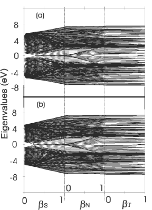
Figure 2. Electronic band structure evolutions from carbon sheet to SWCNT for (3,3) armchair type nanotube with $K=42$ for models including (a) one constraint and (b) two constraints. $\beta_{\mathrm{S}}$, $\beta_{\mathrm{N}}$ and $\beta_{\mathrm{T}}$ represent the evolution parameters for carbon sheet, open ended nanotube and nanotube with periodic boundaries. No band gap appears as expected. For (10,10) nanotube the same electronic band structure was obtained. Only, the marked regions appeared darker. This is because of the jump of the number of energy eigen-values from 504 to 840 when (10,10) nanotube is considered instead of (3,3) for the same $K$ value, $K=42$.

Secondly, we consider the stability problem of (3,3) and (10,10) armchair nanotubes in the framework of both models when nanotubes possess periodic boundaries.

According to the Harigaya’s model, we numerically calculated the bond distortions via the simplified form of Eq. (4). For (3,3) nanotube the results can be expressed as follows (Fig. 3): The right bond distortions are twice of the tilt bond distortions. The right bond distortions are always negative, that is these bonds shrink while the tilt bond distortions are always positive, that is tilt bonds stretch. Besides, at the beginning the distortions increase up to $K=12$ and then tend to decrease. For $K=16$ shrinking of right bonds suddenly turns to stretching and, at the same time, stretching of tilt bonds suddenly turns to shrinking. For $K=22$ there is no bond distortions for both types of bonds. Therefore, the first thing to be noted is that in order to be able to obtain reasonable results in agreement with the literature one must consider the tubes longer than 2.67 nm ($K=22$)[6]. After this special $K$ value (for tubes longer than 2.67 nm), the tube length-oscillations of tilt bond distortions show decaying. The half period of oscillations about some mean tilt bond distortion values is 3. These mean values at first decay and then remain almost the same after $K=212$. This means that, as the length of tube becomes longer, the tilt bond stretching values repeat a decaying increasing-decreasing behavior about almost constant bond distortions. Furthermore, the amplitude of oscillation decays, that is for longer tubes oscillation of tilt bond distortions vanish and after a certain large $K$ value (approximately 400) the bond distortions approach a definite nonzero value. Meanwhile, the right bond shrinkages behave similarly and they also tend to nonzero values. These are unexpected results because it is known that long enough tubes are stable.

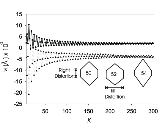
Figure 3. The filled circles and the filled triangles represent the tilt and right bond distortions, respectively when Harigaya’s model is used. $K$ is the number of sites in trans-PA chains. In the inset the forms of hexagons for $K=50,52$ and $54$ are depicted. Since the right bonds always shrink (the amount of shrinkage is maximum for $K=54$ and minimum for $K=52$) and the tilt bonds always stretch (the amount of stretching is minimum for $K=52$ and maximum for $K=54$), the diameter of the tube decreases while it’s length increases.

As for (10,10) nanotube, a repetition of the above evaluations now gives the result summarized in Fig.4(a). There is not any systematic change in the tilt and right bond distortions as $K$ increases. Both of them decay immediately to zero. Hence the tube is stable except for very small $K$ values. This is quite the expected result because wide enough tubes might be stable for smaller $K$ values that correspond to shorter tubes. Therefore the shorter tubes would be necessary in order to observe bond alternations otherwise the longer tubes will show relatively small alternations.

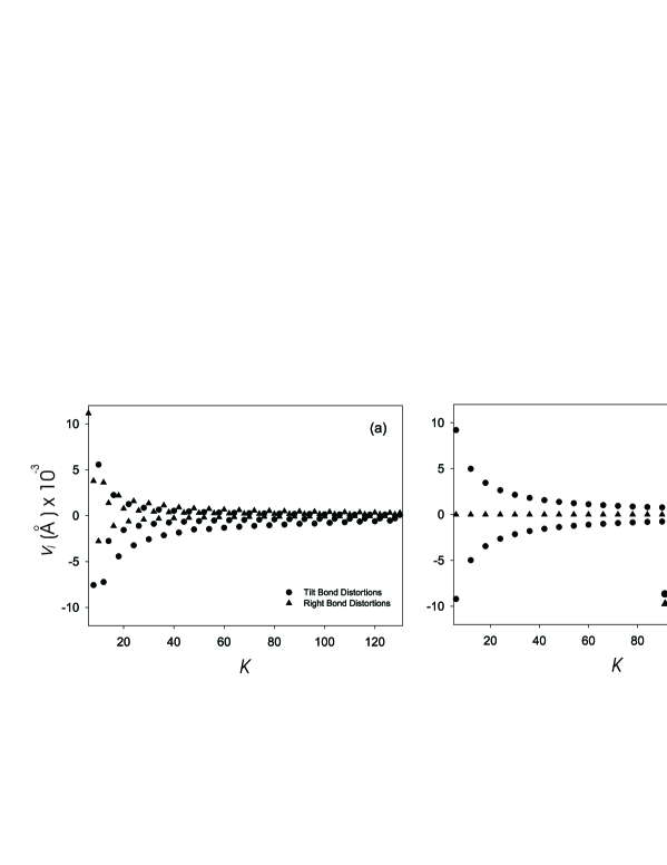
Figure 4. (a) The filled circles and the filled triangles denote the tilt and right bond distortions, respectively when Harigaya’s model is used, for (10,10) nanotube. (b) The bond alternations in the case the toy model is used.

According to our toy model, we consider Eq. (4) for the bond distortions by taking again $t_{0}$ and $\alpha$ values the same for tilt and right bonds. For both (3,3) and (10,10) nanotubes, all the right bond distortions vanish while tilt bond distortions appear as bond alternations when $K$ is divisible by 3. For both (3,3) and (10,10) tubes, the tilt bond distortions vanish also when $K$ is not divisible by 3. Of course, vanishing of tilt bond distortions for $K$ values not divisible by 3 is a handicap for the toy model.

The bond distortions for (3,3) armchair type SWCNT with periodic boundaries are illustrated in Fig. 4. As seen from this figure, equal amount of stretching and shrinkage of alternate bonds occur. The tilt bond alternations start with $\pm 0.0306$ Å  for $K=6$ and drastically fall to $\pm 0.0066$ Å  at $K=36$. In other words, the lattice structure relaxation starts at $K=36$. It is clear that tilt bond alternation values decrease exponentially for small $K$ values while they decrease monotonically for large $K$ values. Although we did the calculations up to $K=400$, we terminated the graphic at $K=300$ since we observed the continuation of monotonic decreasing of tilt bond alternations. At this point, we believe that the explanation of the aforementioned difference in the bond distortions for various $K$ values (multiple of 3 or not) is vital.

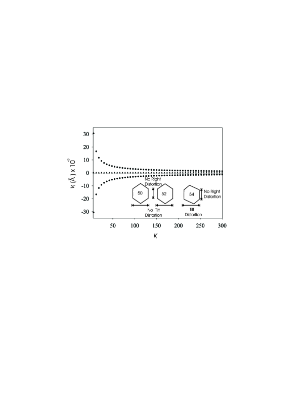
Figure 5. The filled circles and the filled triangles denote the tilt and right bond alternations, respectively when our toy model is used, for $K$ divisible by 3. In the inset the forms of hexagons for $K=50,\,52$ and $54$ are depicted. Neither the diameter nor the length of tube changes.

The bond distortions for (10,10) armchair type SWCNT with periodic boundaries are illustrated in Fig. 4(b). We have the same bond distortion behavior, bond alternations.

To see the strength of dimerization, we plot in Fig.6 the $1/K$ variation of tilt and right bonds and also the average of the absolute values of bond alternations for both (3,3) and (10,10) nanotubes when $K$ is divisible by 3. $\langle|v_{i}|\rangle$ decreases linearly for both tubes. The extrapolated value at $K\to\infty$ is 0.0005 nm [5,15] for (3,3) nanotube (Fig.6(c)). For (10,10) nanotube, $\langle|v_{i}|\rangle$ reaches to zero for $K\approx 10^{4}$ (Fig.6(d)). Moreover, from the $1/K$ variation of the tilt and right bonds one sees the length differences between the long and short bonds to be 0.002 nm and 0 nm, respectively for the (3,3) and (10,10) nanotubes (Fig.6 (a) and (b)).

To bring to a conclusion, although for (3,3) armchair type SWCNTs with periodic boundaries the two models give different stability properties, (10,10) SWCNTs are stable according to both models. But still there is a difference. The toy model puts forth bond alternations. When the size of the bond alternations of (3,3) and (10,10) SWCNTs are compared, a decrease is observed. For instance, for $K=6$ the tilt bond alternations is $\pm 0.0306$ Å for (3,3) and $\pm 0.0009$ Å for (10,10) and for $K=132$ the tilt bond alternations is $\pm 0.0024$ Å for (3,3) and $\pm 0.0005$ Å for (10,10). Hence, the bond alternations diminishes at $66\%$ for $K=132$. Therefore, the tube diameter strongly affects the bond alternation amplitudes.

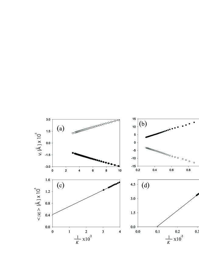
Figure 6. The $1/K$ variation of bond variables. $\langle|v_{i}|\rangle$’s for the (3,3) and (10,10) nanotubes are shown in (a) and (c), respectively- whereas. (b) and (d) show the $v_{i}^{\mathrm{r},t}$.

4. CONCLUSION

In the progress of taking the coefficients of the contributions of the tilt and right bond distortions to the SSH model Hamiltonian differently and following Stafstrom et el.’s work on the inclusion of Lagrange multiplier in the Hamiltonian [12], we have to use two constraints, one for the vanishing of the sum of right bond distortions and the other for the vanishing of the sum of tilt bond distortions. Here, a toy model obtained in this way is applied to calculate the energy band gap and bond variations with the number of rows, $K$, of (3,3) and (10,10) armchair type nanotubes of diameters 0.5 nm and 1.4 nm, respectively. There is not any change in the energy band gap structure in the large energy scale. However contrary to this, bond length alternations, which were absent in the one constraint Harigaya’s model, have been observed when $K$ is divisible by 3. These alternations tend to vanish as the $K$ values increase, that is for long enough tubes. Unfortunately, the vanishing of bond length distortions when $K$ is not divisible by 3 would be an artifact of the model. The non vanishing of the bond distortions even for long enough tubes according to the Harigaya’s model seems to be in contradiction with experimental results for (3,3) nanotubes. For (10,10) nanotubes both models work free of problems.

References

(1) Dresselhaus, M. S., Dresselhaus, G. and Eklund, P. C. In: "Science of Fullerenes and Carbon Nanotubes", New York: Academic Press, 1996, p. 809.

(2) Ashcroft, N. W. and Mermin, N. D., "Solid State Physics", CBS Publishing, Philadelphia, 1988.

(3) Su, W. P., Schrieffer, J. R. and Heeger, A. J., Phys. Rev. B 22 (1980) 2099.

(4) Harigaya, K., J. Phys. Soc. Jpn. 60 (1991) 4001.

(5) Harigaya, K., Phys. Rev. B 45 (1992) 12071.

(6) Cabria, I., Mintmire, J. W. and White, C. T., Int. J. Quant. Chem. 91 (2003) 51.

(7) Sünel, N. and Özsoy, O., Int. J. Quant. Chem. 100 (2004) 231.

(8) Özsoy, O. and Sünel, N., Czech J. Phys., 54 (2004) 1495.

(9) Qin, L. C., Zhao Xi, L., Hirahara, K., Miyamoto, Y., Ando, Y. and Iijima, S., Nature 2000;408(6808):50.

(10) Sun, L. F., Xie, S. S., Liu, W., Zhou, W. Y., Liu, Z. Q., Tang, D. S., Wang, G. and Qian, L. X., Nature 2000;403(6768):384.

(11) Li, G. D., Tang, Z. K., Wang, N. and Chen, J. S., Carbon 40 (2002) 917.

(12) Stafström, S., Riklund, R. and Chao, K. A., Phys. Rev. B 26 (1982) 4691.

(13) Ono, Y. and Hamano, T., J. Phys. Soc. Jpn., 69 (2000) 1769.

(14) Peng, L. M., Zhang, Z. L., Xue, Z. Q., Wu, Q. D., Gu, Z. N. and Pettifor, D. G., Phys. Rev. Lett., 15 (2000) 3249.

(15) Harigaya, K. and Fujita, M., Phys. Rev. B 47 (1993) 16563.