Noise in Disordered Systems: Higher Order Spectra in Avalanche Models

Abstract

Utilizing the Haar transform, we study the higher order spectral properties of mean field avalanche models, whose avalanche dynamics are described by Poisson statistics at a critical point or critical depinning transition. The Haar transform allows us to obtain a time series of noise powers, $H(f_{1},t)$, that gives improved time resolution over the Fourier transform. Using $H(f_{1},t)$ we analytically calculate the Haar power spectrum, the real $1.5$ spectra, the second spectra, and the real cross second spectra in mean field avalanche models. We verify our theoretical results with the numerical results from a simulation of the $T=0$ mean field nonequilibrium random field Ising model (RFIM). We also extend our higher order spectra calculation to data obtained from a numerical simulation of the $T=0$ infinite range RFIM for $d=3$, and experimental data obtained from an amorphous alloy, $Fe_{21}Co_{64}B_{15}$. We compare the results and obtain novel exponents.

I Introduction

There are disordered systems that respond to slow driving with discrete jumps or avalanches with a broad range of sizes, referred to as crackling Nature . Such crackling systems are characterized by many interacting degrees of freedom and strong interactions that make thermal effects negligible, such as: charge density waves, vortices in type II superconductors, crack propagation, earthquakes, and Barkhausen noise in magnets. The avalanche dynamics of the systems mentioned above are described by Poisson statistics (given by Eq. (1)) in mean field theory at a critical point or critical depinning transition Matt1 ; Fisher .

Through our analysis of mean field avalanche models we determine the following spectral functions: Haar power spectrum, real $1.5$ spectra, second spectra, and real cross second spectra for systems that have avalanche dynamics given by Eq. (1). This analysis provides new tools for noise analysis in dynamical systems, since there are very few theoretical calculations of higher order noise statistics.

The Haar transform allows us to obtain a power versus time series, $H(f_{1},t)$, needed to calculate higher order spectra. These higher order spectra give valuable information about the avalanche dynamics in Barkhausen noise not accessible through ordinary power spectra OBrien ; Petta . Higher order spectra also have been used to obtain crucial information about a variety of diverse systems such as: metastable states in vortex flow Merithew , natural auditory signals Thomson , conductance-noise in amorphous semiconductors Parsam , fluctuating current paths in devices Seidler , and quasi-equilibrium dynamics of spin glasses Weissman . While much experimental work has been done studying higher order spectra OBrien ; Petta ; Merithew ; Thomson ; Parsam ; Seidler ; Weissman , we present a rigorous mean field treatment that is applicable to a broad range of systems Fisher . This analysis will allow a better understanding of the dynamics of these systems, and provide a direct method of comparison to experiment or observation.

In addition, we compare our general results from mean field theory to Barkhausen noise obtained: from a mean field simulation of the $T=0$ random field Ising model (RFIM) Dahmen , from a simulation of the $T=0$ infinite range RFIM (IRM) in $d=3$, and from experiment. We also find novel exponents from our analysis, and we compare our results from theory, simulation, and experiment; we find key similarities and differences.

II THE MODEL

II.1 Mean Field RFIM

The $T=0$ mean field RFIM consists of an array of $N$ spins ($s_{i}=\pm 1$), which may point up ($s_{i}=+1$) or down ($s_{i}=-1$). Spins are coupled to all other spins (through a ferromagnetic exchange interaction $J$), and to an external field $H(t)$ which is increased adiabatically slowly. To model disorder in the material, we assign a random field, $h_{i}$, to each spin, chosen from a distribution $P(h_{i})=exp(-h^{2}_{i}/2R^{2})/\sqrt{2\pi}R$, where $R$ determines the width of the Gaussian probability distribution and therefore gives a measure of the amount of quenched disorder for the system. The Hamiltonian for the system at a time $t$ is given by: $H=-\sum\limits_{i}(JM+H(t)+h_{i})s_{i}$, where $M=\frac{1}{N}\sum\limits_{j}s_{j}$ is the magnetization of the system. Initially, $H(-\infty)=-\infty$ and all the spins are pointing down. Each spin is always aligned with its local effective field $h_{i}^{eff}=JM+H(t)+h_{i}$.

II.2 RFIM with infinite range Forces (IRM) in 3D

The $T=0$ Infinite Range RFIM (IRM) consists of a 3D lattice of $N$ spins, with a Hamiltonian at a time $t$ given by: $H=\sum\limits_{<ij>}-Js_{i}s_{j}-\sum_{i}(H(t)+h_{i}-J_{inf}M)s_{i}$, where $J_{inf}>0$ is the strength of the infinite range demagnetizing field, and $\langle ij\rangle$ stands for nearest neighbor pairs of spins. The local effective field is given by $h_{i}^{eff}=J\sum_{<ij>}s_{j}+H(t)+h_{i}-J_{inf}M$.

The addition of a weak $J_{inf}\sim\frac{1}{N}$ to the traditional RFIM causes the system to exhibit self-organized criticality (SOC) Urbach ; Narayan ; Zapperi . This means that as $H$ is increased the model always operates at the critical depinning point, and no parameters need to be tuned to exhibit critical scaling behavior (except $\frac{dH}{dt}\rightarrow 0$). We limit our analysis to a window of $H$ values where the slope of $M(H)$ is constant and the system displays front propagation behavior. Details of the simulation algorithm are given elsewhere Matt2 .

II.3 Avalanche Dynamics in the $T=0$ RFIM

The external field $H(t)$ is adiabatically slowly increased from $-\infty$ until the local field, $h_{i}^{eff}$, of any spin $s_{i}$ changes sign, causing the spin to flip Matt1 ; Sethna . It takes some microscopic time $\Delta t$ for a spin to flip. The spin flip changes the local field of the coupled spins and may cause them to flip as well, etc. This avalanche process continues until no more spin flips are triggered. Each step of the avalanche, that is each $\Delta t$, in which a set of spins simultaneously flip, is called a shell. The number of spins that flip in a shell is directly proportional to the voltage $V(t)$ during the interval $\Delta t$ that an experimentalist would measure in a pick-up coil wound around the sample. In our simulations we denote the number of spins flipped in a shell at a time $t$ by $n_{t}(=V(t))$. The first shell of an avalanche (one spin flip) is triggered by the external field $H(t)$, while each subsequent shell within the avalanche is triggered only by the previous shell, since $H(t)$ is kept constant while the avalanche is propagating. $H(t)$ is only increased when the current avalanche has stopped, and is increased only until the next avalanche is triggered (i.e. $\frac{dH}{dt}\rightarrow 0$). The number of shells in an avalanche times $\Delta t$ defines the pulse duration, $T$, or the time it took for the entire avalanche to flip. The time series of $n_{t}$ values for many successive avalanches creates a Barkhausen train analogous to experiment.

III EXPERIMENT

We compare our results for theory and simulation with results obtained from an experiment performed on an (unstressed) amorphous alloy, $Fe_{21}Co_{64}B_{15}$. Measurements were performed on a 21 cm x 1 cm x 30 $\mu$m ribbon of $Fe_{21}Co_{64}B_{15}$ alloy, a soft amorphous ferromagnet obtained from Gianfranco Durin. The domain walls run parallel to the long axis of the material, with about 50 domains across the width. A solenoid, driven with a triangle wave, applies a magnetic field along the long axis of the sample. Since domain wall motion dominates over other means of magnetization in the linear region of the loop, data were collected in only a selected range of applied fields near the center of the loop. The Barkhausen noise was measured by a small pick-up coil wound around the center of the sample. This voltage signal was amplified, anti-alias filtered and digitized, with care taken to avoid pick-up from ambient fields. Barkhausen noise was collected for both increasing and decreasing fields for $80$ cycles of the applied field through a saturation hysteresis loop. The driving frequency was $0.01$ Hz; this corresponds to $c=0.09$, where c is a dimensionless parameter proportional to the applied field rate and is defined in the Alessandro Beatrice Bertotti Montorsi model (ABBM model) for the Barkhausen effect in metals ABBM . In this way, our measurements should be well inside the $c<1$ regime identified in the ABBM model, in which we can expect to find more or less separable avalanches rather than continuous domain wall motion.

IV THEORY

IV.1 Poisson Distribution

The probability distribution for the avalanche dynamics in the class of mean field avalanche models we are interested in is given by Fisher ; Matt1 :

$$P(n_{0}=1,n_{1},n_{2},...,n_{\infty})=\frac{1}{en_{1}!}\prod\limits^{\infty}_{t=2}\frac{e^{-n_{t-1}}n^{n_{t}}_{t-1}}{n_{t}!}$$ (1)

The above probability distribution (Eq. 1) is for the time series of a single infinite avalanche at the critical point. In the context of the mean field RFIM, $n_{t}$ represents the number of spins flipped at a time $t$. That is, each $n_{t}$ represents a shell of the avalanche, and since an avalanche begins with one spin flip we have that $n_{0}=1$.

Let $\langle.\rangle$ represent the average over Eq. 1. In order to calculate the Haar transform and higher order spectra in mean field theory we need the following quantities, where $m\geq l\geq k\geq 0$ and $j\geq 0$:

$$\langle n_{j}\rangle=1$$ (2)

$$\langle n_{j}^{2}\rangle=j+1$$ (3)

$$\langle n_{j}n_{j+k}\rangle=\langle n_{j}^{2}\rangle=j+1$$ (4)

$$\langle n_{j}^{3}\rangle=\frac{1}{2}(3j^{3}+5j+2)$$ (5)

$$\langle n_{j}^{4}\rangle=\frac{1}{2}(6j^{3}+13j^{2}+9j+2)$$ (6)

$$\langle n_{j}n_{j+k}n_{j+l}\rangle=\langle n_{j}^{3}\rangle+k\langle n_{j}^{2}\rangle$$ (7)

$$\langle n_{j}n_{j+k}n_{j+l}n_{j+m}\rangle$$

$$=\langle n_{j}^{4}\rangle+(2k+l)\langle n_{j}^{3}\rangle+\frac{k}{2}(k+2l-1)\langle n_{j}^{2}\rangle$$ (8)

These relations can be determined from Eq. (1). We notice that the time ordering of the indices plays on important role. Details of how Eqs. (2-IV.1) were derived are given in Appendix A.

IV.2 Haar Power

The Haar transform is a simple wavelet transform with basis states consisting of single-cycle square waves. We use the Haar transform rather than the Fourier transform since it gives us improved time resolution in exchange for less frequency resolution. Time resolution is important to our purpose since we are interested in studying how the power contribution around a frequency $f_{1}$ changes along the duration of the avalanche.

Physically, the Haar power, $H(t,f_{1})$, is the absolute square of the time integral over a period (of duration $1/f_{1}$) of a single-cycle square wave times a section of the train centered around $t$ OBrien . In other words, to determine the Haar power we integrate a square wave of duration $1/f_{1}$ over a section of the noise train centered at time $t$; this integrated segment is then squared to assure our resulting values is positive definite, this squared segment corresponds to $H(t,f_{1})$, the Haar power at time $t$ and around frequency $f_{1}$. In order to analytically determine the Haar power series we first define the sum over $N$ shells:

$$\tilde{x}_{i}^{+}(N)=\sum_{l=0}^{N/2-1}n_{Ni+l}\Delta t$$ (9)

$$\tilde{x}_{i}^{-}(N)=\sum_{l=N/2}^{N-1}n_{Ni+l}\Delta t$$ (10)

Where $t=Ni$, and $\Delta t$ is the time separation between shells. The Haar power series for a frequency $f_{1}=\frac{1}{N\Delta t}$ is defined as:

$$H(f_{1}=\frac{1}{N\Delta t},i=\frac{t}{N})\equiv\langle(\tilde{x}_{i}^{+}(N)-\tilde{x}_{i}^{-}(N))^{2}\rangle$$ (11)

To evaluate Eq. 11 we determine the following relations:

$$\langle\tilde{x}_{i}^{\pm}(N)\rangle=N\Delta t/2$$ (12)

$$\langle(\tilde{x}_{i}^{+}(N))^{2}\rangle=\sum_{m=0}^{N/2-1}[2(N/2-1-m)+1]\langle n^{2}_{Ni+m}\rangle$$ (13)

$$\langle(\tilde{x}_{i}^{-}(N))^{2}\rangle=\sum_{m=N/2}^{N-1}[2(N-1-m)+1]\langle n^{2}_{Ni+m}\rangle$$ (14)

$$\langle\tilde{x}_{i}^{+}(N)\tilde{x}_{i}^{-}(N)\rangle=\frac{N}{2}\sum_{m=0}^{N/2-1}\langle n^{2}_{Ni+m}\rangle$$ (15)

When evaluating Eq. (13-15) we must take into account the time ordering of the indices, since the time ordering is needed to evaluate the ensemble average of 2-pt (Eq. 4), 3-pt (Eq. 7), and 4-pt (Eq. IV.1) correlation functions. Refer to Appendix B for details.

The above sums can be evaluated with the help of Eq. (3). Now using Eqs. (12)-(15) we obtain the following exact result:

$$H(f_{1}=\frac{1}{N\Delta t},i)=\frac{1}{12}(\frac{(\Delta t)^{2}}{f_{1}^{3}}+\frac{1}{f_{1}})$$ (16)

To find the Haar power spectrum we sum over all $i$, that corresponds to the sum over the Haar wavelets. To do this we define the maximum duration of the avalanche to be $T$. Now since blocks of $N$ shells have been summed over, we perform a sum over Eq. (16) from $0$ up to $T/N-1$:

$$S_{H}(f_{1})=\frac{1}{T}\sum\limits_{i=0}^{T/N-1}H(f_{1}=\frac{1}{N},i)$$ (17)

$$=\frac{1}{12}(2(\Delta t)^{2}+\frac{1}{f_{1}^{2}})$$ (18)

$$\simeq\frac{1}{12f_{1}^{2}}$$ (19)

The Haar power spectrum, $S_{H}(f_{1})$, is in excellent agreement with the Haar power spectrum determined from simulation. The Fourier power spectrum, $S_{F}(f_{1})=1/f_{1}^{2}$ Matt1 , differs by an additive constant and a constant factor from $S_{H}(f_{1})$. The additive constant, which depends on $\Delta t$, is in effect a result of aliasing produced by the discrete sampling.

IV.3 $1.5$ Spectra, Second Spectra, and Cross Second Spectra

The $1.5$ spectra, second spectra, and cross second spectra are defined below:

$$S_{1.5}(f_{2},f_{1})=\frac{\langle F_{t}\{v(t,f_{1})\}F_{t}^{*}\{H(t,f_{1})\}\rangle}{\langle H(t,f_{1})\rangle_{t}}$$ (20)

$$S_{2}(f_{2},f_{1})=\frac{\langle F_{t}\{H(t,f_{1})\}F_{t}^{*}\{H(t,f_{1})\}\rangle}{\langle H(t,f_{1})\rangle_{t}^{2}}$$ (21)

$$S_{2}(f_{2},f_{b},f_{a})=\frac{\langle F_{t_{a}}\{H(t_{a},f_{a})\}F_{t_{b}}^{*}\{H(t_{b},f_{b})\}\rangle}{\langle H(t_{a},f_{a})\rangle_{t_{a}}\langle H(t_{b},f_{b})\rangle_{t_{b}}}$$ (22)

Where $v(t,f_{1})$ is the sum of $n_{i}$ around the time $t$ over a duration $1/f_{1}$, and $f_{2}$ is the frequency conjugate to $t$. Also, $F_{t}\{...\}$ is the discrete Fourier transform with respect to $t$. Now $\langle...\rangle_{t}$ denotes sum over $t$ over the duration of the avalanche ($\sum_{t=0}^{T-1/f_{1}}$), similarly $\langle...\rangle_{t_{a}}\equiv\sum_{t=0}^{T-1/f_{a}}$ and $\langle...\rangle_{t_{b}}\equiv\sum_{t=0}^{T-1/f_{b}}$. For the cross second spectra, $S_{2}(f_{2},f_{b},f_{a})$, we require that $f_{b}>f_{a}$. In addition, in the definition of $S_{2}(f_{2},f_{b},f_{a})$ we require two times, $t_{a}$ and $t_{b}$. The time $t_{a}$ labels the starting point of a single-cycle square wave with a period of $1/f_{a}$ along the Barkhausen train, and therefore $t_{a}$ takes on values that are multiples of $1/f_{a}$. Similarly, $t_{b}$ labels the starting point of a single-cycle square wave with a period of $1/f_{b}$, and takes on values that are multiples of $1/f_{b}$.

To calculate Eq. (20-22) we first write the product of Fourier transforms as the Fourier transform of a convolution. This mathematical identity allows us to separate the Fourier transform ($F_{t}\{...\}$) from the ensemble average ($\langle.\rangle$) This leaves us with the following quantities: $\langle v(t,f_{1})H(t+\theta,f_{1})\rangle$, $\langle H(t,f_{1})H(t+\theta,f_{1})\rangle$, and $\langle H(t_{a}+\theta,f_{a})H(t_{b},f_{b})\rangle$ where $\theta$ is the convolution variable. These quantities may then be rewritten as a sum of 3-pt or 4-pt correlation functions, and subsequently evaluated. We obtain the general scaling forms:

$$\Gamma_{1.5}(f_{1})\equiv\sum_{t=0}^{T-1/f_{1}}\langle v(t,f_{1})H(t,f_{1})\rangle\simeq\frac{A_{1.5}}{f_{1}^{Q_{1.5}}}$$ (23)

$$\Gamma_{2}(f_{1})\equiv\sum_{t=0}^{T-1/f_{1}}\langle H(t,f_{1})H(t,f_{1})\rangle\simeq\frac{A_{2}}{f_{1}^{Q_{2}}}$$ (24)

$$\Gamma_{2}(f_{b},r)\equiv r\sum\limits_{t_{a}=0}^{T-1/f_{a}}\sum\limits_{t_{b}=t_{a}}^{t_{a}+1/f_{a}-1/f_{b}}\langle H(t_{b},f_{b})H(t_{a},f_{a})\rangle\simeq\frac{D_{2}r^{3}}{f_{b}^{Q_{2}}}$$ (25)

$$Re\{S_{1.5}(f_{2},f_{1})\}=\frac{B_{1.5}}{f_{2}^{V_{1.5}}}+\Gamma_{1.5}^{(N)}(f_{1})$$ (26)

$$S_{2}(f_{2},f_{1})=\frac{B_{2}}{f_{2}^{V_{2}}}+\Gamma_{2}^{(N)}(f_{1})$$ (27)

$$Re\{S_{2}(f_{2},f_{a},f_{b})\}=\frac{B_{2}r}{f_{2}^{V_{C}}}+\Gamma_{2}^{(N)}(f_{b},r)$$ (28)

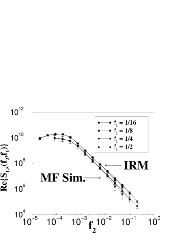
Figure 2: We present the $Re\{S_{1.5}(f_{2},f_{1})\}$ in the MF simulation and in the IRM. At high frequency $Re\{S_{1.5}(f_{2},f_{1})\}\sim f_{2}^{-V_{1.5}}$ (go to Table 1). There is not a visible flattening present due to $\Gamma_{1.5}^{(N)}(f_{1})$ ($\theta=0$) term, since the magnitude of this term is small relative to the $f_{2}$ dependent term.

The exponents $V_{1.5}$, $V_{2}$, $Q_{1.5}$, $Q_{2}$ are given in Table 1 for mean field theory, the IRM, and the experiment. Also, $A_{1.5}$, $A_{2}$, $B_{1.5}$, and $B_{2}$ are non-universal constants. In Eq. (25) and Eq. (28) $r=f_{a}/f_{b}$. Plots of Eqs. (26-28) are given in Figs. (2)-(4).

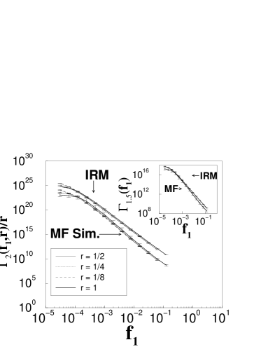
Figure 1: We present $\Gamma_{2}(f_{1},r)$ ($r=\frac{f_{a}}{f_{b}}=1$ corresponds to $\Gamma_{2}(f_{1})$, and we set $f_{1}=f_{b}$ for $r<1$) in the MF simulation and in the IRM. $\Gamma_{2}(f_{1},r)$ collapses for $r<1$, in excellent agreement with Eq. (25). For high frequency $\Gamma_{2}(f_{1},r)\sim f_{1}^{-Q_{2}}$, (see Table 1). Inset: $\Gamma_{1.5}(f_{1})$ for the MF and the IRM. For high frequency $\Gamma_{1.5}(f_{1})\sim f_{1}^{-Q_{1.5}}$, see Table 1.

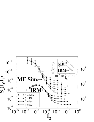
Figure 3: We present the $S_{2}(f_{2},f_{1})$ in the MF and IRM. Notice the flattening due to the $\Gamma_{2}^{(N)}(f_{1})$ ($\theta=0$) term. Inset: $S_{2}^{-}(f_{2},f_{1})$ is the second spectra in the MF simulation and the IRM with background term subtracted. The bold lines adjacent to the MF curve is a power law with an exponent of -2, and the bold line adjacent to the IRM curve has an exponent of -1.8.

The functions $\Gamma_{1.5}(f_{1})$, $\Gamma_{2}(f_{1})$, and $\Gamma_{2}(f_{b},r)$ are independent of $f_{2}$ since they resulted from the $\theta=0$ evaluation of $\langle v(t,f_{1})H(t+\theta,f_{1})\rangle$, $\langle H(t,f_{1})H(t+\theta,f_{1})\rangle$, and $\langle H(t_{a}+\theta,f_{a})H(t_{b},f_{b})\rangle$ (see Fig. 1). These $f_{2}$ independent terms are referred to as Gaussian background terms Seidler . Now $\Gamma_{1.5}^{(N)}(f_{1})$, $\Gamma_{2}^{(N)}(f_{1})$, and $\Gamma_{2}^{(N)}(f_{b},r)$ are $\Gamma_{1.5}(f_{1})$, $\Gamma_{2}(f_{1})$, and $\Gamma_{2}(f_{b},r)$ normalized by $\langle H(t,f_{1})\rangle_{t}$, $\langle H(t,f_{1})\rangle_{t}^{2}$, and $\langle H(t_{b},f_{b})\rangle_{t_{b}}\langle H(t_{a},f_{a})\rangle_{t_{a}}$, respectively. The first terms of Eq. (26) and Eq. (27) have no $f_{1}$ dependence, since the $f_{1}$ dependence of these terms drops out after they are normalized by $\langle H(t,f_{1})\rangle_{t}$ and $\langle H(t,f_{1})\rangle_{t}^{2}$, respectively. Nevertheless, the lack of $f_{1}$ dependence in the first terms of second spectra and real $1.5$ spectra is in excellent agreement with our simulation results, see Fig. 2 and the inset of Fig. 3. Also, we defer the discussion of $Im\{S_{2}(f_{2},f_{a},f_{b})\}$ and $Im\{S_{1.5}(f_{2},f_{1})\}$, since they are very sensitive to the non-stationary properties of the infinite avalanche in the analytical model. Please refer to Appendix C for details of how Eqs. (23-28) are calculated.

We present our results in Eq. (23-28) in terms of general scaling forms since the mean field and IRM simulations, as well as the experimental data, obey the same scaling form as mean field theory, only with different exponents and non-universal constants.

V SIMULATION

V.1 Mean Field Simulation

We perform $300$ runs of a simulation of the mean field RFIM. We collect data taken from $H\in[0,0.00125]$ at $R=0.79788$ ($R_{c}=0.79788456$) in systems with $N=15\times 10^{6}$ spins, and $J=1$. From this data we determine our simulation results agree with the scaling forms given in Eq. (23-28) with exponents given by Table 1. See Fig. 2-4.

V.2 Infinite Range Model Simulation

We perform $60$ runs of a 3D simulation of the IRM. The data was taken from $H\in[1.25,1.88]$ (from the slanted part of the hysteresis loop) at $R=2.2$ in system with $N=400^{3}$ spins, $J_{inf}=\frac{1}{N}$ and $J=1$. Again results agree with Eq. (23-28) with exponents given in Table 1. Refer to Fig. 2-4.

V.3 Finite Size Effects

We study finite size effects in our simulation (mean field and IRM) by examining higher order spectra for various system sizes. We find that for smaller system sizes the high frequency scaling (and flattening due to the background term) is unchanged for second spectra, real $1.5$ spectra, and real cross second spectra. However, at low frequency the scaling regime of the second spectra, real $1.5$ spectra, and real cross second spectra rolls over (in the IRM and MF simulations) at frequency $f_{1}\simeq\frac{1}{T_{max}}$, where $T_{max}$ is the maximum avalanche duration. $T_{max}$ is system size dependent where $T_{max}\sim L^{z}$, and $L=N^{1/d}$. In a $N=400^{3}$ system (IRM) we find that $T_{max}\simeq 4300$.

	$V_{1.5}$	$V_{2}$	$Q_{1.5}$	$Q_{2}$	$V_{C}$
MFT	2	2	3	5	2
MF Sim.	$1.93\pm 0.10$	$1.92\pm 0.12$	$2.95\pm 0.10$	$4.93\pm 0.12$	$1.92\pm 0.15$
IRM ($d=3$)	$1.80\pm 0.07$	$1.80\pm 0.05$	$2.73\pm 0.06$	$4.46\pm 0.07$	$1.82\pm 0.14$
Experiment	$0.93\pm 0.20$	$0.66\pm 0.12$	$2.81\pm 0.08$(h.f.)	$4.39\pm 0.15$(h.f.)	$0.63\pm 0.06$
			$1.66\pm 0.12$(l.f)	$2.48\pm 0.10$(l.f.)

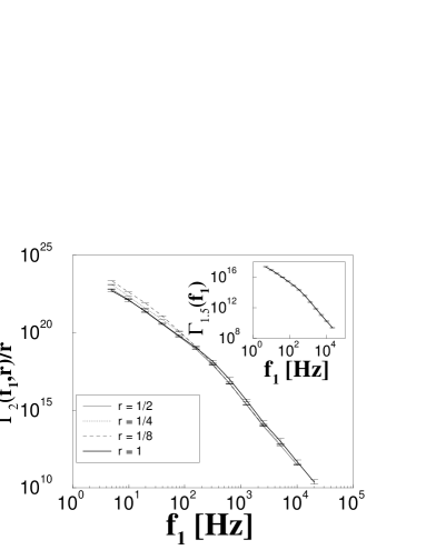
Figure 5: We present $\Gamma_{2}(f_{1},r)$ (where $r=\frac{f_{a}}{f_{b}}=1$ corresponds to $\Gamma_{2}(f_{1})$, and we set $f_{1}=f_{b}$ for $r<1$) in experiment. $\Gamma_{2}(f_{1},r)$ collapses for $r<1$, in excellent agreement with Eq. (25). For high frequency $\Gamma_{2}(f_{1},r)\sim f_{1}^{-Q_{2}}$, see Table 1. Inset: $\Gamma_{1.5}(f_{1})$ for experiment. For high frequency $\Gamma_{1.5}(f_{1})\sim f_{1}^{-Q_{1.5}}$, see Table 1.

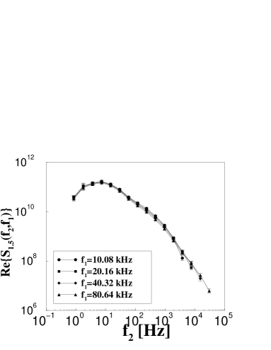
Figure 6: We present the real $1.5$ spectra $Re\{S_{1.5}(f_{2},f_{1})\}$ in experiment. At high frequency $Re\{S_{1.5}(f_{2},f_{1})\}\sim f_{2}^{-V_{1.5}}$ (go to Table 1). The high frequency scaling regime is small for the experimental real $1.5$ spectra since curve rolls over at $f_{cross}\simeq 320$ Hz.

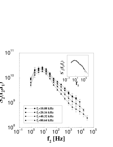
Figure 7: We present the second spectra, $S_{2}(f_{2},f_{1})$, in experiment. At high frequency the scaling is given $S_{2}(f_{2},f_{1})\sim f_{2}^{-V_{2}}$, where $V_{2}=0.66\pm 0.12$, that is significantly smaller than the mean field simulation ($V_{2}=1.92\pm 0.12$) and the IRM ($V_{2}=1.80\pm 0.05$). Further more, there is no conspicuous flattening in these experimental second spectra curves, indicating that the background term, $\Gamma_{2}^{(N)}(f_{1})$, is small for experiment versus the mean field simulation and the IRM. Also, there is a noticeable separation between curves at low frequency that is not present in the mean field simulation or IRM second spectra curves. Inset: $S_{2}^{-}(f_{2},f_{1})$ is the second spectra in experiment with the background term subtracted, as a result the seperation between the curves vanishes, within error bars.

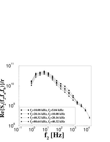
Figure 8: We present the real cross second spectra, $Re\{S_{2}(f_{2},f_{a},f_{b})\}$, for $r=f_{a}/f_{b}=\frac{1}{2}$, in experiment. Again, as in the experimental second spectra there is no conspicuous flattening due to the background term, $\Gamma_{2}^{(N)}(f_{b},r=\frac{1}{2})$. However, the seperation between the curves vanishes, within error bars, when the background term is subtrated off.

Table 1: We present the values of the exponents: $V_{1.5}$, $V_{2}$, $Q_{1.5}$, and $Q_{2}$ given in Eqs. (23-27) for mean field theory (MFT), mean field simulation (MF Sim.), the infinite range model (IRM) for $d=3$, and experiment. While the exponents values for MFT were determined analytically, the exponents for the MF Sim., IRM, and experiment were determined through a non-linear curve fitting of the data. In particular, in our experimental plots (Figs. 5-8) we use the following window sizes to fit the exponents: $f_{1}:[1kHz,200kHz]$ for $V_{1.5}$, $f_{1}:[20Hz,2kHz]$ for $V_{2}$, $f_{1}:[14kHz,40kHz]$ for $Q_{1.5}$ (high frequency exponent), $f_{1}:[.4kHz,18kHz]$ for $Q_{2}$ (high frequency exponent), and $f_{1}:[20Hz,2kHz]$ for $V_{C}$. We find that that these exponents do not change (outside of their error bars stated above) when the window size for their measurement is changed within the scaling regime of the data. Also, l.f. stands for low frequency and h.f. stands for high frequency, since for the experiment there are distinct l.f. and h.f. exponents, in some cases.

VI DISCUSSION

The mean field theoretical calculation was for a single infinite avalanche while the mean field simulation was obtained from a train of avalanches. Consequently, the train of avalanches introduces intermittency that lowers the magnitude of the mean field exponents, since the intermittency effectively adds white inter-avalanche noise to the intra-avalanche noise seen in the MF calculation. From Table 1 we notice that the exponents for our mean field simulation are systematically smaller (by an amount of $1\%$ to $4\%$) than the exponents determined in mean field theory. Nevertheless, despite this small deviate, our mean field simulation results agree very well with mean field theory, corroborating our theoretical calculation.

The background components ($\theta=0$), given by $\Gamma_{1.5}(f_{1})$ and $\Gamma_{2}(f_{b},r)$, are given in Fig. 1 for mean field theory and the mean field simulation. For the corresponding exponents $Q_{1.5}$ and $Q_{2}$ we find excellent agreement between mean field theory and the mean field simulation results. With the help of Dahmen we ascertain the following exponent relation for $Q_{2}$ and $Q_{1.5}$:

$$Q_{2}=\frac{5-\tau}{\sigma\nu z}-2$$ (29)

$$Q_{1.5}=\frac{1}{\sigma\nu z}+1$$ (30)

Plugging $\tau$ and $1/\sigma\nu z$ (given in Mehta ) into Eqs. (29-30) we find exact agreement in mean field theory: $Q_{2}=5$ and $Q_{1.5}=3$. For the IRM in $d=3$ we find $Q_{2}=4.40\pm 0.10$ and $Q_{1.5}=2.72\pm 0.03$, in close agreement with the table above. Also, for experiment we find reasonable agreement (within $10\%$) against the high frequency values for $Q_{2}$ and $Q_{1.5}$; using Eqs. (29-30) and Mehta we find $Q_{2}=2.70\pm 0.05$ and $Q_{1.5}=4.02\pm 0.20$ for experiment. Also, the measured experimental values for $Q_{2}$ and $Q_{1.5}$ in the table above agree within error bars with the exponents for the IRM.

Interestingly, we notice that the background components for experiment (given in Fig. 5) have two scaling regimes: a flatter slope at low frequency, a steeper slope at high frequency, and a transition point at $f_{cross}\simeq 320$ Hz. This change in slope indicates that intra-avalanche correlations are effecting the power at $f_{1}<f_{cross}$.

The real $1.5$ spectra and the second spectra are given in Figs. (2-3,6-7). Since the background term is small for the real $1.5$ spectra (for IRM, MF simulation, and experiment) we find that the real $1.5$ spectra curves collapse upon themselves, in agreement with Eq. (26). The high frequency scaling exponent $V_{1.5}$ for the real $1.5$ spectra shows excellent agreement between mean field theory ($V_{1.5}=2$) and mean field simulation ($V_{1.5}=1.93\pm 0.10$). The second spectra (Fig. 3) exhibits a conspicuous flattening due to the background term, except in the experimental second spectra (Fig. 7) where the flattening in much less pronounced. In order to find the high frequency scaling exponent for the second spectra we do a non-linear curve fit using the equation: $A0*x^{-A1}+$ (theoretical value, $\Gamma_{2}^{(N)}(f_{1})$), where $A0$, and $A1$, are free parameters. We find very good agreement between mean field theory ($V_{2}=2$) and our mean field simulation ($V_{2}=1.92\pm 0.12$) for our second spectra exponent.

The very weak dependence of the real $1.5$ spectra on $f_{1}$ and the strong fall off of the second spectra at high frequency suggests that the high frequency power comes from the fine structure of large avalanches ($T>>1/f_{1}$, $T$ is the duration) and not small individual pulses ($T\simeq 1/f_{1}$)Petta . Through simulation we verify this claim in the mean field simulation and IRM. When we subtract all avalanches smaller than $T=T_{max}/4$ from the Barkhausen train (where $T_{max}$ is the duration of the largest avalanche) and then determine the second spectra, we find no change in $V_{2}$. However, when we subtract all avalanches larger than $T=T_{max}/4$ from the Barkhausen train, we find that the second spectrum flattens and that there is an evident separation between the real $1.5$ spectra curves (i.e. increased $f_{1}$ dependence). In experiment we also find a weak dependence of the real $1.5$ spectra on $f_{1}$ and a strong fall off of the second spectra, however, the second spectra for experiment falls off with an exponent $V_{2}=0.66\pm 0.12$ versus an exponent of $V_{2}=1.80\pm 0.05$ for IRM and $V_{2}=2$ for mean field theory. This suggests that the high frequency power in experiment comes from the fine structure of larger pulses to a lesser degree than in IRM or mean field theory. This may be the result of dipole-dipole interactions that are present in experiment. Since the dipole-dipole interactions decay as a power law they may still be significant at short length scales, thereby resulting in suppressed spin flips that cause otherwise larger avalanches to be broken down in to smaller high frequency pulses. We are currently testing this hypothesis.

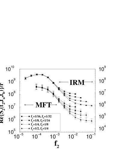
Figure 4: We present the $Re\{S_{2}(f_{2},f_{a},f_{b})\}$ for $r=f_{a}/f_{b}=\frac{1}{2}$ in the MF simulation and the IRM. Notice the flattening due to the $\Gamma_{2}^{(N)}(f_{b},r=\frac{1}{2})$ ($\theta=0$) term.

In Fig. 4 we give the real cross second spectra ($r=f_{a}/f_{b}=\frac{1}{2}$) for the mean field simulation and the IRM, and in Fig. 8 we give the real cross second spectra for experiment (also $r=\frac{1}{2}$). The cross second spectra plots for $r<\frac{1}{2}$ are similar to $r=\frac{1}{2}$, so to avoid redundancy $r<\frac{1}{2}$ plots have been left out of the paper. The real cross second spectra not only strongly resemble the second spectra, but we also notice in Table 1 that the exponents values for $V_{2}$ and $V_{C}$ (where $V_{C}$ was determined using the same non-linear curve fit used to find $V_{2}$) in mean field theory, the mean field simulation, the IRM, and in the experiment are identical or nearly identical. For the class of models and systems we study in this paper the real cross second spectra gives no new information, however, the real cross second spectra is useful when studying systems that have different dynamics on different length and time scales Weissman .

Remarkably, we have found that $Q_{1.5}$ and $Q_{2}$ agree (within error bars) for the IRM and experiment. Since $Q_{1.5}$ and $Q_{2}$ are directly related to known exponents, as we have found above, they may be obtained from a standard analysis of power spectra ($P(w)\sim w^{-\frac{1}{\sigma\nu z}}$) and the avalanche size distribution ($D(S)\sim S^{-\tau}$) Matt1 . However, when we compare $V_{1.5}$, $V_{2}$, and $V_{C}$ between the IRM and experiment we find a significant difference, whose origin we are currently investigating. Thus by utilizing higher order spectra we present a more rigorous test for avalanche models against experiment.

Our study of higher order spectra is a powerful tool to further our understanding of noise in disordered systems. In addition, our mean field results are applicable to a large array of systems, in particular systems discussed in Fisher .

Appendix A Calculation of Correlation functions

From Eq. (1) one can verify the following recursion relations:

$$<n_{j}> = <n_{j-1}>$$ (31)

$$<n_{j}^{2}> = <n_{j-1}^{2}>+<n_{j-1}>$$ (32)

$$<n_{j}^{3}> = <n_{j-1}^{3}>+3<n_{j-1}^{2}>+<n_{j-1}>$$ (33)

$$<n_{j}^{4}> = <n_{j-1}^{4}>+6<n_{j-1}^{3}>+7<n_{j-1}^{2}>+<n_{j-1}>$$ (34)

Using the fact that $n_{o}\equiv 1$ we determine the following initial conditions:

$$<n_{1}> = 1$$ (35)

$$<n_{1}^{2}> = 2$$ (36)

$$<n_{1}^{3}> = 5$$ (37)

$$<n_{1}^{4}> = 15$$ (38)

Using the recursion relations and initial conditions we can find the explicit functionality of $<n_{j}^{2}>$, $<n_{j}^{3}>$, and $<n_{j}^{4}>$:

$$<n_{j}^{2}> = <n_{j-1}^{2}>+<n_{j-1}>$$

$$= <n_{j-2}^{2}>+<n_{j-2}>+<n_{j-1}>$$

$$\ldots = <n_{1}^{2}>+\sum_{m=1}^{j-1}<n_{j-m}>$$

$$= 2+\sum_{m=1}^{j-1}1$$

$$= j+1$$

Thus we verify Eq. (4):

$$<n_{j}n_{j+k}>=<n_{j}^{2}>=j+1$$ (39)

Now let us consider:

$$<n_{j}^{3}> = <n_{j-1}^{3}>+3<n_{j-1}^{2}>+<n_{j-1}>$$

$$= <n_{j-2}^{3}>+3(<n_{j-2}^{2}>+<n_{j-1}^{2}>)+<n_{j-1}>+<n_{j-2}>$$

$$\ldots = <n_{1}^{3}>+3\sum_{m=1}^{j-1}<n_{j-m}^{2}>+\sum_{m=1}^{j-1}<n_{j-m}>$$

$$= 5+3\sum_{m=1}^{j-1}(j-m+1)+\sum_{m=1}^{j-1}1$$

$$= \frac{1}{2}(3j^{2}+5j+2)$$

Thus we find:

$$<n_{j}^{3}>=\frac{1}{2}(3j^{2}+5j+2)$$ (40)

Now let us find $<n_{j}^{4}>$:

$$<n_{j}^{4}> = <n_{j-1}^{4}>+6<n_{j-1}^{3}>+7<n_{j-1}^{2}>+<n_{j-1}>$$

$$= 15+\sum_{m=1}^{j-1}[6<n_{j-m}^{3}>+7<n_{j-m}^{2}>+<n_{j-m}>]$$

$$= \frac{1}{2}(6j^{3}+13j^{2}+9j+2)$$

So we have:

$$<n_{j}^{4}>=\frac{1}{2}(6j^{3}+13j^{2}+9j+2)$$ (41)

Now let us look at the case where $l\geq k\geq 0$:

$$<n_{j}n_{j+k}n_{j+l}> = <n_{i}n_{j+k}^{2}>$$

$$= <n_{j}(n_{j+k-1}+n_{j+k-1}^{2})>$$

$$= <n_{j}^{2}>+<n_{j}n_{j+k-1}^{2}>$$

$$= 2<n_{j}^{2}>+<n_{j}n_{j+k-2}^{2}>$$

$$\ldots$$

$$= k<n_{j}^{2}>+<n_{j}^{3}>$$

Thus:

$$<n_{j}n_{j+k}n_{j+l}>=<n_{j}^{3}>+k<n_{j}^{2}>$$ (42)

Now let’s look at the most general situation where $m\geq l\geq k\geq 0$:

$$<n_{j}n_{j+k}n_{j+l}n_{j+m}> = <n_{j}n_{j+k}n_{j+l}^{2}>$$

$$= <n_{j}n_{j+k}(n_{j+l-1}^{2}+n_{j+l-1})>$$

$$= <n_{j}n_{j+k}^{2}>+<n_{j}n_{j+k}n_{j+l-1}^{2}>$$

$$= <n_{j}n_{j+k}^{2}>+<n_{j}n_{j+k}(n_{j+l-2}^{2}+n_{j-l-2})>$$

$$= 2<n_{j}n_{j+k}^{2}>+<n_{j}n_{j+k}n_{j+l-2}^{2}>$$

$$\ldots$$

$$= (l-k)<n_{j}n_{j+k}^{2}>+<n_{j}n_{j+k}^{3}>$$

$$= (l-k)[<n_{j}^{3}>+k<n_{j}^{2}>]+<n_{j}n_{j+k}^{3}>$$

Now let’s determine $<n_{j}n_{j+k}^{3}>$:

$$<n_{j}n_{j+k}^{3}> = <n_{j}(n_{j+k-1}^{3}+3n_{j+k-1}^{2}+n_{j+k-1})>$$

$$= <n_{j}n_{j+k-1}^{3}>+3<n_{j}n_{j+k-1}^{2}>+<n_{j}n_{j+k-1}>$$

$$\ldots$$

$$= <n_{j}^{4}>+3\sum_{m=1}^{k-1}<n_{j}n_{j+m}^{2}>+k<n_{j}^{2}>$$

$$= <n_{j}^{4}>+3\sum_{m=1}^{k-1}[<n_{j}^{3}>+m<n_{j}^{2}>]+k<n_{j}^{2}>$$

$$= <n_{j}^{4}>+3k<n_{j}^{3}>+\frac{k}{2}(3k-1)<n_{j}^{2}>$$

Thus combining the above results we verify Eq. (7):

$$<n_{j}n_{j+k}n_{j+l}n_{j+m}>=<n_{j}^{4}>+(2k+l)<n_{j}^{3}>+\frac{k}{2}(k+2l-1)<n_{j}^{2}>$$ (43)

Appendix B Time Ordered products

In order to evaluate Eq. (11) we need to consider the time ordering of the indices of $n$, consider the following ($i<N$):

$$\tilde{y}=n_{1}+n_{2}+\ldots+n_{N-1}+n_{N}$$ (44)

$$x_{i}=n_{i}+n_{i+1}+\ldots+n_{N-1}+n_{N}$$ (45)

Now we want to evaluate $\tilde{y}^{2}$, $\tilde{y}^{3}$, $\tilde{y}^{4}$ we must write the expansion as a sum of time-ordered products, here’s how we do it:

$$\tilde{y}^{2}=(n_{1}+x_{2})^{2}=n_{1}^{2}+2n_{1}x_{2}+x_{2}^{2}$$ (46)

$$x_{2}^{2}=(n_{2}+x_{3})^{2}=n_{2}^{2}+2n_{2}x_{3}+x_{3}^{2}$$ (47)

$$x_{3}^{2}=(n_{3}+x_{4})^{2}=n_{3}^{2}+2n_{3}x_{4}+x_{4}^{2}$$ (48)

$$\ldots$$ (49)

Thus by we can write Eq. (46) as:

$$\tilde{y}^{2} = \sum_{i=1}^{N}[n_{i}^{2}+2n_{i}x_{i+1}]$$ (50)

$$= \sum_{i=1}^{N}[n_{i}^{2}+2n_{i}\sum_{j=i+1}^{N}n_{j}]$$ (51)

So we see that we have successfully written $\tilde{y}^{2}$ as a sum of time-ordered products. Now we can easily evaluate $<\tilde{y}^{2}>$ using Eqs. (3)-(4). This remarkable method can be used for higher powers to evaluate $\tilde{y}^{3}$, and $\tilde{y}^{4}$.

Appendix C Calculation of Higher Order Spectra

C.1 Second Spectra

We first rewrite the second spectra as the follows:

$$S_{2}(\omega,N)=\frac{\langle F_{i}\{H(i,N)\}F_{i}\{H(i,N)\}\rangle}{\langle H(i,N)\rangle_{i}^{2}}$$

$$=\frac{\sum\limits_{\theta=0}^{T/N-1}e^{2\pi i\theta\omega N/T}\sum\limits_{i=0}^{T/N-1-\theta}\langle H(i,N)H(i+\theta,N)\rangle}{\langle H(i,N)\rangle_{i}^{2}}$$

Where $i=t/N$, $\langle...\rangle_{i}$ denotes sum over $i$ ($\sum_{i=0}^{T/N-1}$), and $F_{i}\{..\}$ represents the discrete Fourier transform over $i$. The variable $\omega$ is conjugate variable to $i$ in the Fourier transform; $f_{2}=\omega/N$ is conjugate to $t$ (the original time) since $t=Ni$. We will use $\omega$ in subsequent calculations for consistency and do a change of variable to $f_{2}$ in our final expression. Also, we have set $\Delta t=1$.

Let’s first consider the second spectra, when $\theta>0$ we have:

$$\langle H(i+\theta,N)H(i,N)\rangle=\langle(\tilde{x}_{i+\theta}^{+}(N)-\tilde{x}_{i+\theta}^{-}(N))^{2}(\tilde{x}_{i}^{+}(N)-\tilde{x}_{i}^{-}(N))^{2}\rangle$$ (53)

This product is already partially time ordered since we know $\theta>0$, however when $\theta=0$:

$$\langle H(i,N)^{2}\rangle=\langle(\tilde{x}_{i}^{+}(N)-\tilde{x}_{i}^{-}(N))^{4}\rangle$$ (54)

In this case since $\theta=0$ no simplification can be made, there is no partial time ordering like in the case of Eq. (53).

We begin by evaluating Eq. (54), which can be written as a sum of 4-pt functions (Eq.(7)). To write Eq. (54) as a sum of 4-pt functions we must use the method discussed in Appendix B, which allows us to write any power of $\tilde{x}_{i}^{\pm}(N)$ as a sum of time ordered products in $n$:

$$\langle H(i,N)^{2}\rangle$$

$$=\langle(\tilde{x}_{i}^{+}-\tilde{x}_{i}^{-})^{4}\rangle$$

$$=\langle(\tilde{x}_{i}^{+})^{4}-4(\tilde{x}_{i}^{+})^{3}\tilde{x}_{i}^{-}+6(\tilde{x}_{i}^{+})^{2}(\tilde{x}_{i}^{-})^{2}-4\tilde{x}_{i}^{+}(\tilde{x}_{i}^{-})^{3}+(\tilde{x}_{i}^{-})^{4}\rangle$$

$$=\sum_{j=0}^{N/2-1}\Bigg{[}\Big{[}4(N/2-1-j)+1\Big{]}\langle n_{iN+j}^{4}\rangle+6\sum_{k=j+1}^{N/2-1}\Big{[}2(N/2-1-k)+1\Big{]}\langle n_{iN+j}^{2}n_{iN+k}^{2}\rangle$$

$$+4\sum_{k=j+1}^{N/2-1}\Big{[}(3(N/2-1-k)+1)\langle n_{iN+j}n_{iN+k}^{3}\rangle+3\sum_{l=k+1}^{N/2-1}(2(N/2-1-l)+1)\langle n_{iN+j}n_{iN+k}n_{iN+l}^{2}\rangle\Big{]}\Bigg{]}$$

$$-2N\sum_{j=0}^{N-1}\Bigg{[}\langle n_{iN+j}^{4}\rangle+\sum_{l=j+1}^{N/2-1}\Big{[}3\langle n_{iN+j}^{2}n_{iN+l}^{2}\rangle+3\langle n_{iN+j}n_{iN+l}^{3}\rangle+6\sum_{m=l+1}^{N/2-1}\langle n_{iN+j}n_{iN+l}n_{iN+m}^{2}\rangle\Big{]}\Bigg{]}$$

$$+6\sum_{j=0}^{N/2-1}\sum_{k=N/2}^{N-1}\Big{[}2(N-1-k)+1\Big{]}\Big{[}\langle n_{iN+j}^{2}n_{iN+k}^{2}\rangle+2\sum_{l=j+1}^{N/2-1}\langle n_{iN+j}n_{iN+l}n_{iN+k}^{2}\rangle\Big{]}$$

$$-4\sum_{j=0}^{N/2-1}\sum_{k=N/2}^{N-1}\Bigg{[}(3(N-1-k)+1)\langle n_{iN+j}n_{iN+k}^{3}\rangle+3\sum_{l=k+1}^{N-1}(2(N-1-l)+1)\langle n_{iN+j}n_{iN+k}n_{iN+l}^{2}\rangle\Bigg{]}$$

$$+\sum_{j=N/2}^{N-1}\Bigg{[}\Big{[}4(N/2-1-j)+1\Big{]}\langle n_{iN+j}^{4}\rangle+6\sum_{k=j+1}^{N-1}\Big{[}2(N/2-1-k)+1\Big{]}\langle n_{iN+j}^{2}n_{iN+k}^{2}\rangle$$

$$+4\sum_{k=j+1}^{N-1}\Big{[}(3(N-1-k)+1)\langle n_{iN+j}n_{iN+k}^{3}\rangle+3\sum_{l=k+1}^{N-1}(2(N-1-l)+1)\langle n_{iN+j}n_{iN+k}n_{iN+l}^{2}\rangle\Big{]}\Bigg{]}$$

Performing the above sum we find:

$$\langle H(i,N)^{2}\rangle$$ (55)

$$=\frac{N\left[64+56(21-20i)N^{2}-420N^{3}+14(58+80i)N^{4}-105N^{5}+4(61+70i)N^{6}\right]}{13440}$$ (56)

Finally summing over $i$ we obtain:

$$\Gamma_{2}(N)=\sum_{i=0}^{T/N-1}\langle H(i,N)^{2}\rangle$$ (57)

$$=\frac{1}{96}N(N^{2}+2)^{2}T^{2}+O(T)$$ (58)

$$\simeq\frac{1}{96}N^{5}T^{2}$$ (59)

Now let’s consider the case where $\theta>0$:

$$\langle H(i+\theta,N)H(i,N)\rangle$$

$$=\langle(\tilde{x}_{i}^{+}(N)-\tilde{x}_{i}^{-}(N))^{2}(\tilde{x}_{i+\theta}^{+}(N)-\tilde{x}_{i+\theta}^{-}(N))^{2}\rangle$$

$$=\Bigg{[}\sum_{l=0}^{N/2-1}\Big{[}2(N/2-1-l)+1-N\Big{]}+\sum_{l=N/2}^{N-1}\Big{[}2(N-1-l)+1\Big{]}\Bigg{]}\times$$

$$\Bigg{[}\sum_{j=0}^{N/2-1}\Big{[}2\sum_{k=j+1}^{N/2-1}\langle n_{iN+j}n_{iN+k}n_{(i+\theta)N+l}^{2}\rangle+\langle n_{iN+j}^{2}n_{(i+\theta)N+l}^{2}\rangle\Big{]}-2\sum_{j=0}^{N/2-1}\sum_{k=N/2}^{N-1}\langle n_{iN+j}n_{iN+k}n_{(i+\theta)N+l}^{2}\rangle$$

$$+\sum_{j=N/2}^{N-1}\Big{[}2\sum_{k=j+1}^{N-1}\langle n_{iN+j}n_{iN+k}n_{(i+\theta)N+l}^{2}\rangle+\langle n_{iN+j}^{2}n_{(i+\theta)N+l}^{2}\rangle\Big{]}\Bigg{]}$$

$$=\frac{1}{576}N^{3}(N^{2}+2)(5N^{2}+4+4i(N^{2}+2))$$

After summing over $i$ and performing Fourier transform we find:

$$\sum_{\theta=1}^{T/N-1}e^{2\pi i\theta\omega/T}\sum_{t=0}^{T/N-1-\theta}\langle H(t+\theta,N)H(t,N)\rangle$$

$$=\frac{N^{2}(N^{2}+2)^{2}T}{144\omega^{2}}$$

From Eq.(16) we know $\langle H(i,N)\rangle_{t}^{2}=\frac{T^{2}}{144}(N^{2}+2)^{2}$, also $f_{2}=\omega/N$, and $f_{1}=1/N$, so finally we obtain:

$$S_{2}(f_{2},f_{1})\simeq\frac{1}{Tf_{2}^{2}}+\frac{2}{3f_{1}}$$ (60)

C.2 $1.5$ Spectra

We first rewrite the $1.5$ spectra equation in a form we may analytically evaluate:

$$S_{1.5}(\omega,N)=\frac{\langle F_{i}\{v(i,N)\}F_{i}\{H(i,N)\}\rangle}{\langle H(i,N)\rangle_{i}}$$

$$=\frac{\sum\limits_{\theta=0}^{T/N-1}e^{2\pi i\theta\omega N/T}\sum\limits_{i=0}^{T/N-1-\theta}\langle v(i,N)H(i+\theta,N)\rangle}{\langle H(i,N)\rangle_{i}}$$

Where $v(i,N)\equiv\tilde{x}_{i}^{+}(N)+\tilde{x}_{i}^{-}(N)$. Now we consider the $1.5$ spectra, when $\theta=0$ we have:

$$\Gamma_{1.5}(N)=\sum_{i=0}^{T/N-1}\langle v(t,N)H(i,N)\rangle=\Big{[}\sum_{l=0}^{N/2-1}n_{iN+l}+\sum_{l=N/2}^{N-1}n_{iN+l}\Big{]}(\tilde{x}_{i}^{+}(N)-\tilde{x}_{i}^{-}(N))^{2}$$

$$=\sum_{i=0}^{T/N-1}\Bigg{[}\sum_{j=0}^{N/2-1}\Big{[}(3(N/2-1-j)+1)\langle n_{iN+j}^{3}\rangle+\sum_{k=j+1}^{N/2-1}3(2(N/2-1-k)+1)\langle n_{iN+j}^{2}n_{iN+k}\rangle\Big{]}$$

$$-N/2\sum_{j=0}^{N/2-1}\Big{[}\langle n_{iN+j}^{3}\rangle+2\sum_{k=j+1}^{N/2-1}\langle n_{iN+j}n_{iN+k}^{2}\rangle\Big{]}-\sum_{j=0}^{N/2-1}\sum_{k=N/2}^{N-1}\Big{[}2(N-1-k)\langle n_{iN+j}n_{iN+k}^{2}\rangle\Big{]}\Bigg{]}$$

$$=\frac{1}{24}N(N^{2}+2)T^{2}+O(T)$$

$$\simeq\frac{1}{24}N^{3}T^{2}$$

For the case $\theta>0$ we find:

$$\langle v(i,N)H(i+\theta,N)\rangle=\sum_{l=0}^{N-1}n_{iN+l}(\tilde{x}_{i+\theta}^{+}(N)-\tilde{x}_{i+\theta}^{-}(N))^{2}$$

$$=\sum_{l=0}^{N-1}\Bigg{[}\sum_{j=0}^{N/2-1}\Big{[}(2(N/2-1-j)+1-N\Big{]}\langle n_{iN+l}n_{(i+\theta)N+j}^{2}\rangle$$

$$+\sum_{j=N/2}^{N-1}\Big{[}2(N-1-j)+1\Big{]}\langle n_{iN+l}n_{(i+\theta)N+j}^{2}\rangle\Bigg{]}$$

$$=\frac{1}{24}N(N^{2}+2)(2Ni+N+1)$$

After summing over $i$, performing Fourier transform, and taking the real part we find:

$$Re\{\sum_{\theta=1}^{T/N-1}e^{2\pi i\theta\omega/T}\sum_{i=0}^{T/N-1-\theta}\langle v(i,N)H(i+\theta,N)\rangle\}$$

$$=\frac{N^{2}(N^{2}+2)T}{12\omega^{2}}$$

Now we normalize the result with $\langle H(i,N)\rangle_{t}=\frac{T}{12}(N^{2}+2)$, and substitute $f_{2}=\omega/N$, and $f_{1}=1/N$.

$$Re\{S_{1.5}(f_{2},f_{1})\}=\frac{1}{f_{2}^{2}}+\frac{f_{1}}{2}T$$ (61)

C.3 Cross Second Spectra

We rewrite the cross second spectra as follows:

$$S_{2}(\omega,M,N)=\frac{\langle F_{j}\{(j,M)\}F_{i}\{H(i,N)\}\rangle}{\langle H(i,N)\rangle_{i}\langle H(j,M)\rangle_{j}}$$

$$=\frac{\sum\limits_{\theta=0}^{T/N-1}e^{2\pi i\theta\omega N/T}\sum\limits_{i=0}^{T/N-1-\theta}\frac{M}{N}\sum\limits_{j=N(i-1)/M+1}^{Ni/M}\langle H(j,M)H(i+\theta,N)\rangle}{\langle H(i,N)\rangle_{i}\langle H(j,M)\rangle_{j}}$$

Where $M=\frac{1}{f_{b}}$, $N=\frac{1}{f_{a}}$, and $\langle...\rangle_{j}$ denotes sum over $j$ ($\sum_{j=0}^{T/M-1}$), Before we calculation of the cross second spectra we find it useful to define the following notation:

$$\tilde{y}^{-}_{j}(M)=\sum_{l=M/2}^{M-1}n_{Mj+l}$$

$$\tilde{y}^{+}_{j}(M)=\sum_{l=0}^{M/2-1}n_{Mj+l}$$

$$a=Ni/M$$

$$b=N(2i+1)/(2M)-1$$

$$c=N(i+1)/M-1$$

$$\tilde{x}^{-}_{i}(N)=\sum_{k=b+1}^{c}(\tilde{y}^{+}_{k}(M)+\tilde{y}^{-}_{k}(M))=\sum_{j=N/2}^{N-1}n_{Ni+j}$$

$$\tilde{x}^{+}_{i}(N)=\sum_{k=a}^{b}(\tilde{y}^{+}_{k}(M)+\tilde{y}^{-}_{k}(M))=\sum_{j=0}^{N/2-1}n_{Ni+j}$$

$$Y_{k}=\tilde{y}^{+}_{k}(M)+\tilde{y}^{-}_{k}(M)$$

$$X_{j}=\tilde{y}^{+}_{j}(M)-\tilde{y}^{-}_{j}(M)$$

Again first we consider case where $\theta=0$, using the notation above we have:

$$\Gamma_{2}(N,r)=\sum\limits_{i=0}^{T/N-1}\frac{M}{N}\sum\limits_{j=a}^{c}\langle H(j,M)H(i,N)\rangle$$ (62)

$$=\sum\limits_{i=0}^{T/N-1}\frac{M}{N}\sum\limits_{j=a}^{c}\langle(\tilde{y}_{j}^{+}(M)-\tilde{y}_{j}^{-}(M))^{2}(\tilde{x}_{i}^{+}(N)-\tilde{x}_{i}^{-}(N))^{2}\rangle$$ (63)

$$=\frac{M}{N}\sum\limits_{i=0}^{T/N-1}\sum\limits_{j=a}^{c}X_{j}^{2}\Big{[}\sum\limits_{j=a}^{b}Y_{k}-\sum\limits_{j=b+1}^{c}Y_{k}\Big{]}^{2}$$ (64)

$$=\frac{M}{N}\sum\limits_{i=0}^{T/N-1}\Big{[}\sum\limits_{j=a}^{b}X_{j}^{2}+\sum\limits_{j=b+1}^{c}X_{j}^{2}\Big{]}\Big{[}\sum\limits_{j=a}^{b}Y_{k}-\sum\limits_{j=b+1}^{c}Y_{k}\Big{]}^{2}$$ (65)

Now we make the follow approximation for Eq. (65), we simplify the limits by setting $N/M=2$ in the limits. By deduction this approximation will preserve the scaling for any $N/M$ (multiples of 2) in our final answer. Using $N/M=2$ to simplify the limits we find:

$$a=2i$$

$$b=2i$$

$$c=b+1=2i+1$$

We now expand Eq. (65):

$$\Gamma_{2}(N)=\frac{M}{N}\sum\limits_{i=0}^{T/N-1}\Big{(}X_{2i}^{2}+X_{2i+1}^{2}\Big{)}\Big{(}Y_{2i}-Y_{2i+1}\Big{)}^{2}$$

$$=\frac{M}{N}\sum\limits_{i=0}^{T/N-1}\Big{(}X_{2i}^{2}Y_{2i}^{2}+X_{2i+1}^{2}Y_{2i+1}^{2}+X_{2i+1}^{2}Y_{2i}^{2}+X_{2i}^{2}Y_{2i+1}^{2}-2X_{2i}^{2}Y_{2i}Y_{2i+1}-2X_{2i+1}^{2}Y_{2i+1}Y_{2i}\Big{)}$$

We evaluate the above terms below as a function of $k$, where $k$ represents either $2i$ or $2i+1$:

$$X_{k+1}^{2}Y_{k+1}Y_{k}$$

$$=\sum_{m=0}^{M-1}\sum_{q=M/2}^{M-1}\Bigg{[}\Big{[}3(M-1-q)+1\Big{]}\langle n_{kM+m}n_{(k+1)M+q}^{3}\rangle$$

$$+3\sum_{l=q+1}^{M-1}\Big{[}2(M-1-l)+1\Big{]}\langle n_{kM+m}n_{(k+1)M+q}n_{(k+1)M+l}^{2}\rangle\Bigg{]}$$

$$-\sum_{m=0}^{M-1}\sum_{l=M/2}^{M-1}\sum_{q=0}^{M/2-1}\Bigg{[}\Big{[}2(M-1-l)+1\Big{]}\langle n_{kM+m}n_{(k+1)M+q}n_{(k+1)M+l}^{2}\rangle\Bigg{]}$$

$$-M\sum_{m=0}^{M-1}\sum_{l=0}^{M/2-1}\Big{[}\langle n_{kM+m}n_{(k+1)M+l}^{3}\rangle+2\sum_{q=l+1}^{M/2-1}\langle n_{kM+m}n_{(k+1)M+l}n_{(k+1)M+q}^{2}\rangle\Big{]}$$

$$+\sum_{m=0}^{M-1}\sum_{q=0}^{M/2-1}\Bigg{[}\Big{[}3(M/2-1-q)+1\Big{]}\langle n_{kM+m}n_{(k+1)M+q}^{3}\rangle$$

$$+3\sum_{l=q+1}^{M/2-1}\Big{[}2(M/2-1-l)+1\Big{]}\langle n_{kM+m}n_{(k+1)M+q}n_{(k+1)M+l}^{2}\rangle\Bigg{]}$$

$$X_{k+1}^{2}Y_{k}^{2}$$

$$=\Bigg{[}\sum_{m=0}^{M/2-1}\Big{[}2(M/2-1-m)+1-M\Big{]}+\sum_{m=M/2}^{M-1}\Big{[}2(M-1-m)+1\Big{]}\Bigg{]}$$

$$\times\Big{[}\sum_{n=0}^{M-1}\Big{(}\langle n_{kM+n}^{2}n_{(k+1)M+m}^{2}\rangle+2\sum_{l=n+1}^{M-1}\langle n_{kM+n}n_{kM+l}n_{(k+1)M+n}^{2}\rangle\Big{)}\Big{]}$$

$$X_{k}^{2}Y_{k}^{2}$$

$$=\sum_{j=M/2}^{M-1}\Bigg{[}\Big{[}4(M-1-j)+1\Big{]}\langle n_{Mk+j}^{4}\rangle$$

$$+6\sum_{m=j+1}^{M-1}\Big{[}2(M-1-m)+1\Big{]}\langle n_{Mk+j}^{2}n_{Mk+m}^{2}\rangle$$

$$+\sum_{m=j+1}^{M-1}4\Big{[}\Big{(}3(M-1-m)+1\Big{)}\langle n_{Mk+j}n_{Mk+m}^{3}\rangle$$

$$+\sum_{l=m+1}^{M-1}3\Big{(}2(M-1-l)+1\Big{)}\langle n_{Mk+j}n_{Mk+m}n_{Mk+l}^{2}\rangle\Big{]}\Bigg{]}$$

$$-2\sum_{j=0}^{M/2-1}\sum_{m=M/2}^{M-1}\Big{[}2(M-1-m)+1\Big{]}\times\Big{[}\langle n_{Mk+j}^{2}n_{Mk+m}^{2}\rangle+\sum_{l=j+1}^{M/2-1}2\langle n_{Mk+j}n_{Mk+l}n_{Mk+m}^{2}\rangle\Big{]}+$$

$$\sum_{j=0}^{M/2-1}\Bigg{[}\Big{[}4(M/2-1-j)+1\Big{]}\langle n_{Mk+j}^{4}\rangle$$

$$+6\sum_{m=j+1}^{M/2-1}\Big{[}2(M/2-1-m)+1\Big{]}\langle n_{Mk+j}^{2}n_{Mk+m}^{2}\rangle$$

$$+\sum_{m=j+1}^{M/2-1}4\Big{[}\Big{(}3(M/2-1-m)+1\Big{)}\langle n_{Mk+j}n_{Mk+m}^{3}\rangle$$

$$+\sum_{l=m+1}^{M/2-1}3\Big{(}2(M/2-1-l)+1\Big{)}\langle n_{Mk+j}n_{Mk+m}n_{Mk+l}^{2}\rangle\Big{]}\Bigg{]}$$

$$X_{k}^{2}Y_{k}Y_{k+1}$$

$$=M\sum_{m=M/2}^{M-1}\Bigg{[}\langle n_{kM+m}^{4}\rangle+3\sum_{l=m+1}^{M-1}\langle n_{kM+m}^{2}n_{kM+l}^{2}\rangle$$

$$+3\sum_{l=m+1}^{M-1}\Big{[}\langle n_{kM+m}n_{kM+l}^{3}\rangle+2\sum_{q=l+1}^{M-1}\langle n_{kM+m}n_{kM+l}n_{kM+q}^{2}\rangle\Big{]}\Bigg{]}$$

$$-M\sum_{m=0}^{M/2-1}\sum_{l=M/2}^{M-1}\Big{[}\langle n_{kM+m}n_{kM+l}^{3}\rangle+2\sum_{q=l+1}^{M-1}\langle n_{kM+m}n_{kM+l}n_{kM+q}^{2}\rangle\Big{]}$$

$$-M\sum_{m=0}^{M/2-1}\sum_{l=M/2}^{M-1}\Big{[}\langle n_{kM+m}^{2}n_{kM+l}^{2}\rangle+2\sum_{q=m+1}^{M-1}\langle n_{kM+m}n_{kM+q}n_{kM+l}^{2}\rangle\Big{]}$$

$$+M\sum_{m=0}^{M/2-1}\Bigg{[}\langle n_{kM+m}^{4}\rangle+3\sum_{l=m+1}^{M/2-1}\langle n_{kM+m}^{2}n_{kM+l}^{2}\rangle$$

$$+3\sum_{l=m+1}^{M/2-1}\Big{[}\langle n_{kM+m}n_{kM+l}^{3}\rangle+2\sum_{q=l+1}^{M/2-1}\langle n_{kM+m}n_{kM+l}n_{kM+q}^{2}\rangle\Big{]}\Bigg{]}$$

$$X_{k}^{2}Y_{k+1}^{2}=\sum_{n=0}^{M-1}\Big{[}2(M-1-n)+1\Big{]}$$

$$\times\Bigg{[}\sum_{n=0}^{M-1}\sum_{m=M/2}^{M-1}\Big{(}\langle n_{kM+m}^{2}n_{(k+1)M+n}^{2}\rangle+2\sum_{l=m+1}^{M-1}\langle n_{kM+m}n_{kM+l}n_{(k+1)M+n}^{2}\rangle\Big{)}$$

$$-2\sum_{m=0}^{M/2-1}\sum_{l=M/2}^{M-1}\langle n_{kM+m}n_{kM+l}n_{(k+1)M+n}^{2}\rangle+$$

$$\sum_{m=0}^{M/2-1}\Big{(}\langle n_{kM+m}^{2}n_{(k+1)M+n}^{2}\rangle+2\sum_{l=m+1}^{M-1}\langle n_{kM+m}n_{kM+l}n_{(k+1)M+n}^{2}\rangle\Big{)}\Bigg{]}$$

Now we can evaluate Eq. (65) (where $r=M/N$):

$$\Gamma_{2}(N,r)=\frac{M^{5}r^{3}}{144}\Big{(}5+\frac{4}{M^{3}}\Big{)}T^{2}\simeq\frac{25M^{5}r^{3}}{144}T^{2}$$ (66)

The $\theta>0$ case is readily evaluated as followed:

$$\langle H(j,M)H(i+\theta,N)\rangle=\langle(\tilde{y}^{+}_{j}-\tilde{y}^{-}_{j})^{2}(\tilde{x}^{+}_{i+\theta}-\tilde{x}^{-}_{i+\theta})^{2}\rangle$$

$$=\Bigg{[}\sum_{l=0}^{M/2-1}\Big{[}2(N/2-1-l)+1-N\Big{]}+\sum_{l=M/2}^{M-1}\Big{[}2(N-1-l)+1\Big{]}\Bigg{]}$$

$$\times\Bigg{[}\sum_{m=0}^{M/2-1}\Big{[}2\sum_{k=m+1}^{M/2-1}\langle n_{jM+m}n_{jM+k}n_{(i+\theta)N+l}^{2}\rangle+\langle n_{jM+m}^{2}n_{(i+\theta)N+l}^{2}\rangle\Big{]}$$

$$-2\sum_{m=0}^{M/2-1}\sum_{k=M/2}^{M-1}\langle n_{jM+n}n_{jM+k}n_{(i+\theta)N+l}^{2}\rangle$$

$$+\sum_{m=M/2}^{M-1}\Big{[}2\sum_{k=m+1}^{M-1}\langle n_{jM+m}n_{jM+k}n_{(i+\theta)N+l}^{2}\rangle+\langle n_{jM+m}^{2}n_{(i+\theta)N+l}^{2}\rangle\Big{]}\Bigg{]}$$

After summing over $i$ and performing Fourier transform and taking the real part we find:

$$Re\{\sum_{\theta=1}^{T/N-1}e^{2\pi i\theta\omega/T}\sum_{i=0}^{T/N-1-\theta}\langle H(j,M)H(i+\theta,N)\rangle\}$$

$$=\frac{MN(M^{2}+2)(N^{2}+2)T}{144\omega^{2}}$$

From Eq.(16) we know $\langle H(i,N)\rangle_{t}\langle H(j,M)\rangle_{t}=\frac{T^{2}}{144}(N^{2}+2)(M^{2}+2)$, $f_{2}=\omega/N$, $f_{a}=1/N$, and $f_{b}=1/M$ finally we obtain:

$$Re\{S_{2}(f_{2},f_{a},f_{b})\}\simeq\frac{r}{Tf_{2}^{2}}+\frac{25r^{5}}{f_{a}}$$ (67)

References

- (1) J.P. Sethna, K. A. Dahmen, and C.R. Myers, Crackling Noise, Nature 410, 242 (2001).
- (2) Matthew C. Kuntz, and James P. Sethna, Phys. Rev. B 62, 11699 (2000).
- (3) D.S. Fisher, Phys. Reports 301, 113 (1998).
- (4) K.P. O’Brien and M.B. Weissman, Phys. Rev. E 50(5), 3446 (1994); K.P. O’Brien and M.B. Weissman, Phys. Rev. A 46(8), R4475 (1992)
- (5) J.R. Petta, M.B. Weissman, and G. Durin, Phys. Rev. E 57(6), 6363 (1998).
- (6) R.D. Merithew, M.W. Rabin, M.B. Weissman, M.J. Higgins, and S.Bhattacharya, Phys. Rev. Lett. 77(15), 3197 (1996).
- (7) M.G.A. Thomson, Phys. Rev. Lett. 86(13), 2901 (2001).
- (8) C.E. Parman, N.E. Israeloff, and J. Kakalios, Phys. Rev. Lett. 69(7), 1097 (1992).
- (9) G.T. Seidler, and S.A. Solin, Phys. Rev. B 53(15), 9753 (1996).
- (10) M.B. Weissman, Annu. Rev. Mater. Sci. 26, 395 (1996).
- (11) K. A. Dahmen, Hysteresis, Avalanches, and Disorder Induced Critical Scaling: A Renormalization Group Approach, Ph.D. Thesis, Cornell University (May 1995); K. Dahmen, and J. P. Sethna, Phys. Rev. B 53, 14872 (1996).
- (12) J.S. Urbach, R.C. Madison, and J.T. Markert, Phys. Rev. Lett. 75(2), 276 (1995).
- (13) O. Narayan, Phys. Rev. Lett. 77(18), 3855 (1996).
- (14) S. Zapperi, P. Cizeau, G. Durin, and H.E. Stanley, Phys. Rev. B 58(10), 6353 (1998).
- (15) Matthew C. Kuntz, Olga Perković, Karin A. Dahmen, Bruce W. Roberts, and James P. Sethna, Comput. Sci. Eng. 1, 73 (1999).
- (16) James P. Sethna, Olga Perković, and Karin A. Dahmen, preprint (1997), Los Alamos Nat’l Laboratory Archive, http://xxx.lanl.gov/abs/cond-mat/9704059.
- (17) B. Alessandro, C. Beatrice, G. Bertotti, and A. Montorsi, J. Appl. Phys. 68, 2901 (1990).
- (18) Amit P. Mehta, Andrea C. Mills, Karin Dahmen, and James P. Sethna, Phys. Rev. E 65, 46139 (2002).