A basis for the statistical mechanics of granular systems

Abstract

This paper aims to justify the use of statistical mechanics tools in situations where the system is out of equilibrium and jammed. Specifically, we derive a Boltzmann equation for a jammed granular system and show that the Boltzmann’s analysis can be used to produce a “Second Law”, $\dot{S}\geq 0$ for jammed systems. We highlight the fundamental questions in this area of physics and point to the key quantities in characterising a packing of particles, accessible through a novel experimentation method which we also present here.

1 Introduction

In a thermal system, the Brownian motion of the constituent particles implies that the system dynamically explores the available energy landscape, such that the notion of a statistical ensemble applies. For densely packed systems of interest in this study, in which enduring contacts between particles are important, the potential energy barrier prohibits an equivalent random motion. At first sight it seems that the thermal statistical mechanics do not apply to these systems as there is no mechanism for averaging over the configurational states. Hence, these systems are inherently out of equilibrium. On the other hand, if the granular material is gently tapped such that the grains can slowly explore the available configurations, the situation becomes analogous to the equilibrium case scenario. It has been shown that the volume of the system is dependent on the applied tapping regime, and that this dependence is reversible, implying ergodicity [1]. This result gives support to the proposed statistical ensemble valid for dense, static and slowly moving granular materials which was first introduced by Edwards and Oakeshott in 1989 [2, 3]. Through this approach, notions of macroscopic quantities such as entropy and compactivity were also introduced to granular matter.

Here we present a theoretical framework to fully describe the exact specificities of granular packings, and a shaking scenario which leads to the derivation of the Boltzmann equation for a jammed granular system. This kind of an analysis paves the path to the study of macroscopic quantities, such as the compactivity, characterising each jammed configuration from the microstructural information of the packing. It is according to this theory that the static configurations obtained from experiments are later characterised. An extended version of this paper is presented in [4].

2 Classical Statistical Mechanics

We first present the classical statistical mechanics theorems to an extent which facilitates an understanding of the important concepts for the development of an analogous granular theory, as well as the assumptions necessary for the belief in such a parallel approach. In the conventional statistical mechanics of thermal systems, the different possible configurations, or microstates, of the system are given by points in the phase space of all positions and momenta {$p,q$} of the constituent particles. The equilibrium probability density $\rho_{\mbox{\scriptsize eqm}}$ must be a stationary state of Liouville’s equation which implies that $\rho_{\mbox{\scriptsize eqm}}$ must be expressed only in terms of the total energy of the system, $E$. The simplest form for a system with Hamiltonian ${\cal H}(p,q)$ is the microcanonical distribution:

$$\rho_{\mbox{\scriptsize eqm}}(E)=\frac{1}{\Sigma_{\mbox{\scriptsize eqm}}(E)},$$ (1)

for the microstates within the ensemble, ${\cal H}(p,q)=E$, and zero otherwise. Here,

$$\Sigma_{\mbox{\scriptsize eqm}}(E)=\int\delta(E-{\cal H}(p,q))~{}~{}dp~{}dq,$$ (2)

is the area of energy surface ${\cal H}(p,q)=E$.

Equation (1) states that all microstates are equally probable. Assuming that this is the true distribution of the system implies accepting the ergodic hypothesis, i.e. the trajectory of the closed system will pass arbitrarily close to any point in phase space.

It was the remarkable step of Boltzmann to associate this statistical concept of the number of microstates with the thermodynamic notion of entropy through his famous formula

$$S_{\mbox{\scriptsize eqm}}(E)=k_{B}\log\Omega{\mbox{\scriptsize eqm}}(E).$$ (3)

Whereas the study of thermal systems has had the advantage of available statistical mechanics tools for the exploration of the phase space, an entirely new statistical method, unrelated to the temperature, had to be constructed for grains.

3 Statistical Mechanics for Jammed Matter

We now consider a jammed granular system composed of rigid grains. Such a system is analogously described by a network of contacts between the constituent particles in a fixed volume $V$, since there is no relevant energy $E$ in the system. In the case of granular materials, the analogue of phase space, the space of microstates of the system, is the space of possible jammed configurations as a function of the degrees of freedom of the system $\{\zeta\}$.

It is argued that it is the volume of this system, rather than the energy, which is the key macroscopic quantity governing the behaviour of granular matter [2, 3]. If we have $N$ grains of specified shape which are assumed to be infinitely rigid, the system’s statistics would be defined by a volume function ${\cal W}(\zeta)$, a function which gives the volume of the system in terms of the specification of the grains.

In this analogy one replaces the Hamiltonian ${\cal H}(p,q)$ of the system by the volume function, ${\cal W}(\zeta)$. The average of ${\cal W}(\zeta)$ over all the jammed configurations determines the volume $V$ of the system in the same way as the average of the Hamiltonian determines the average energy $E$ of the system.

3.1 Definition of the volume function, $\cal W$

One of the key questions in this analogy is to establish the ‘correct’ $\cal W$ function, the statistics of which is capable of fully describing the system as a whole. The idea is to partition the volume of the system into different subsystems, $\alpha$ with volume ${\cal W}^{\alpha}$, such that the total volume of a particular configuration is

$${\cal W}(\zeta)=\sum_{\alpha}{\cal W}^{\alpha}$$ (4)

It could be that considering the volume of the first coordination shell of particles around each grain is sufficient; thus, we may identify the partition $\alpha$ with each grain. However, particles further away may also play a role in the collective system response due to enduring contacts, in which case $\cal W$ should encompass further coordination shells. In reality, of course, the collective nature of the system induces contributions from grains which are indeed further away from the grain in question, but the consideration of only its nearest neighbours is a good starting point for solving the system, and is the way in which we proceed to describe the $\cal W$ function. The significance of the appropriate definition of $\cal W$ is best understood by the consideration of a response to an external perturbation to the system in terms of analogies with the Boltzmann equation which we will describe in Section 5.

Ball and Blumenfeld [5] have shown by a triangulation method that the area of the two-dimensional problem can be given in terms of the contact points using vectors constructed from them. Here we consider a cruder version for the volume per grain, yet with a strong physical meaning. For a pair of grains in contact (assumed to be point contacts for rough, rigid grains) the grains are labelled $\alpha,\beta$, and the vector from the centre of $\alpha$ to that of $\beta$ is denoted as ${\rm\bf R}^{\,\alpha\beta}$ and specifies the complete geometrical information of the packing. The first step is to construct a configurational tensor ${\rm\bf\cal C}^{\alpha}$ associated with each grain $\alpha$ based on the structural information,

$${\cal C}_{ij}^{\alpha}=\sum_{\beta}R_{i}^{\alpha\beta}R_{j}^{\alpha\beta}.$$ (5)

Then an approximation for the area in 2D or volume in 3D encompassing the first coordination shell of the grain in question is given as

$${\cal W}^{\alpha}=2\sqrt{\mbox{Det}{\cal C}_{ij}^{\alpha}}.$$ (6)

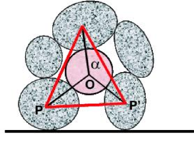
Figure 1: Volume function $\cal W$ as discussed in the text.

The volume function is depicted in the Fig. 1, with grain coordination number 3 in two dimensions, where Eq. (6) should give the area of the triangle (thick gray lines) constructed by the centres $P$ of grains which are in contact with the $\alpha$ grain. The above equation is exact if the area is considered as the determinant of the vector cross product matrix of the two sides of the triangle. However, this definition is clearly only an approximation of the space available to each grain since there is an overlap of ${\cal W}^{\alpha}$ for grains belonging to the same coordination shell. Thus, it overestimates the total volume of the system: $\sum{\cal W}^{\alpha}>V$. However, it is the simplest approximation for the system based on a single coordination shell of a grain.

3.2 Entropy and compactivity

Now that we have explicitly defined $\cal W$ it is possible to define the entropy of the granular packing. The number of microstates for a given volume $V$ is measured by the area of the surface ${\cal W}(\zeta)=V$ in the phase space of jammed configurations and it is given by:

$$\Sigma_{\mbox{\scriptsize jammed}}(V)=\int\delta\Big{(}V-{\cal W}(\zeta)\Big{)}~{}~{}\Theta(\zeta)~{}~{}d\zeta,$$ (7)

where now $d\zeta$ refers to an integral over all possible jammed configurations and $\delta(V-{\cal W}(\zeta))$ formally imposes the constraint to the states in the sub-space ${\cal W}(\zeta)=V$. $\Theta(\zeta)$ is a constraint that restricts the summation to only reversible jammed configurations [4]. The radical step is the assumption of equally probable microstates which leads to an analogous thermodynamic entropy associated with this statistical quantity:

$$S(V)=\lambda\log\Sigma_{\mbox{\scriptsize jammed}}(V)=\lambda\log\int\delta(V-{\cal W}(\zeta))~{}~{}\Theta(\zeta)~{}~{}d\zeta,$$ (8)

which governs the macroscopic behaviour of the system [2, 3]. Here $\lambda$ plays the role of the Boltzmann constant. The corresponding analogue of temperature, named the “compactivity”, is defined as

$$X^{-1}=\frac{{\partial S}}{{\partial V}}.$$ (9)

This is a bold statement, which perhaps requires further explanation in terms of the actual role of compactivity in describing granular systems. We can think of the compactivity as a measure of how much more compact the system could be, i.e. a large compactivity implies a loose configuration (e.g. random loose packing, RLP) while a reduced compactivity implies a more compact structure (e.g. random close packing, RCP). In terms of the reversible branch of the compaction curve obtained in the Chicago experiments [1] large amplitudes generate packings of high compactivities, while in the limit of the amplitude going to zero a low compactivity is achieved. In terms of the entropy, many more configurations are available at high compactivity, thus the dependence of the entropy on the volume fraction can be qualitatively described as in Fig. 2. In the figure, for monodisperse packings the RCP is identified at $\phi\approx 0.64$, the maximum RLP fraction is identified at $\phi\approx 0.59$, while the crystalline packing, FCC, is at $\phi=0.74$ but cannot be reached by tapping.

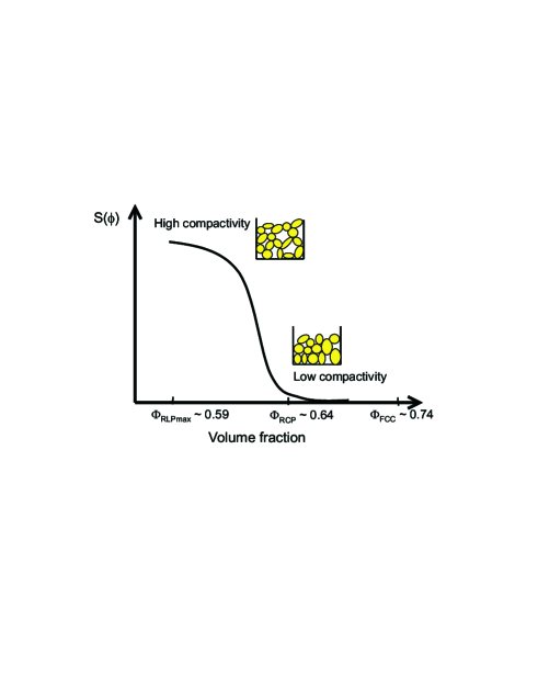
Figure 2: Interpretation of the compactivity and entropy in terms of different packings.

3.3 Remarks

To summarise, the granular thermodynamics is based on two postulates:

1) While in the Gibbs construction one assumes that the physical quantities are obtained as an average over all possible configurations at a given energy, the granular ensemble consists of only the jammed configurations at the appropriate volume.

2) As in the microcanonical equilibrium ensemble, the strong ergodic hypothesis is that all jammed configurations of a given volume can be taken to have equal statistical probabilities.

The ergodic hypothesis for granular matter was treated with skepticism, mainly because a real powder bears knowledge of its formation and the experiments are therefore history dependent. Thus, any problem in soil mechanics or even a controlled pouring of a sand pile does not satisfy the condition of all jammed states being accessible to one another as ergodicity has not been achieved, and the thermodynamic picture is therefore not valid. However the Chicago experiments of tapping columns [1] showed the existence of reversible situations. For instance, let the volume of the column be $V(n,\Gamma)$ where $n$ is the number of taps and $\Gamma$ is the strength of the tap. If one first obtain a volume $V(n_{1},\Gamma_{1})$, and then repeat the experiment at a different tap intensity and obtain $V(n_{2},\Gamma_{2})$, when we return to tapping at $(n_{1},\Gamma_{1})$ one obtains a volume $V^{\prime}$ which is $V^{\prime}(n_{1},\Gamma_{1})=V(n_{1},\Gamma_{1})$. There have been several further experiments confirming these results for different system geometries, particle elasticities and compaction techniques, e. g. the system can be mechanically tapped or oscillated, vibrated using a loudspeaker, or even allowed to relax under large pressures over long periods of time, all to the same effect [6, 7, 8]. Moreover, in simulations of slowly sheared granular systems the ergodic hypothesis was shown to work [9].

It is often noted in the literature that although the simple concept of summing over all jammed states which occupy a volume $V$ works, there is no first principle derivation of the probability distribution of the granular ensemble as it is provided by Liouville’s theorem for equilibrium statistical mechanics of liquids and gases. In granular thermodynamics there is no justification for the use of the $\cal W$ function to describe the system as Liouville’s theorem justifies the use of the energy in the microcanonical ensemble. In Section 5 we will provide an intuitive proof for the use of $\cal W$ in granular thermodynamics by the analogous proof of the Boltzmann equation.

The comment was nevertheless made that there is no proof that the entropy Eq. (8) is a rigorous basis for granular statistical mechanics. Here we develop a Boltzmann equation for jammed systems and show that this analysis can be used to produce a second law of thermodynamics, $\delta S\geq 0$ for granular matter, and the equality only comes with Eq. (8) being achieved. Although everyone believes that the second law of thermodynamics is universally true in thermal systems, the only accessible proof comes in the Boltzmann equation, as the ergodic theory is a difficult branch of mathematics which will not be covered in the present discussion. By investigating the assumptions and key points which led to the derivation of the Boltzmann equation in thermal systems, it is possible to draw analogies for an equivalent derivation in jammed systems.

It should be noted that there is an extensive literature on granular gases [10, 11], which are observed when particles are fluidised by vigorous shaking, thus inducing continuous particle collisions. There is a powerful literature on this topic, but it is not applicable to the problem of jamming.

4 The Classical Boltzmann Equation

The notion of entropy is important for thermal systems because it satisfies the second law,

$$\frac{\partial S}{\partial t}\geq 0,$$ (10)

which states that there is a maximum entropy state which, according to the evolution in Eq. (10), any system evolves toward, and reaches at equilibrium. A semi-rigorous proof of the Second Law was provided by Boltzmann (the well-known ‘H-theorem’), by making use of the ‘classical Boltzmann equation’, as it is now known.

In order to derive this equation, Boltzmann made a number of assumptions concerning the interactions of particles. The most important of these assumptions were:

• The collision processes are dominated by two-body collisions (Fig. 3a). This is a plausible assumption for a dilute gas since the system is of very low density, and the probability of there being three or more particles colliding is infinitesimal.

• Collision processes are uncorrelated, i.e. all memory of the collision is lost on completion and is not remembered in subsequent collisions: the famous Stosszahlansatz. This is also valid only for dilute gases, but the proof is more subtle.

Thus, Boltzmann proves Eq. (10) for a dilute gas only, but this is a readily available situation. The remaining assumptions have to do with the kinematics of particle collisions, i.e. conservation of kinetic energy, conservation of momentum, and certain symmetry of the particle scattering cross-sections.

Let $f(v,r)$ denote the probability of a particle having a velocity $v$ at position $r$. This probability changes in time by virtue of the collisions. The two particle collision is visualised in Fig. 3a where $v$ and $v_{1}$ are the velocities of the particles before the collision and $v^{\prime}$ and $v^{\prime}_{1}$ after the collision.

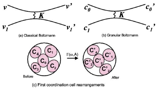
Figure 3: (a) Collision of two particles in a dilute gas. (b) “Collision of two configurations” given in terms of two contact points in a jammed material. (c) Rearrangements inside a pocket ${\it a}$ under the first coordination shell approximation of grain $\alpha=0$.

On time scales larger than the collision time, momentum and kinetic energy conservation apply:

$$mv+mv_{1}=mv^{\prime}+mv_{1}^{\prime},\\ \\ \\ \\ \\ \\ \\ \\ \\ \ \frac{1}{2}mv^{2}+\frac{1}{2}mv_{1}^{2}=\frac{1}{2}mv^{\prime 2}+\frac{1}{2}m{v^{\prime}}_{1}^{2}.$$ (11)

Then, the distribution $f(v,r)$ evolves with time according to

$$\frac{\partial f}{\partial t}+v\frac{\partial f}{\partial r}+\int{\cal K}(v,v^{\prime};v_{1},v_{1}^{\prime})~{}~{}\Big{(}f(v)f(v_{1})-f(v^{\prime})f(v_{1}^{\prime})\Big{)}~{}~{}d^{3}v_{1}d^{3}v^{\prime}d^{3}v_{1}^{\prime}=0.$$ (12)

The kernel $\cal K$ is positive definite and contains $\delta$-functions to satisfy the conditions (11), the flux of particles into the collision and the differential scattering cross-section. We consider the case of homogeneous systems, i.e. $f=f(v)$, and define

$$S=-k_{B}\int f\log f.$$ (13)

Defining $x=ff_{1}/f^{\prime}f^{\prime}_{1}$ we obtain

$$\frac{\partial S}{\partial t}=\int{\cal K}~{}\log x~{}(1-x)d^{3}v_{1}~{}d^{3}v^{\prime}~{}d^{3}v_{1}^{\prime},\\ (1-x)\log x\geq 0,\\ {\cal K}\geq 0.$$ (14)

Hence $\partial S/\partial t\geq 0$ (see standard text books on statistical mechanics).

It is also straightforward to establish the equilibrium distribution where $\partial S/\partial t=0$ since it occurs when the kernel term vanishes. This occurs when the condition of detailed balance is achieved, $x=1$:

$$f(v)f(v_{1})=f(v^{\prime})f(v_{1}^{\prime}).$$ (15)

The solution of Eq. (15) subjected to the condition of kinetic energy conservation is given by the Boltzmann distribution

$${\displaystyle f(v)=\left(\frac{k_{B}T}{m\pi}\right)^{3/2}~{}e^{-\frac{1}{2}\beta mv^{2}}},$$ (16)

where $\beta=1/k_{B}T$. Equation (16) is a reduced distribution and valid only for a dilute gas. The Gibbs distribution represents the full distribution and is obtained by replacing the kinetic energy in (16) by the total energy of the state to obtain:

$$P(E)\sim e^{-\beta E}.$$ (17)

The question is whether a similar form can be obtained in a granular system in which we expect

$$P({\cal W})\sim e^{-{\cal W}/\lambda X},$$ (18)

where $X$ is the compactivity in analogy with $T=\partial{E}/\partial{S}$. Such an analysis is shown in the next section in an approximate manner.

5 ‘Boltzmann Approach’ to Granular Matter

The analogous approach to granular materials consists in the following: the creation of an ergodic grain pile suitable for a statistical mechanics approach via a tapping method for the exploration of the available configurations analogous to Brownian motion, the definition of the discrete elements tiling the granular system via the volume function $\cal W$, and an equivalent argument for the energy conservation expressed in terms of the system volume necessary for the construction of the Boltzmann equation.

We have already established the necessity of preparing a granular system adequate for real statistical mechanics so as to emulate ergodic conditions. The grain motion must be well-controlled, as the configurations available to the system will be dependent upon the amount of energy/power put into the system. This pretreatment is analogous to the averaging which takes place inherently in a thermal system and is governed by temperature.

As explained, the granular system explores the configurational landscape by the external tapping introduced by the experimentalist. The tapping is characterised by a frequency and an amplitude ($\omega,\Gamma$) which cause changes in the contact network, according to the strength of the tap. The magnitude of the forces between particles in mechanical equilibrium and their confinement determine whether each particle will move or not. The criterion of whether a particular grain in the pile will move in response to the perturbation will be the Mohr-Coulomb condition of a threshold force, above which sliding of contacts can occur and below which there can be no changes. The determination of this threshold involves many parameters, but it suffices to say that a rearrangement will occur between those grains in the pile whose configuration and neighbours produce a force which is overcome by the external disturbance.

The concept of a threshold force necessary to move the particles implies that there are regions in the sample in which the contact network changes and those which are unperturbed, shown in Fig. 4. Of course, since this is a description of a collective motion behaviour, the region which can move may expand or contract, but the picture at any moment in time will contain pockets of motion encircled by a static matrix. Each of these pockets has a perimeter, defined by the immobile grains. It is then possible to consider the configuration before and after the disturbance inside this well-defined geometry.

The present derivation assumes the existence of these regions. It is equivalent to the assumption of a dilute gas in the classical Boltzmann equation, although the latter is readily achieved experimentally.

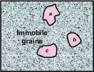
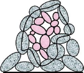
Figure 4: (a) Regions of mobile grains $a,b,c$ in a matrix of immobile grains below the Coulomb threshold. (b) Detail of pocket of mobile grains $a$ surrounded by immobile grains which are shaded.

The energy input must be on the level of noise, such that the grains largely remain in contact with one another, but are able to explore the energy landscape over a long period of time. In the case of external vibrations, the appropriate frequency and amplitude can be determined experimentally for different grain types, by investigating the motion of the individual grains or by monitoring the changes in the overall volume fraction over time. It is important that the amplitude does not exceed the gravitational force, or else the grains are free to fly up in the air, re-introducing the problem of initial creation just as they would if they were simply poured into another container.

Within a region $a$ we have a volume $\sum_{\alpha\in a}{\cal W}^{\alpha}$ and after the disturbance a volume which is now $\sum_{\alpha\in a}{\cal W}^{\prime\alpha}$ as seen in Fig. 3c. In Section 3.1 we have discussed how to define the volume function ${\cal W}^{\alpha}$ as a function of the contact network. Here the simplest “one grain” approximation is used as the “Hamiltonian” of the volume as defined by Eq. (6). In reality it is much more complicated, and although there is only one label $\alpha$ on the contribution of grain $\alpha$ to the volume, the characteristics of its neighbours may also appear. Instead of energy being conserved, it is the total volume which is conserved while the internal rearrangements take place within the pockets described above. Hence

$$\sum_{\alpha\in a}{{\cal W}^{\alpha}}=\sum_{\alpha\in a}{{\cal W}^{\prime\alpha}}$$ (19)

We now construct a Boltzmann equation. Suppose $z$ particles are in contact with grain $\alpha=0$, as seen in Fig. 3c. For rough particles $z=4$ while for smooth $z=6$ at the isostatic limit. The probability distribution will be of the contact points which are represented by the tensor ${\cal C}^{\alpha}$, Eq. (5), for each grain, where $\alpha$ ranges from 0 to 4 in this case. So the analogy of $f(v)$ for the Boltzmann gas equation becomes $f({\cal C}^{0})$ for the granular system and represents the probability that the external disturbance causes a particular motion of the grain. We therefore wish to derive an equation

$$\frac{\partial f({\cal C}^{0})}{\partial t}+\int{\cal K}({\cal C}^{\alpha},{\cal C}^{\prime\alpha})~{}~{}\Big{(}f_{0}f_{1}f_{2}f_{3}f_{4}-f^{\prime}_{0}f^{\prime}_{1}f^{\prime}_{2}f^{\prime}_{3}f^{\prime}_{4}\Big{)}~{}~{}d{\cal C}^{\prime 0}\prod_{\alpha\neq 0}d{\cal C}^{\alpha}d{\cal C}^{\prime\alpha}=0$$ (20)

The term $\cal K$ contains the condition that the volume is conserved (19), i.e. it must contain $\delta(\sum{\cal W}^{\alpha}-\sum{\cal W}^{\prime\alpha})$. The cross-section is now the compatibility of the changes in the contacts, i.e. ${\cal C}^{\alpha}$ must be replaced in a rearrangement by ${\cal C}^{\prime\alpha}$ (unless these grains part and make new contacts in which case a more complex analysis is called for). We therefore argue that the simplest $\cal K$ will depend on the external disturbance $\Gamma,\omega$ and on ${\cal C}^{\alpha}$ and ${\cal C}^{\prime\alpha}$, i.e.

$$\frac{\partial f({\cal C}^{0})}{\partial t}+\int\delta\Big{(}\sum_{\alpha}{\cal W}^{\alpha}-\sum_{\alpha}{\cal W}^{\prime\alpha}\Big{)}~{}{\cal J}({\cal C}^{\alpha},{\cal C}^{\prime\alpha})~{}~{}\Big{(}\prod_{\alpha=0}^{z}f_{\alpha}-\prod_{\alpha=0}^{z}f^{\prime}_{\alpha}\Big{)}d{\cal C}^{\prime 0}\prod_{\alpha\neq 0}d{\cal C}^{\alpha}d{\cal C}^{\prime\alpha}=0$$ (21)

where $\cal J$ is the cross-section and it is positive definite.

The Boltzmann argument now follows. As before

$$S=-\lambda\int f\log f\\ x=\frac{f_{0}f_{1}f_{2}f_{3}f_{4}}{f_{0}^{\prime}f_{1}^{\prime}f_{2}^{\prime}f_{3}^{\prime}f_{4}^{\prime}},$$ (22)

and

$$\frac{\partial S}{\partial t}\geq 0,$$ (23)

the equality sign being achieved when $x=1$ and

$$f_{\alpha}=\frac{e^{-{\cal W}^{\alpha}/\lambda X}}{Z},$$ (24)

with the partition function

$$Z=\sum e^{-{\cal W}^{\alpha}/\lambda X}~{}~{}~{}{\Theta},$$ (25)

and the analogue to the free energy being $Y=-X\ln Z$, and $X=\partial V/\partial S$.

The detailed description of the kernel $\cal K$ has not been derived as yet due to its complexity. Just as Boltzmann’s proof does not depend on the differential scattering cross section, only on the conservation of energy, in the granular problem we consider the steady state excitation externally which conserves volume, leading to the granular distribution function, Eq. (24).

It is interesting to note that there is a vast and successful literature of equilibrium statistical mechanics based on $\exp(-{\cal H}/k_{B}T)$, but a meagre literature on dynamics based on attempts to generalise the Boltzmann equation or, indeed, even to solve the Boltzmann equation in situations remote from equilibrium where it is still completely valid. It means that any advancement in understanding how it applies to analogous situations is a step forward.

5.1 Experimental Validation of the Statistical Mechanics Concepts

The first step in realising the idea of a general statistical jamming theory is to understand in detail the characteristics of a jammed configuration in particulate systems. Next we present a novel experimental method to explore this problem using confocal microscopy [12].

The key feature of this optical microscopy technique is that only light from the focal plane is detected. Thus 3D images of translucent samples can be acquired by moving the sample through the focal plane of the objective and acquiring a sequence of 2D images. Our model system consists of a dense packing of emulsion oil droplets, with a sufficiently elastic surfactant stabilising layer to mimic solid particle behaviour, suspended in a continuous phase fluid. The refractive index matching of the two phases, necessary for 3D imaging, is not a trivial task since it involves unfavourable additions to the water phase, disturbing surfactant activity. The successful emulsion system, stable to coalescence and Ostwald ripening, consisted of Silicone oil in a solution of water ($w_{t}=50\%$) and glycerol ($w_{t}=50\%$), stabilised by 0.01$mM$ sodium dodecylsulphate (SDS). The droplet phase is fluorescently dyed using Nile Red, prior to emulsification. The control of the particle size distribution, prior to imaging, is achieved by applying very high shear rates to the sample, inducing droplet break-up down to a radius mean size of $2\mu m$. Since the emulsion components have different densities, the droplets cream under gravity to form a random close packed structure. In addition, the absence of friction ensures that the system has no memory effects and reaches a true jammed state before measurement.

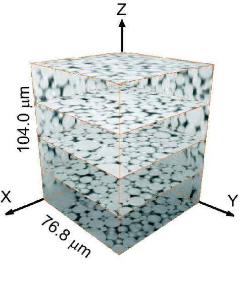
Figure 5: Confocal image of the densely packed emulsion system.

The 3D reconstruction of the 2D slices is shown in Fig. 5. We have developed a sophisticated image analysis algorithm which uses Fourier Filtering to determine the particle centres with subvoxel accuracy. Previously, we developed a method to measure the interdroplet forces and their distribution in the sample volume [12]. Using an extension to the same image analysis method, the 3D images of a densely packed particulate model system now allow for the characterisation of the volume function $\cal{W}$, by the partitioning of the images into first coordination shells of each particle, described in Section 3.1. The polyhedron obtained by such a partitioning is shown in Fig. 6.

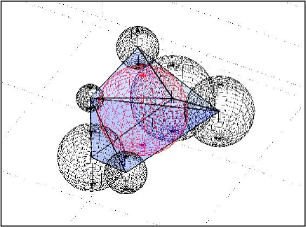
Figure 6: An example of a volume $\cal W$ as the polyhedron constructed from the 3D images. The centre grain (red) has 6 grains in contact (black), the centres of which are joined to form the polyhedron.

We are able to test how the approximation in Eq. (6) for the volume compares with the actual volume measured from the image for each grain. Their correlation is shown in Fig. 7. This approximation works well for coordination numbers larger than 3 in 2D and even in 3D, due to the partitioning of the obtained volumetric objects into triangles/pyramids, intrinsic to the method, and subsequently summing over them to obtain the resulting volume. It is clear that very large volumes, belonging to grains with high coordination numbers, do stray from the theoretical value due to the complex geometries involved. According to the experimental measurements of $\cal{W}$ employed in this study, the total volume of the system was found to be overestimated by only $\approx 5\%$.

Figure 7: $\cal W$ function obtained from the configuration tensor $\cal C$ are plotted against the polyhedra constructed from the images.

The ability to measure this function and therefore its fluctuations in a given particle ensemble, enables the calculations of the macroscopic variables. In Fig. 8 we show the probability distribution of ${\cal W}$ showing an exponential behaviour as given by Eq. (24). The exponential probability distribution of $\cal{W}$ leads to the compactivity $X$ according to Eq. (18). This implies that we can arrive at the thermodynamic system properties from the knowledge of the microstructure. Many images, i.e. configurations, can be treated in this way to test whether system size influences the macroscopic observables. If the particles are subjected to ultracentrifugation resulting in configurations of a higher density, the influence of pressure on the macroscopic variables can also be tested.

Figure 8: Probability distribution of $\cal W$ fitted with a single exponential. The decay constant is the compactivity, $X=119\mu m^{3}/\lambda$.

Such a characterisation of the governing macroscopic variables, arising from the information of the microstructure, allows one to predict the system’s behaviour through an equation of state. This is the first experimental study of such statistical concepts in particulate matter and opens new possibilities for testing the above described thermodynamic formulation. In principle, one can apply low amplitude vibrations to the system and observe the droplet configuration before and after the perturbation, thus testing the ideas proposed in the Boltzmann derivation.

Acknowledgments. We thank D. Grinev and R. Blumenfeld for stimulating discussions. H. Makse acknowledges financial support from the National Science Foundation, DMR-0239504 and the Department of Energy, Division of Materials Sciences and Engineering, DE-FE02-03ER46089.

References

- [1] E. R. Nowak, J. B. Knight, E. BenNaim, H. M. Jaeger and S. R. Nagel. Phys. Rev. E 57, 1971 (1998).
- [2] S. F. Edwards and R. B. S. Oakeshott, Physica A 157, 1080-1090 (1989).
- [3] S. F. Edwards, in Granular matter: an interdisciplinary approach (ed. A. Mehta) 121-140 (Springer-Verlag, New York, 1994).
- [4] H. A. Makse, J. Brujić, and S. F. Edwards, in The Physics of Granular Media, (eds. H. Hinrichsen and D. E. Wolf) (Wiley-VCH, 2004).
- [5] R. C. Ball and R. Blumenfeld, Phys. Rev. Lett. 88, 115505 (2002).
- [6] P. Philippe, and D. Bideau, Europhys. Lett. 60, 677 (2002).
- [7] J. Brujić, D. L. Johnson, O. Sindt, and H. A. Makse (Schlumberger report, to be published).
- [8] A. Chakravarty, S. F. Edwards, D. V. Grinev, M. Mann, T. E. Phillipson, A. J. Walton, Proceedings of the Workshop on Quasi-static Deformations of Particulate Materials, to be published.
- [9] H. A. Makse and J. Kurchan, Nature 415, 614-617 (2002).
- [10] S. B. Savage, Adv. Appl. Mech. 24, 289-365 (1994).
- [11] J. T. Jenkins, and S. B. Savage, J. Fluid Mech. 130, 187-202 (1983).
- [12] J. Brujić, S. F. Edwards, I. Hopkinson, and H. A. Makse, Physica A 327, 201-212 (2003).