Doping dependence of the electron-doped cuprate superconductors from the antiferromagnetic properties of the Hubbard model

Abstract

Within the Kotliar-Ruckenstein slave-boson approach, we have studied the antiferromagnetic (AF) properties for the $t$-$t^{\prime}$-$t^{\prime\prime}$-$U$ model applied to electron-doped cuprate superconductors. It is found that, due to the inclusion of quantum fluctuations, the AF order decays with increasing doping much faster than obtained in the Hartree-Fock theory. Under an intermediate constant $U$ the calculated doping evolution of the spectral intensity in the AF state has satisfactorily reproduced the experimental results, without need of a strongly doping-dependent $U$ as argued earlier. This may reconcile a discrepancy in recent studies on photoemission and optical conductivity.

I Introduction

The intriguing Fermi surface (FS) evolution with doping in electron-doped cuprate Nd_2-xCe_xCuO₄ revealed by angle-resolved photoemission spectroscopy (ARPES) measurementsArmitage ; Matsui has attracted much attention recently.Kusko ; Markiewicz ; Kyung ; Senechal ; Kusunose ; Lee ; Yuan04 ; Yuan05 ; Tohyama ; Luo It was observed that at low doping a small FS pocket appears around $(\pi,0)$. Upon increased doping a new pocket begins to emerge around $(\pi/2,\pi/2)$ and eventually at optimal doping $x=0.15$ the several FS pieces connect to form a large curve around $(\pi,\pi)$. By use of the $t$-$t^{\prime}$-$t^{\prime\prime}$-$U$ model and Hartree-Fock (HF) mean-field treatment, Kusko et al.Kusko have studied the FS in consideration of the antiferromagnetic (AF) order and reached remarkable agreement with experiments. However, in their work the on-site $U$ is treated as a doping-dependent effective parameter, specifically $U=6t$ at doping $x=0$ and $3.1t$ at $x=0.15$. Similarly a doping-dependent $U$ was argued by others based on numerical calculations.Kyung ; Senechal Alternatively, the strong-coupling $t$-$t^{\prime}$-$t^{\prime\prime}$-$J$ model was adopted by some of us to construct the FS.Yuan04 Without tuning parameters we have also obtained consistent results with ARPES data.

Very recently, a systematic analysis of the optical conductivity for electron-doped cuprates was undertaken by Millis et al.Millis It suggests that (i) the electron-doped materials are approximately as strongly correlated as the hole-doped ones and (ii) the $U$ value is not strongly doping dependent within the electron-doped family. Both of these implications are in apparent disagreement with the theoretical studies by Kusko et al.,Kusko and in favor of the strong-coupling model used by us.Yuan04 On the other hand, our result at optimal doping from the $t$-$t^{\prime}$-$t^{\prime\prime}$-$J$ modelYuan04 has not been reconciled by exact diagonalization calculations.Tohyama Thus it is still open whether the strong-coupling model, as implied by point (i) above, is available to explain the ARPES data at optimal doping.

Here our attention is focused on the issue relevant to point (ii) above, i.e., for the $t$-$t^{\prime}$-$t^{\prime\prime}$-$U$ model whether the strong doping dependence of $U$ as argued by Kusko et al.Kusko ; Markiewicz is really necessary for the interpretation of ARPES data. Theoretically it is not convincing to have a strongly doping-dependent $U$ since it is a local interaction within an atom and difficult to be changed by adding carriers. To understand why a strongly doping-dependent $U$ is needed by Kusko et al., we come to some details of their work. Within the HF mean-field theory, two AF energy bands are derived, with the minimum of the upper band around $(\pi,0)$ and the maximum of the lower one around $(\pi/2,\pi/2)$. At low electron-doping, the upper band is crossed by the Fermi level, leading to a small FS pocket around $(\pi,0)$. With increasing doping, the AF order weakens and the lower band shifts towards the Fermi level. The essential observation is that the AF order decays with doping too slowly under a constant $U$, and consequently the lower band is still too far away from the Fermi level even at optimal doping to contribute any spectral intensity around $(\pi/2,\pi/2)$. Therefore an effective $U(x)$, which decreases with increasing $x$, is enforced to expedite the decline of the AF order so that the lower band approaches the Fermi level rapidly leading to the consistency with ARPES results.

Actually, as we know, the HF theory overestimates the AF order due to the ignorance of fluctuations. So a tempting idea is that the real AF order should decay with doping in a (much) quicker way than obtained in the HF theory. Then it is interesting to ask how much the HF results will be improved if the fluctuations are taken into account and whether the ARPES data can already be explained with a doping-independent $U$. In this paper we try to answer these questions by studying the $t$-$t^{\prime}$-$t^{\prime\prime}$-$U$ model with the Kotliar-Ruckenstein slave-boson (SB) approach.KR The method well considers the AF fluctuations for a wide range of interactionsLilly ; Yuan02 and has been used to study the stripes in hole-doped cuprates.Seibold We have found that, compared to the HF results, the AF state derived from the SB approach has a much lower energy and the order parameter decreases much faster with doping. Consequently, the ARPES results can be reproduced under a constant $U$.

II Formalism

We start with the $t$-$t^{\prime}$-$t^{\prime\prime}$-$U$ model on a square lattice which reads

$$H = -t\sum_{\langle ij\rangle\sigma}(c_{i\sigma}^{\dagger}c_{j\sigma}+{\rm h.c.})-t^{\prime}\sum_{\langle ij\rangle_{2}\sigma}(c_{i\sigma}^{\dagger}c_{j\sigma}+{\rm h.c.})$$ (1)

$$-t^{\prime\prime}\sum_{\langle ij\rangle_{3}\sigma}(c_{i\sigma}^{\dagger}c_{j\sigma}+{\rm h.c.})+U\sum_{i}n_{i\uparrow}n_{i\downarrow}\ ,$$

where $\langle\rangle,\ \langle\rangle_{2},\ \langle\rangle_{3}$ represent the nearest neighbor (n.n.), second n.n., and third n.n. sites, respectively, and the rest of the notation is standard. Throughout the work $t$ is taken as the energy unit and typical parameters $t^{\prime}=-0.3$ and $t^{\prime\prime}=0.2$ are adopted.

In the spirit of the Kotliar-Ruckenstein SB approach,KR four auxiliary bosons $e_{i}^{(\dagger)},\ p_{i\sigma}^{(\dagger)}\ (\sigma=\uparrow,\downarrow),\ d_{i}^{(\dagger)}$ are introduced at each site to label the four different states, which can be empty, singly occupied by an electron with spin up or down, or doubly occupied. The advantage of introducing bosons is that the interaction term can be linearized, i.e., the product of density operators $n_{i\uparrow}n_{i\downarrow}$ is replaced by $d_{i}^{\dagger}d_{i}$, the occupation number operator for double occupancy. As the expense, the hopping term becomes complicated because any hopping process of electrons must be accompanied by the transitions of slave bosons. Explicitly, if an electron (with spin $\sigma$) hops from site $i$ to $j$, the slave bosons must change simultaneously at both sites $i$ and $j$. For example, at site $i$, associated with the annihilation of the electron the bosonic state will transit either from the singly occupied one with spin $\sigma$ to the empty one or from the doubly occupied one to the singly occupied one with spin $\bar{\sigma}$. Namely, the transition of the bosons at site $i$ can be described by the operator $z_{i\sigma}=e_{i}^{\dagger}p_{i\sigma}+p_{i\bar{\sigma}}^{\dagger}d_{i}$. To eliminate the unphysical states in the enlarged (fermionic and bosonic) Hilbert space, the following constraints have to be imposed at each site:

$$e_{i}^{\dagger}e_{i}+\sum_{\sigma}p_{i\sigma}^{\dagger}p_{i\sigma}+d_{i}^{\dagger}d_{i} = 1\ ,$$ (2)

$$p_{i\sigma}^{\dagger}p_{i\sigma}+d_{i}^{\dagger}d_{i} = c_{i\sigma}^{\dagger}c_{i\sigma}\ .$$ (3)

The first constraint states that a site is either empty, singly occupied, or doubly occupied. And the second one guarantees that, when an electron with spin $\sigma$ locates at site $i$, this site is either singly occupied with spin $\sigma$ or doubly occupied.

In order to study the AF order, we divide the lattice into two sublattices $A$ and $B$. For sublattice $L$ ($L=A,B$), we introduce a set of bosons $e_{iL}^{(\dagger)},\ p_{iL\sigma}^{(\dagger)}\ (\sigma=\uparrow,\downarrow),\ d_{iL}^{(\dagger)}$, and Lagrange multipliers $\lambda_{iL}^{1},\ \lambda_{iL}^{\sigma}$ which are associated with the constraints (2) and (3), respectively. Thus the original Hamiltonian, with Lagrange multiplier terms added, can be rewritten, in terms of fermionic operators $a$ and $b$ corresponding to sublattice $A$ and $B$ respectively, as follows

$$H = -t\sum_{\langle ij\rangle\sigma,i\in A}(z_{iA\sigma}^{\dagger}a_{i\sigma}^{\dagger}b_{j\sigma}z_{jB\sigma}+{\rm h.c.})-t\sum_{\langle ij\rangle\sigma,i\in B}(z_{iB\sigma}^{\dagger}b_{i\sigma}^{\dagger}a_{j\sigma}z_{jA\sigma}+{\rm h.c.})-t^{\prime}\sum_{\langle ij\rangle_{2}\sigma,i\in A}(z_{iA\sigma}^{\dagger}a_{i\sigma}^{\dagger}a_{j\sigma}z_{jA\sigma}+{\rm h.c.})$$ (4)

$$-t^{\prime}\sum_{\langle ij\rangle_{2}\sigma,i\in B}(z_{iB\sigma}^{\dagger}b_{i\sigma}^{\dagger}b_{j\sigma}z_{jB\sigma}+{\rm h.c.})-t^{\prime\prime}\sum_{\langle ij\rangle_{3}\sigma,i\in A}(z_{iA\sigma}^{\dagger}a_{i\sigma}^{\dagger}a_{j\sigma}z_{jA\sigma}+{\rm h.c.})-t^{\prime\prime}\sum_{\langle ij\rangle_{3}\sigma,i\in B}(z_{iB\sigma}^{\dagger}b_{i\sigma}^{\dagger}b_{j\sigma}z_{jB\sigma}+{\rm h.c.})$$

$$+U\sum_{i\in A}d_{iA}^{\dagger}d_{iA}+U\sum_{i\in B}d_{iB}^{\dagger}d_{iB}+\sum_{i\in A}\lambda_{iA}^{1}(1-e_{iA}^{\dagger}e_{iA}-\sum_{\sigma}p_{iA\sigma}^{\dagger}p_{iA\sigma}-d_{iA}^{\dagger}d_{iA})+\sum_{i\in A,\sigma}\lambda_{iA}^{\sigma}(a_{i\sigma}^{\dagger}a_{i\sigma}-p_{iA\sigma}^{\dagger}p_{iA\sigma}-d_{iA}^{\dagger}d_{iA})$$

$$+\sum_{i\in B}\lambda_{iB}^{1}(1-e_{iB}^{\dagger}e_{iB}-\sum_{\sigma}p_{iB\sigma}^{\dagger}p_{iB\sigma}-d_{iB}^{\dagger}d_{iB})+\sum_{i\in B,\sigma}\lambda_{iB}^{\sigma}(b_{i\sigma}^{\dagger}b_{i\sigma}-p_{iB\sigma}^{\dagger}p_{iB\sigma}-d_{iB}^{\dagger}d_{iB})\ ,$$

where the operators

$$z_{iL\sigma}={e_{iL}^{\dagger}p_{iL\sigma}+p_{iL\bar{\sigma}}^{\dagger}d_{iL}\over\sqrt{(1-e_{iL}^{\dagger}e_{iL}-p_{iL\bar{\sigma}}^{\dagger}p_{iL\bar{\sigma}})(1-d_{iL}^{\dagger}d_{iL}-p_{iL\sigma}^{\dagger}p_{iL\sigma})}}$$

have been renormalizedKR to ensure the exact result at $U=0$ even in mean-field treatment as adopted subsequently. With mean-field approximation, the bosons are replaced by c numbers and assumed to be site-independent on each sublattice, i.e., $\langle e_{iL}^{(\dagger)}\rangle=e_{L},\ \langle p_{iL\sigma}^{(\dagger)}\rangle=p_{L\sigma},\ \langle d_{iL}^{(\dagger)}\rangle=d_{L}$ (and correspondingly $\langle z_{iL\sigma}^{(\dagger)}\rangle=z_{L\sigma}$). At the same time, the constraints are softened to be satisfied only on the average on each sublattice, i.e., $\lambda_{iL}^{1}\rightarrow\lambda_{L}^{1},\ \lambda_{iL}^{\sigma}\rightarrow\lambda_{L}^{\sigma}$. This treatment is equivalent to making a saddle-point approximation in the path-integral formulation. Now the Hamiltonian becomes quadratic in terms of fermionic operators and can be easily diagonalized in momentum space. Finally we have

$$H = \sum_{k\sigma}(E_{k\sigma}^{-}\tilde{a}_{k\sigma}^{\dagger}\tilde{a}_{k\sigma}+E_{k\sigma}^{+}\tilde{b}_{k\sigma}^{\dagger}\tilde{b}_{k\sigma})+E_{0}\ ,$$ (5)

where the energy bands read

$$E_{k\sigma}^{\pm}=[\lambda_{A}^{\sigma}+\lambda_{B}^{\sigma}+(z_{A\sigma}^{2}+z_{B\sigma}^{2})\varepsilon^{\prime}_{k}]/2\pm\sqrt{[\lambda_{B}^{\sigma}-\lambda_{A}^{\sigma}+(z_{B\sigma}^{2}-z_{A\sigma}^{2})\varepsilon^{\prime}_{k}]^{2}/4+(z_{A\sigma}z_{B\sigma}\varepsilon_{k})^{2}}$$ (6)

with

$$\varepsilon_{k} = -2t(\cos k_{x}+\cos k_{y})\ ,$$

$$\varepsilon^{\prime}_{k} = -4t^{\prime}\cos k_{x}\cos k_{y}-2t^{\prime\prime}(\cos 2k_{x}+\cos 2k_{y})\ ,$$

and the constant

$$E_{0} = (N/2)\left[U(d_{A}^{2}+d_{B}^{2})-\lambda_{A}^{1}(e_{A}^{2}+\sum_{\sigma}p_{A\sigma}^{2}+d_{A}^{2}-1)\right.$$

$$\ \ \ \ \ \ \ \ \ \ -\lambda_{B}^{1}(e_{B}^{2}+\sum_{\sigma}p_{B\sigma}^{2}+d_{B}^{2}-1)$$

$$\ \ \ \ \ \ \ \ \ \ \left.-\sum_{\sigma}\lambda_{A}^{\sigma}(p_{A\sigma}^{2}+d_{A}^{2})-\sum_{\sigma}\lambda_{B}^{\sigma}(p_{B\sigma}^{2}+d_{B}^{2})\right]\ .$$

Above $N$ is the total number of lattice sites, $k$ is restricted to the magnetic Brillouin zone (BZ), and the operators $\tilde{a}$ and $\tilde{b}$ are related to $a$ and $b$ by unitary transformations.

The grand canonical thermodynamic potential is given by [$\beta=1/(k_{B}T)$ with $T$: temperature]

$$\Omega=-{1\over\beta}\sum_{k\sigma}\sum_{\nu=+,-}\ln\left[1+e^{-\beta(E_{k\sigma}^{\nu}-\mu)}\right]+E_{0}\ .$$ (7)

Here $\mu$ is the chemical potential decided by $-(\partial\Omega/\partial\mu)=N_{e}$ ($N_{e}$ is the total number of electrons). All the parameters are determined to give the lowest free energy $F=\Omega+N_{e}\mu$. The calculation will be simplified if we search for the AF solution which satisfies the relations: $e_{A}=e_{B},\ d_{A}=d_{B},\ p_{A\sigma}=p_{B\bar{\sigma}},\ \lambda_{A}^{1}=\lambda_{B}^{1},\ \lambda_{A}^{\sigma}=\lambda_{B}^{\bar{\sigma}}$. (Correspondingly the energy bands $E_{k\sigma}^{\pm}$ become spin degenerate, i.e., $E_{k\sigma}^{\pm}=E_{k}^{\pm}$.) The staggered magnetization, which characterizes the AF order, is given by $m=(p_{A\uparrow}^{2}-p_{A\downarrow}^{2})/2=(p_{B\downarrow}^{2}-p_{B\uparrow}^{2})/2$.

III Results

In the following we are limited to $T=0$ only at which the AF long-range order is possible for the two-dimensional model.

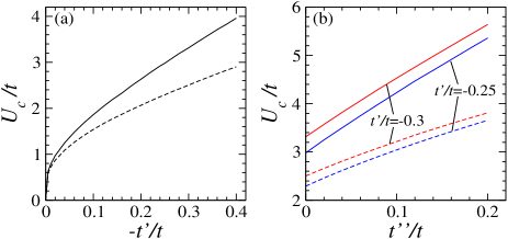
Figure 1: (Color online) The critical $U_{c}$ for the AF order to be stabilized at half filling: (a) $U_{c}$ vs $-t^{\prime}$ when $t^{\prime\prime}=0$ (b) $U_{c}$ vs $t^{\prime\prime}$ at fixed $t^{\prime}/t=-0.25$ [blue (black) lines] and $-0.3$ [red (dark gray) lines]. All solid lines are from SB approach and dashed ones from HF theory.

To look at the differences between SB and HF results, we first consider the half-filled case, i.e., $n=N_{e}/N=1$. As is well known, the pure $t$-$U$ (with $t^{\prime}=t^{\prime\prime}=0$) model takes on the AF order for arbitrarily small $U>0$ due to the perfect nesting effect. After inclusion of the long-range hoppings, the AF order will be frustrated and a critical $U=U_{c}$ is required to stabilize it. The relations between $U_{c}$ and $t^{\prime}$, $t^{\prime\prime}$ from both SB and HF approaches are compared in Fig. 1. While Fig. 1(a) shows $U_{c}$ vs $t^{\prime}$ when $t^{\prime\prime}=0$ which has been given previously,Trapper we further present $U_{c}$ vs $t^{\prime\prime}$ at fixed $t^{\prime}$ in Fig. 1(b). It is clear that $U_{c}$ increases with both $t^{\prime}$ and $t^{\prime\prime}$. Moreover, the value of $U_{c}$ at fixed $t^{\prime}$ and $t^{\prime\prime}$ obtained from SB approach is always larger than that from HF theory. This is expected in view that the HF theory overestimates the AF order. Once the fluctuations are taken into account, the critical value $U_{c}$ will be largely raised as seen in the SB approach. We notice that for parameters $t^{\prime}=-0.25$ and $t^{\prime\prime}=0.1$ as adopted by Kusko et al.Kusko the accurate critical value is $U_{c}=4.23$ from SB approach rather than $3.05$ from HF theory. Thus those values for doping-dependent $U$ selected by them,Kusko i.e., $U=3.5(3.1)$ at $x=0.1(0.15)$ are actually unreasonable, which are already too small to stabilize the AF order.

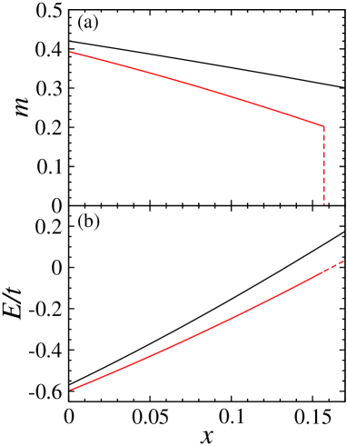
Figure 2: (Color online) Staggered magnetization (a) and ground state energy (b) vs electron doping for parameters $t^{\prime}=-0.3$, $t^{\prime\prime}=0.2$ and $U=6.3$. The red (dark gray) lines are from SB approach and black ones from HF theory. The dashed line in panel (a) shows that $m$ jumps to zero at $x\simeq 0.157$ in SB approach, and correspondingly the dashed one in panel (b) gives the energy at $m=0$.

Then we come to see how the AF order declines with increasing doping $x(=n-1)$ under fixed $U$. For $t^{\prime}=-0.3$ and $t^{\prime\prime}=0.2$, the critical value at half filling is $U_{c}=5.64$(SB)$/3.81$(HF). We choose $U=6.3>U_{c}$ and solve the self-consistent equations. The staggered magnetization $m$ as a function of $x$ is shown in Fig. 2(a), where the red (dark gray) and black lines are obtained from SB and HF approaches, respectively. It is seen that at half filling the AF order derived from SB approach becomes weak relative to that from HF theory. And it is even weaker with increasing doping because $m$ decreases much faster in SB approach than in HF theory. In addition, we have found that the AF state becomes energetically unfavorable at $x\simeq 0.157$ in SB approach, leading to a first-order transition as shown by the dashed line in Fig. 2(a). This first-order termination of the AF order, compared to the claim of a quantum critical point,Kyung seems to be closer to the experimental observation where a steep disappearance of the AF phase was found.Fujita Also the doping range that the AF order survives is quantitatively consistent with experiment.Mang In contrast, $m$ keeps finite up to $x\sim 0.4$ and goes to zero continuously in HF theory (not shown). The corresponding ground state energies from both approaches are compared in Fig. 2(b). The energy derived from SB approach is notably lower than that from HF theory and the energy difference increases with increasing doping. This indicates that the study of the AF property is largely improved within the SB approach.

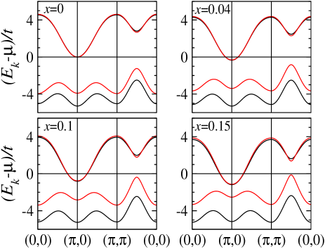
Figure 3: (Color online) The energy bands at different dopings. In each panel, the red (dark gray) and black lines are from SB and HF approaches, respectively. The Fermi energy is fixed at zero.

Subsequently the energy bands $E_{k}^{\pm}-\mu$ are plotted in Fig. 3, with red (dark gray) lines from SB approach and black ones from HF theory. (The definitions of $E_{k}^{\pm}$ in the magnetic BZ have been analytically extended to the original BZ.) While the upper bands derived from two approaches look similar at each doping, the lower bands take on different behaviors. Within HF theory, the lower band shifts very slowly towards the Fermi level with increasing doping and is still far away from it at $x=0.15$. On the other hand, within SB approach, the lower band lifts towards the Fermi level as a whole. At $x=0.1$ it is already rather close to the latter and may contribute the spectral intensity within the experimental resolution. At optimal doping, it is nearly crossed by the Fermi level around $(\pi/2,\pi/2)$.

In order to directly compare with the ARPES data, we have calculated the spectral function $A(k,\omega)$ within SB approach. The density plots for integration of $A(k,\omega)$ times the Fermi function over an energy interval $[-40,20]$ meV (same as that adopted in ARPES experimentsArmitage ) around the Fermi level are shown in Fig. 4 by the top row. At low doping $x=0.04$ a small FS pocket forms around $(\pi,0)$ [and equivalently $(0,\pi)$]. At doping $x=0.1$ the spectral intensity begins to appear around $(\pi/2,\pi/2)$, and becomes strong at optimal doping. At the same time, the Fermi patch around $(\pi,0)$ deforms with increasing doping, i.e., half of the FS around $(\pi,0)$ loses much of its intensity. The theoretical results agree well with the ARPES data.Armitage For comparison, the corresponding plots from HF theory are shown by the bottom row in Fig. 4, which, however, do not exhibit the main experimental features.

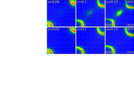
Figure 4: (Color online) Density plots for integration of $A(k,\omega)$ times the Fermi function over an energy interval $[-0.12,0.06]t\simeq[-40,20]$ meV around the Fermi level, at doping $x=0.04$, $0.1$ and $0.15$ (from left to right). The top row is from the SB approach and the bottom row from HF theory, under a doping-independent constant $U=6.3$ (with $t^{\prime}=-0.3$ and $t^{\prime\prime}=0.2$). The Lorentzian broadening is $0.15t$.

IV Discussions and Conclusion

In the above sections, after suitable consideration of the AF fluctuations we have reached consistent results with ARPES measurements under a doping-independent constant $U$, in contrast with the previous argument for a doping-dependent $U$.Kusko ; Markiewicz ; Kyung ; Senechal The agreement is satisfactory in view that all input parameters except $U$ are extracted from experiments. We do not exclude that a tunable $U$ with doping will help lead to a perfect comparison between theory and experiment. Even in this case, however, not a strong doping-dependence of $U$ as given by Kusko et al. ($\sim 50$% variation from $x=0$ to $x=0.15$)Kusko is needed. This may reconcile one of the discrepancies in recent explanations of both ARPES and optical conductivity mentioned before.

As for the magnitude of $U$, an intermediate value $6.3t$ is adopted here, which is somewhat too small at $x=0$ to produce the observed Mott gap ($\sim 1$ eV)Armitage in the parent compounds of electron-doped cuprates. A larger $U\sim 8t$ is expected, but it will be unfavorable to the appearance of the spectral intensity around $(\pi/2,\pi/2)$ in our current calculation. On the other hand, we should note that, if the AF fluctuations are fully taken into account, an even quicker decreasing of $m$ with doping than displayed in Fig. 2(a) will be the case. Then a larger $U$ than adopted here, towards strong-coupling regime, could be chosen and fixed throughout the doping range, leading to the similar intensity maps shown in the top row of Fig. 4. The evaluation of the biggest $U$ available to explain the ARPES data as well as the possibility to cross over to the strong-coupling model need further work.Dahnken

In conclusion, we have studied the AF properties for the electron-doped $t$-$t^{\prime}$-$t^{\prime\prime}$-$U$ model by use of the Kotliar-Ruckenstein SB approach. With inclusion of quantum fluctuations the AF order declines with increasing doping much faster than obtained in the HF theory. The calculated doping evolution of the spectral intensity under a constant $U$ is in good agreement with ARPES measurements on electron-doped cuprates. A strongly doping-dependent $U$, which is difficult to justify itself, is found to be actually unnecessary.

References

- (1) N. P. Armitage, F. Ronning, D. H. Lu, C. Kim, A. Damascelli, K. M. Shen, D. L. Feng, H. Eisaki, Z.-X. Shen, P. K. Mang, N. Kaneko, M. Greven, Y. Onose, Y. Taguchi, and Y. Tokura, Phys. Rev. Lett. 88, 257001 (2002).
- (2) H. Matsui, K. Terashima, T. Sato, T. Takahashi, S.-C. Wang, H.-B. Yang, H. Ding, T. Uefuji, and K. Yamada, Phys. Rev. Lett. 94, 047005 (2005).
- (3) C. Kusko, R. S. Markiewicz, M. Lindroos, and A. Bansil, Phys. Rev. B 66, 140513(R) (2002).
- (4) R. S. Markiewicz, Phys. Rev. B 70, 174518 (2004).
- (5) B. Kyung, V. Hankevych, A.-M. Daré, and A.-M. S. Tremblay, Phys. Rev. Lett. 93, 147004 (2004).
- (6) D. Sénéchal and A.-M. S. Tremblay, Phys. Rev. Lett. 92, 126401 (2004).
- (7) H. Kusunose and T. M. Rice, Phys. Rev. Lett. 91, 186407 (2003).
- (8) T. K. Lee, C. M. Ho, and N. Nagaosa, Phys. Rev. Lett. 90, 067001 (2003).
- (9) Q. S. Yuan, Y. Chen, T. K. Lee, and C. S. Ting, Phys. Rev. B 69, 214523 (2004).
- (10) Q. S. Yuan, T. K. Lee, and C. S. Ting, Phys. Rev. B 71, 134522 (2005).
- (11) T. Tohyama, Phys. Rev. B 70, 174517 (2004).
- (12) H. G. Luo and T. Xiang, Phys. Rev. Lett. 94, 027001 (2005).
- (13) A. J. Millis, A. Zimmers, R. P. S. M. Lobo, and N. Bontemps, cond-mat/0411172.
- (14) G. Kotliar and A. E. Ruckenstein, Phys. Rev. Lett. 57, 1362 (1986).
- (15) L. Lilly, A. Muramatsu, and W. Hanke, Phys. Rev. Lett. 65, 1379 (1990).
- (16) Q. S. Yuan and T. Kopp, Phys. Rev. B 65, 085102 (2002).
- (17) G. Seibold and J. Lorenzana, Phys. Rev. B 69, 134513 (2004).
- (18) U. Trapper, H. Fehske, and D. Ihle, Physica C 282-287, 1779 (1997); I. Yang, E. Lange, and G. Kotliar, Phys. Rev. B 61, 2521 (2000).
- (19) M. Fujita, T. Kubo, S. Kuroshima, T. Uefuji, K. Kawashima, K. Yamada, I. Watanabe, and K. Nagamine, Phys. Rev. B 67, 014514 (2003).
- (20) P. K. Mang, O. P. Vajk, A. Arvanitaki, J. W. Lynn, and M. Greven, Phys. Rev. Lett. 93, 027002 (2004).
- (21) This possibility seems to be supported from the very recent numerical study, see C. Dahnken, M. Potthoff, E. Arrigoni, and W. Hanke, cond-mat/0504618.