The number of link and cluster states: the core of the 2D $q$ state Potts model

Abstract

Due to Fortuin and Kastelyin the $q$ state Potts model has a representation as a sum over random graphs, generalizing the Potts model to arbitrary $q$ is based on this representation. A key element of the Random Cluster representation is the combinatorial factor $\Gamma_{\mathcal{G}}(\mathsf{C_{\mathcal{}}},\mathsf{E_{\mathcal{}}})$, which is the number of ways to form $\mathsf{C_{\mathcal{}}}$ distinct clusters, consisting of totally $\mathsf{E_{\mathcal{}}}$ edges. We have devised a method to calculate $\Gamma_{\mathcal{G}}(\mathsf{C_{\mathcal{}}},\mathsf{E_{\mathcal{}}})$ from Monte Carlo simulations.

1 Introduction

The Potts model[1] is one of the most studied models in statistical physics. The traditional representation of the model is in terms of the Hamiltonian

$$H=-J\sum_{\langle i,j\rangle}\delta(\sigma_{i},\sigma_{j}),$$ (1)

where the spins $\sigma_{i}$ are integer values $\sigma_{i}\in[1\ldots q]$, the sum $\langle i,j\rangle$ is over nearest neighbours. The $q$ is a parameter of the model. The model is typically defined on a regular lattice in $d$ dimensions, but can in general be defined on any graph.

For $d\geq 2$ the model sustains a order-disorder transition , in $d=2$ the critical coupling is $\beta_{c}=\ln(1+\sqrt{q})$. For $\beta>\beta_{c}$ the $q$-fold permutation symmetry of Eq. 1 is broken, and one of the $q$ different groundstates has been singled out. For $q=2$ the model is the familiar Ising model, which has a second order transition, but with increasing $q$ the excited states have relatively more entropy and for $q>q_{c}$ the transition is first order. For $d=2$ the phase transition changes order at $q_{c}=4$ [2, 3], for $d=3$ the exact value is not known, but the most recent estimate based on Monte Carlo simulations is $q_{c}\approx 2.35$[4].

The Hamiltonian Eq. 1 is only defined for integer $q$, however due to an elegant transformation by Fortuin and Kastelyn (KF) the partition function of the $q$ state Potts model can be written as a correlated percolation problem, the socalled Random Cluster (RC) model[5]. In the RC representation $q$ enters as an ordinary variable, and can attain any scalar value. Apart from extrapolation/interpolation from integer $q$ results, all (numerical) studies of the noninteger $q$ properties of the Potts model are based on the RC representation, this also applies to the current paper. Properties of the Potts model with noninteger $q$ have been extensively studied using transfer matrix[6] techniques. Recently also MC simulations have been used. The latter come in two categories; either a technique is based on the RC measure to simulate directly at an arbitrary $q$[4, 7, 8], or alternatively the results are reweighted to arbitrary $q$ after the simulation is complete[7, 9].

The rest of this paper is organized as follows: In section 2 we introduce some key elements of graph theory, and how concepts from graph theory can be applied in statistical physics; in particular to the Potts model. In section 3 we introduce and describe an algorithm which can be used to “reweight” Potts model simulations to arbitrary $q$. Section 4 is devoted to results, both to show the correctness of the approach and also to study real $q$ properties which are not easily studied by ordinary MC simulations.

2 Graph theory and the Potts model

An (undirected) graph $\mathcal{G}$ is a collection of vertices $V(\mathcal{G})$, along with a set of edges $E(\mathcal{G})$ connecting the vertices[10]. A subgraph $\mathcal{G^{\prime}}\in\mathcal{G}$ is a collection of vertices and edges such that $V(\mathcal{G^{\prime}})\in V(\mathcal{G})$ and $E(\mathcal{G^{\prime}})\in E(\mathcal{G})$. The rank of a graph is denoted by $r(\mathcal{G})$ and given by

$$r(\mathcal{G})=\left|V(\mathcal{G})\right|-C(\mathcal{G}),$$ (2)

where $\left|V(\mathcal{G})\right|$ is the number of vertices and $C(\mathcal{G})$ is the number of connected components. Observe that also isolated single vertices constitute connected components when evaluating the rank of a graph. Fig. 1 shows a simple graph and illustrates the necessary concepts. From now on we will use the symbols $\mathsf{E_{\mathcal{G}}}$, $\mathsf{C_{\mathcal{G}}}$ and $\mathsf{V_{\mathcal{G}}}$ to denote the number of edges, clusters and vertices in a graph $\mathcal{G}$, when there is no ambiguity we will omit the index $\mathcal{G}$.

Figure 1: The sites of $5\times 5$ lattice, and links connecting some of the sites. Together these sites and links constitute a graph. This particular graph has $\mathsf{V_{\mathcal{G}}}=25$, $\mathsf{E_{\mathcal{G}}}=20$, six connected components ($\mathsf{C_{\mathcal{G}}}=6$) and a rank $r(\mathcal{G})=\mathsf{V_{\mathcal{G}}}-\mathsf{C_{\mathcal{G}}}=19$.

By assigning scalar properties to sites and bonds one can define different graph polynomials. One of the most general graph polynomials is the Tutte or Di-Chromatic polynomal $T_{\mathcal{G}}(x,y)$[11, 12]:

$$T_{\mathcal{G}}(x,y)=\sum_{E\in E(\mathcal{G})}\left(x-1\right)^{r(E)-r(\mathcal{\mathcal{G}})}\left(y-1\right)^{\mathsf{E_{\mathcal{}}}-r(\mathcal{G})}.$$ (3)

The sum in Eq. 3 is over all edge configurations of the graph $\mathcal{G}$ (i.e. spanning subgraphs). Here $x$ is a scalar property assigned to the vertex set, and $y$ a property assigned to the edges; as indicated in Eq. 3 we will only consider the situation of spatially constant $y$, but the general definition of the Tutte polynomial allows for a set $\left\{y\right\}$ of edge properties. Many other polynomials can be found as suitably rescaled evaluations of the Tutte polynomial[13]:

$$R_{\mathcal{G}}(p) = (1-p)^{\mathsf{E_{\mathcal{}}}-\mathsf{V_{\mathcal{}}}+1}p^{\mathsf{V_{\mathcal{}}}-1}T_{\mathcal{G}}\left(1,\frac{1}{1-p}\right)$$ (4)

$$P_{\mathcal{G}}(q) = (-1)^{r(E)}q^{\mathsf{C_{\mathcal{}}}}T_{\mathcal{G}}(1-q,0)$$ (5)

$$Z_{\mathcal{G}}(q,v) = qv^{\mathsf{V_{\mathcal{}}}-1}(v+1)^{-\mathsf{E_{\mathcal{}}}}T_{\mathcal{G}}\left(\frac{q+v}{v},v+1\right),\quad v=\frac{p}{1-p}=e^{\beta J}-1.$$ (6)

$R_{\mathcal{G}}(p)$ is the reliability polynomial, closely related to the (bond) percolation problem. $P_{\mathcal{G}}(q)$ is the chromatic polynomial, and denotes the number of ways the vertices in $\mathcal{G}$ can be colorized with $q$ different colors, so that no adjacent vertices share the same color. The chromatic polynomial coincides with the $T\to 0$ limit of the partition function of the antiferromagnetic Potts model. Finally $Z(q,v)$ is the partition function of the $q$ state Potts model. Observe the quantity $v$ in Eq. 6, in this context this is the most convenient temperature variable.

The FK transformation is the key to identify $Z(q,v)$ with the Tutte Polynomial[5]. The actual transformtion is in terms of the complete partition function, hence it is not possible to identify a spin state with a corresponding RC state uniquely, see however Ref. [14] for an exposition in terms of a mixed bond-spin model which elucidates the connection. $Z_{\mathrm{RC}}(p,q)$ is a function of two variables: a probability $p$ to occupy an edge, and a $q$, where $\ln q$ resembles a cluster entropy. The RC partition function is built up as follows: (1) each configuration $E^{\prime}(\mathcal{G})$ of edges gets a “Boltzmann”-weight $p^{\mathsf{E_{\mathcal{}}}^{\prime}}(1-p)^{\mathsf{E_{\mathcal{}}}-\mathsf{E_{\mathcal{}}}^{\prime}}$, (2) the weight is multiplied by an entropic factor $q^{\mathsf{C_{\mathcal{}}}^{\prime}}$, (3) all configurations $E^{\prime}(\mathcal{G})$ are summed over. This finally gives the RC partition function

$$\qquad Z_{\mathrm{RC}}(q,p)=\sum_{E^{\prime}(\mathcal{G})\in E(\mathcal{G})}p^{\mathsf{E_{\mathcal{}}}^{\prime}}(1-p)^{\mathsf{E_{\mathcal{}}}-\mathsf{E_{\mathcal{}}}^{\prime}}q^{\mathsf{C_{\mathcal{}}}}=\sum_{\mathsf{C_{\mathcal{}}}=1}^{\mathsf{V_{\mathcal{}}}}\underbrace{\sum_{\mathsf{E_{\mathcal{}}}^{\prime}=0}^{\mathsf{E_{\mathcal{}}}}\Gamma_{\mathcal{G}}(\mathsf{C_{\mathcal{}}},\mathsf{E_{\mathcal{}}})p^{\mathsf{E_{\mathcal{}}}}(1-p)^{\mathsf{E_{\mathcal{}}}-\mathsf{E_{\mathcal{}}}^{\prime}}}_{a_{C}(p)}q^{\mathsf{C_{\mathcal{}}}},$$ (7)

The $p$ in Eq. 7 is the probability to occupy an edge, for the RC model this is an arbitrary number, however to make contact with the $q$-state Potts model at coupling $\beta$, we must have $p=1-e^{-\beta J}$. As indicated in Eq. 7 the partition function can bee seen as a polynomial in $q$, with $p$ dependant coeffiecients. In section 4.4 we will use this to determine the zeroes of the partition function in the complex $q$ plane.

Using the combinatorial factor $\Gamma_{\mathcal{G}}(\mathsf{C_{\mathcal{}}},\mathsf{E_{\mathcal{}}})$ to express the sum is the key element in Eq. 7. This factor is simply the number of ways to form $\mathsf{C_{\mathcal{}}}$ connected components with $\mathsf{E_{\mathcal{}}}$, on the underlying graph $\mathcal{G}$. This is a purely combinatorial/geometric property which can in principle be calculated without any reference to a particular model of statistical physics. On the other hand all physical properties are contained in $\Gamma_{\mathcal{G}}(\mathsf{C_{\mathcal{}}},\mathsf{E_{\mathcal{}}})$. Eq. 7 also highlights that the Potts model has a common structure independent of $q$, even though the physical properties vary significantly with $q$. In addition to facilitating the study of the Potts model for arbitrary $q$, the FK representation also serves as the theoretical underpinning of the Swendsen-Wang algorithm for spin models[14, 15].

An important topic in computer science is a formal demarcation of tractable and intractable problems. The socalled $\#P$ complete problems are counting problems which are essentially intractable. Obtaining the partition function of (discrete) system belong to this category[4, 16]. Due to this intractability good approximative techniques is essential; the Monte Carlo technique is one such approach. Also in computer science the use of Monte Carlo techniques to approach $NP$ and $\#P$ complete problems, has been popular, see eg. [17]. Computer scientists Jerrum and Sinclair have devised efficient Monte Carlo algorithms (FPRAS) to determine the partition functions of both 2D monomer-dimer system, and the 2D Ising model[18, 19]. Hence the study of the RC and related problems is of interest to scientist from widely different fields.

3 Algorithm

The probability $P(\epsilon)$ to find a system in a state with energy $\epsilon$ is proportional to $g(\epsilon)e^{-\beta\epsilon}$, where $g(\epsilon)$ is the density of states at energy $\epsilon$. That $P(\epsilon)$ can be written in this manner is the foundation of ordinary $\epsilon-\beta$ reweigting[20]. In the formulation Eq. 7 $(p,\mathsf{E_{\mathcal{}}})$ and $(q,\mathsf{C_{\mathcal{}}})$ are “conjugate” variable pairs; alas $\Gamma_{\mathcal{G}}(\mathsf{C_{\mathcal{}}},\mathsf{E_{\mathcal{}}})$ can be used to reweight to arbitrary $q$ and $p$; from now on we will mostly use $\beta$ in the text, but it should be understood that the relation $p=1-e^{-\beta J}$ applies throughout. In the remainder of this section we will present an algorithm to estimate $\Gamma_{\mathcal{G}}(\mathsf{C_{\mathcal{}}},\mathsf{E_{\mathcal{}}})$ from simulations at different $p$ and $q$. An algorithm based on the same principle was presented by Weigel et. al. in Ref. [9], and just recently Hartmann has presented an algorithm based on only $(q,\mathsf{C_{\mathcal{}}})$ reweighting[4].

The algorithm presented here is general, and will apply to any graph. However for ease of notation we have specialized to a two dimensional square lattice with a total of $N=L\times L$ sites, and $2N$ edges. The Gibbs probability to find any state with $\mathsf{C_{\mathcal{}}}$ components and $\mathsf{E_{\mathcal{}}}$ edges is given by[13]:

$$P_{\mathcal{G}}(\mathsf{C_{\mathcal{}}},\mathsf{E_{\mathcal{}}})=\frac{\Gamma_{\mathcal{G}}(\mathsf{C_{\mathcal{}}},\mathsf{E_{\mathcal{}}})p^{\mathsf{E_{\mathcal{}}}}q^{2N-\mathsf{E_{\mathcal{}}}}q^{\mathsf{C_{\mathcal{}}}}}{Z_{\mathcal{G}}(q,\beta)}.$$ (8)

To estimate $\Gamma_{\mathcal{G}}(\mathsf{C_{\mathcal{}}},\mathsf{E_{\mathcal{}}})$ we need to generate states distributed according to Eq. 8. We have done this by using the Swendsen-Wang[15] algorithm on the $q$ state Potts model, with integer $q$. However, one could equally well have used an algorithm generating RC states directly[7, 8], or alternatively a combination. During the simulation at $\mu=(q,\beta)$ a histogram $h_{\mu}({\mathsf{C_{\mathcal{}}}},\mathsf{E_{\mathcal{}}})$ is collected. From the histogram $h_{\mu_{0}}({\mathsf{C_{\mathcal{}}}},\mathsf{E_{\mathcal{}}})$ we can in principle estimate $\Gamma_{\mathcal{G}}(\mathsf{C_{\mathcal{}}},\mathsf{E_{\mathcal{}}})$ from Eq. 8

$$\hat{\Gamma}_{\mu_{0}}({\mathsf{C_{\mathcal{}}}},\mathsf{E_{\mathcal{}}})=e^{\xi_{\mu_{0}}}h_{\mu_{0}}({\mathsf{C_{\mathcal{}}}},\mathsf{E_{\mathcal{}}})p_{0}^{-\mathsf{E_{\mathcal{}}}}q_{0}^{-(2N-\mathsf{E_{\mathcal{}}})}q_{0}^{-{\mathsf{C_{\mathcal{}}}}},$$ (9)

where $\xi_{\mu_{0}}$ is an (undetermined) normalization constant. $\Gamma_{\mathcal{G}}(\mathsf{C_{\mathcal{}}},\mathsf{E_{\mathcal{}}})$ is independent of $\mu$, however the estimator in Eq. 9 has been given index $\mu_{0}$ to indicate that it is based on results sampled at these couplings. The estimator Eq. 9 is formally correct, but only applicable in a narrow range around the mean values $\langle{\mathsf{C_{\mathcal{}}}}\rangle_{\mu_{0}}$ and $\langle\mathsf{E_{\mathcal{}}}\rangle_{\mu_{0}}$. By combining results obtained at different $\beta$ and $q$ we can get an estimate for $\Gamma_{\mathcal{G}}(\mathsf{C_{\mathcal{}}},\mathsf{E_{\mathcal{}}})$ which is valid for a wide range of ${\mathsf{C_{\mathcal{}}}}$ and $\mathsf{E_{\mathcal{}}}$ values. A series of $N$ histograms obtained at couplings $\mu_{1},\mu_{2},\ldots,\mu_{N}$ can be combined as

$$\hat{\Gamma}_{\mathcal{G}}({\mathsf{C_{\mathcal{}}}},\mathsf{E_{\mathcal{}}})=\sum_{i}^{N}w_{i}({\mathsf{C_{\mathcal{}}}},\mathsf{E_{\mathcal{}}})\cdot\hat{\Gamma}_{\mu_{i}}({\mathsf{C_{\mathcal{}}}},\mathsf{E_{\mathcal{}}}),$$ (10)

where the weight factor $w_{i}({\mathsf{C_{\mathcal{}}}},\mathsf{E_{\mathcal{}}})$ is given by

$$w_{i}({\mathsf{C_{\mathcal{}}}},\mathsf{E_{\mathcal{}}})=\frac{h_{\mu_{i}}({\mathsf{C_{\mathcal{}}}},\mathsf{E_{\mathcal{}}})}{\sum_{k}h_{\mu_{k}}({\mathsf{C_{\mathcal{}}}},\mathsf{E_{\mathcal{}}})}.$$ (11)

The normalization constants $\xi_{i},i>1$ are determined by maximizing, the (weighted) overlap between (the logarithm of) the estimates $\hat{\Gamma}_{\mu_{i}}({\mathsf{C_{\mathcal{}}}},\mathsf{E_{\mathcal{}}})$. Mathematically this amounts to minimizing

$$\chi^{2}=\sum_{i}\sum_{j>i}\sum_{{\mathsf{C_{\mathcal{}}}},\mathsf{E_{\mathcal{}}}}h_{\mu_{i}}({\mathsf{C_{\mathcal{}}}},\mathsf{E_{\mathcal{}}})h_{\mu_{j}}({\mathsf{C_{\mathcal{}}}},\mathsf{E_{\mathcal{}}})\times$$

$$\bigg{(}\underbrace{\left(\xi_{i}+\ln h_{\mu_{i}}({\mathsf{C_{\mathcal{}}}},\mathsf{E_{\mathcal{}}})-{\mathsf{C_{\mathcal{}}}}\ln q_{i}\right)-\left(\xi_{j}+\ln h_{\mu_{j}}({\mathsf{C_{\mathcal{}}}},\mathsf{E_{\mathcal{}}})-\mathsf{C_{\mathcal{}}}\ln q_{j}\right)}_{\ln\hat{\Gamma}_{\mu_{i}}-\ln\hat{\Gamma}_{\mu_{j}}}\bigg{)}^{2},$$ (12)

with $\xi_{1}$ initially fixed at an arbitrary value. The final normalization constant $\xi_{1}$ is determined by the overall normalization

$$\sum_{{\mathsf{C_{\mathcal{}}}},\mathsf{E_{\mathcal{}}}^{\prime}}\Gamma_{\mathcal{G}}({\mathsf{C_{\mathcal{}}}},\mathsf{E_{\mathcal{}}}^{\prime})=2^{\mathsf{E_{\mathcal{}}}}.$$ (13)

The actual solution of the minimization problem Eq. 3 is found as the solution of a system of linear equations. As long as all the histograms $h_{\mu_{i}}(\mathsf{C_{\mathcal{}}},\mathsf{E_{\mathcal{}}})$ have finite overlap with at least one other histogram $h_{\mu_{j}}(\mathsf{C_{\mathcal{}}},\mathsf{E_{\mathcal{}}})$ the solution will be found. The method is a generalization of an existing algorithm to determine the density of states $g(\epsilon)$[21, 22].

Due to the nonlinear nature of the algorithm it is difficult to calculate errors by the use of error-propagation. Furthermore the estimation of $\Gamma_{\mathcal{G}}({\mathsf{C_{\mathcal{}}}},\mathsf{E_{\mathcal{}}})$ is quite time consuming, hence computer-intensive methods like Jack-Knife and Bootstrap are not very suitable. In the current paper error estimates have been calculated by comparing the results from independent simulations.

4 Results

4.1 Basic thermodynamic results

In this section we will show how simulations performed at one value $q_{1}$ can be reweighted to another $q_{2}\neq q_{1}$. Fig. 2 shows thermodynamics for a $q=4$ Potts model. The solid line is data obtained at $q=4$, and the symbols represent results reweighted from $q=2$ and $q=8$ respectively.

Figure 2: This figure shows from top to bottom free energy, internal energy and spesific heat for the $q=4$ Potts model, system size is $16\times 16$. The solid line shows result obtained from a simulation at $q=4$, the symbols show results “reweighted” from $q=2$ and $q=8$ respectively.

4.2 The average trajectory in clusters - links space

In the Random Cluster formalism the state of the system is given by ${\mathsf{C_{\mathcal{}}}}$ and $\mathsf{E_{\mathcal{}}}$, and it is interesting to see how these quantities evolve when the Potts model parameters $\beta$ and $q$ are varied. For a fixed value of $\mathsf{E_{\mathcal{}}}$ the conditional probability $P({\mathsf{C_{\mathcal{}}}}|\mathsf{E_{\mathcal{}}})$ is independent of $\beta$; hence we can easily plot the mean path the system will follow in $({\mathsf{C_{\mathcal{}}}},\mathsf{E_{\mathcal{}}})$ space. In Fig. 3 we show the conditional mean

$$\langle{\mathsf{C_{\mathcal{}}}}|\mathsf{E_{\mathcal{}}}\rangle=\frac{\sum_{{\mathsf{C_{\mathcal{}}}}}{\mathsf{C_{\mathcal{}}}}\cdot\Gamma({\mathsf{C_{\mathcal{}}}},\mathsf{E_{\mathcal{}}})q^{\mathsf{C_{\mathcal{}}}}}{\sum_{{\mathsf{C_{\mathcal{}}}}}\Gamma({\mathsf{C_{\mathcal{}}}},\mathsf{E_{\mathcal{}}})q^{\mathsf{C_{\mathcal{}}}}},$$ (14)

along with the contours of $P(\mathsf{C_{\mathcal{}}},\mathsf{E_{\mathcal{}}})$ at the critical coupling, for two different values of $q$. As we can see from Fig. 3 the $q$ behaviour of ${\mathsf{C_{\mathcal{}}}}$ and $\mathsf{E_{\mathcal{}}}$ can conveniently be divided in three regions: (1) a low $T$ region where $\langle{\mathsf{C_{\mathcal{}}}}|\mathsf{E_{\mathcal{}}}\rangle\approx 1$ quite independent of $\mathsf{E_{\mathcal{}}}$, a high $T$ region where $\langle{\mathsf{C_{\mathcal{}}}}|\mathsf{E_{\mathcal{}}}\rangle\gtrsim N-\mathsf{E_{\mathcal{}}}$ and an intermediate region containg the critical point. It is only in the intermediate region there is significant $q$ dependence.

Figure 3: Contour plot of the density $P({\mathsf{C_{\mathcal{}}}},\mathsf{E_{\mathcal{}}})$ at the critical point, for $q=2$ and $q=8$ for a $16\times 16$ lattice. The dashed lines show $\langle{\mathsf{C_{\mathcal{}}}}|\mathsf{E_{\mathcal{}}}\rangle$, which corresponds to the path followed in ${\mathsf{C_{\mathcal{}}}},\mathsf{E_{\mathcal{}}}$ space when temperature is varied.

The contours in Fig. 3 show the probability density $P({\mathsf{C_{\mathcal{}}}},\mathsf{E_{\mathcal{}}})$ at the critical point, for $q=2$ and $q=8$. The $q$ “reweighting” has similar limitations as ordinary thermal reweighting, the statistics is best at the original $q$ value, and can not be extended to regions of $({\mathsf{C_{\mathcal{}}}},\mathsf{E_{\mathcal{}}})$ space which have not been sampled. As we can from Fig. 3 the overlap between the $q=2$ and $q=8$ results is very small; hence reweighting between these two $q$ values would give unreliable results.

From Fig. 3 we see that the fluctuations are quite assymetric; they are much larger along the direction given by the mean path Eq. 14 than orthogonal to it. The conditional distribution function

$$P(\mathsf{C_{\mathcal{}}}|\mathsf{E_{\mathcal{}}})=\frac{\Gamma(\mathsf{C_{\mathcal{}}},\mathsf{E_{\mathcal{}}})q^{\mathsf{C_{\mathcal{}}}}}{\sum_{\mathsf{C_{\mathcal{}}}}\Gamma(\mathsf{C_{\mathcal{}}},\mathsf{E_{\mathcal{}}})q^{\mathsf{C_{\mathcal{}}}}}$$ (15)

is well described by a Gaussian with width $\sigma_{\mathsf{E_{\mathcal{}}}}(q)$. The width scales with the number of sites as $N^{1/2}$, hence the relative fluctuations in the number of clusters scales as $N^{-1/2}$ and consequently the system will follow an increasingly well defined line in $(\mathsf{C_{\mathcal{}}},\mathsf{E_{\mathcal{}}})$ space when the system size increases. Fig. 4 shows the distribution of the cluster density $\mathsf{c}=\mathsf{C_{\mathcal{}}}/N$ for a given link density $\mathsf{e}=\mathsf{E_{\mathcal{}}}/N$, and finite size scaling of the width of this distribution, $\sigma_{\mathsf{e}}(q)=\sigma_{\mathsf{E_{\mathcal{}}}}(q)/N$.

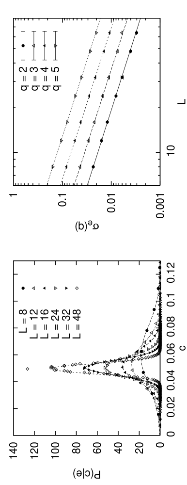
Figure 4: The left figure shows the conditinal distribution $P(c|e)$ at $e=(1-1/(1+\sqrt{q}))/L^{2}$, i.e. the critical link density, for the $q=3$ model. The right figure shows the width of the distribution $P(c|e)$ as a function of $L$, all the curves show a $L^{-1}$ decay. The curves for $q\geq 3$ have been shifted for clarity.

In the RC model each cluster can be in $q$ different configurations, hence we get an additive entropy contribution of $\ln q$ from every cluster. Consequently we see that for a fixed number of links the average number of clusters will increase with $q$. On the other hand larger amount of entropy per cluster, means that for high $q$ entropy will dominate the competetion between internal energy and entropy at a lower number of clusters, and consequently at the critical point $\langle\mathsf{C_{\mathcal{}}}\rangle$ decreases with increasing $q$. These points are illustrated in Fig. 5.

Figure 5: The mean number density of clusters as a function of $q$, for a fixed density of links and at the ($q$ dependant) critical link density. The results in the figure are from a $16\times 16$ lattice.

4.3 Evaluation of the Tutte polonymial

The Tutte polynomial can be defined in terms of a recursive definition[13]; which immediately leads to a simple and exact algorithm for computation of $T_{\mathcal{G}}(x,y)$. However this algorithm has exponential complexity, and is clearly not feasible for anything but very small graphs. Due to it’s importance in many different areas of mathematics and computer science, this has lead to a large effort to find efficient approximate algorithms for evaluation of the Tutte polynomial[23].

Using the algorithm presented here we can also estimate Tutte polynomials, in Fig. 6 we show the reliability polynomial and the Chromatic polynomial. With the current approach the running time to determine the Tutte polynomial is governed by the running time of the MC algorithm, and at least for $q\leq 4$ the Swendsen-Wang algorithm is rapidly mixing[24].

Figure 6: The reliability polynomial Eq. 4 and chromatic polynomial Eq. 5 for a $3\times 3$ lattice. The solid lines are exact results from the computer algebra system Maple, and the points come from our simulations. The very small system size considered is to limit the run-time of Maple

When the arguments $x,y$ of the Tutte polynomial move a long way away from the values used when sampling, the results become unreliable; consult Eq. 6 to see how $x$ and $y$ are related to the parameters $q$ and $\beta$ of the Potts model. In particular for $x<1$ and/or $y<1$ the evaluation of $T(x,y)$ is difficult, because in these regions the polynomial terms are oscillating and inaccurate coefficients lead to large relative errors.

4.4 Zeros in the complex $q$ plane

The formulation of the partition function as a polynomial in $q$ allows for quite easy evaluation of the zeros of the partition function in the complex $q$ plane. Properties of the complex $q$ zeroes have been investigated both analytically, and numerically[25]. According to the Yang-Lee view of critical phenomena the critical point is characterized by zeros in the complex $\beta$ plane pinching the real axis. The phase transition in the Random Cluster model can be driven by both $\beta$ and $q$, we should therefor see the same pinching of the real $q$ axis.

The critical coupling is given by $\beta_{c}J=\ln(1+\sqrt{q})$, alternatively we find that for a fixed $\beta$ the critical $q$ is given by

$$q_{c}=\big{(}e^{\beta J}-1\big{)}^{2}=v^{2}.$$ (16)

For the current discussion the temperature variable $v$, first introduced in Eq. 6 will be the most convenient. Plotting the zeros of $Z(v,q)$ we expect the zeros to pinch the real $q$ axis close to the $q_{c}$ given by Eq. 16, Fig. 7 shows the distribution of zeros in the complex $q$ plane for two different couplings.

Figure 7: The roots in the complex $q$ plane of the partition function $Z(v,q)$ at couplings $v=\sqrt{3}$ (top) and $v=\sqrt{5}$ (bottom). We observe that the zeroes close in on the critical $q$ values of 3 and 5.

If we denote the zero closest to $q_{c}$ with $q_{c}(L)$, we find that $q_{c}(L)$ converges towards $q_{c}$ with increasing system size. To determine which zero is indeed the “critical” one we have measured distance $d(q_{i},q_{c})$ using both the ordinary metric $d_{2}(x,y)=|x-y|$ and also $d_{1}(x,y)=|\mathrm{Im}(x)-\mathrm{Im}(y)|$. For $v^{2}\lesssim 3.0$ the two methods select the same zero, whereas for $v^{2}\gtrsim 3.0$ different zeros are selected, and the real part of the zero selected by $d_{2}$ jumps about randomly. Fig. 8 shows finite size scaling plots of the $|\mathrm{Im}(q)|$ (as determined by using $d_{1}$) for the zero closest to the real $q$ axis. This should scale as

$$|\mathrm{Im}(q)|\sim L^{-\frac{1}{\nu}}.$$ (17)

For $q=2$ and $q=3$ this gives $\nu\approx 0.992(7)$ and $\nu\approx 0.863(7)$ which agree reasonably well with the exact values of $1$ and $5/6\approx 0.8333\ldots$. For $q=4$ we get $\nu\approx 0.77(3)$, this is well above the exact value of $2/3$ + logarithmic corrections. If we assume an effective exponent for the first order transition at $q=5$ we would expect $\nu=1/2$, whereas the estimated value is $\nu=0.77(6)$.

The reason that the quality of the $\nu$ estimates detoriate with increasing $q$ is probably that the slope of the curve $\beta_{c}(q)$ is reduced with increasing $q$. When the transition is driven by $q$ the critical point is approached more and more tangentially. It seems reasonable that this makes a precise determination of the critical properties progressively more difficult. Furthermore the model has limiting behaviour at $q=4$, with strong corrections to scaling; consequently critical properties are notoriously difficult to determine numerically at $q=4$[26].

Figure 8: The plots show $|\mathrm{Im}(q)|$ for the zero closest to the real axis, as a function of system size $L$. The value of $v^{2}$ coincides with $q_{c}$. The error bars are generally smaller than the symbol size. The solid lines are least squares fits with slope, from top to bottom, $-1.3(1),-1.29(5),-1.159(9),-1.008(7).$

The zeroes are found using the MPSolve[27] package. To determine the roots of $Z(v,q)$ in the complex $q$ plane is an ill-posed problem. Firstly the coefficeints $a_{C}(p)$ (see Eq. 7) vary over a wide range, secondly finite sampling statistics adds to the problem. In particular the states with $\mathsf{C_{\mathcal{}}}\to N$ are typically not sampled at all. For independent simulations the pattern of zeroes differs significantly from case to case, however the location of the zero $q_{c}(L)$ shows much less fluctuations. The results in Fig. 8 are the total of ten independent simulations, and as we see the error bars are very small.

In a large paper by Alan Sokal[25] it is shown that the complex $q$ zeros of the partition function $Z(v,q)$ for $|1+v|\leq 1$ are all located within a circle given by the maximal degree of the graph. The restriction $|1+v|\leq 1$ corresponds to the antiferromagnetic Potts model, which is not what we have considered in this paper. If the restriction $|1+v|\leq 1$ is relaxed the radius is found to scale as (for spatially constant $v$)

$$R_{q}\sim\max\left[v,v^{r/2}\right],$$ (18)

where $r$ is the maximum degree of the graph, i.e. the maximum number of edges incident on any one vertex. For an ordinary cubic lattice in two dimensions we have $r=4$, hence we expect to see a crossover from $v$ to $v^{2}$ scaling around $v=1$. Fig. 9 shows the radius $R_{q}$ as a function of $v$.

Figure 9: The radius $R_{q}$ for a two dimensional square lattice, i.e. $r=4$. The solid line is $f(v)\sim a\cdot v$ and the dashed line is $g(v)\sim a+b\cdot v^{2}$.

5 Conclusion

We have shown that the nontrivial information of the Potts model is contained in the density $\Gamma_{\mathcal{G}}({\mathsf{C_{\mathcal{}}}},\mathsf{E_{\mathcal{}}})$, and this is independent of $q$. $\Gamma_{\mathcal{G}}({\mathsf{C_{\mathcal{}}}},\mathsf{E_{\mathcal{}}})$ is purely combinatorial/geometric property of the underlying lattice, emphasizing the connection between these concepts and critical phenomena. Furthermore we have devised an algorithm to estimate $\Gamma_{\mathcal{G}}({\mathsf{C_{\mathcal{}}}},\mathsf{E_{\mathcal{}}})$ from Monte Carlo simulations, and used this to study various properties of the Potts / Random Cluster model.

References

References

- [1] F. Y. Wu. The potts model. Rev. Mod. Phys., 54:235–268, 1982.
- [2] R. J. Baxter. Potts model at the critical temperature. J. Phys. C, 6:445, 1973.
- [3] B. Nienhuis, A. N. Berker, E. K. Riedal, and M. Schick. First- and second-order phase transitions in potts models: Renormalization-group solution. Phys. Rev. Lett, 43:737, 1979.
- [4] Alexander K. Hartmann. Calculation of partition functions by measuring component distributions. Phys. Rev. Lett., 94:050601, 2005.
- [5] C. M. Fortuin and P .W. Kasteleyn. On the random-cluster model : I. Introduction and relation to other models. Physica, 57:536, 1972.
- [6] H.W.J. Blöte and M. P. Nightingale. Critical behaviour of the two-dimensional potts model with a continuous number of states; a finite size scaling analysis. Physica A, 112:405, 1982.
- [7] Ferdinando Gliozzi. Simulation of potts models with real and no critical slowing down. Phys. Rev. E, 66(016115), 2002.
- [8] Youjin Deng, Henk W.J. Blöte, and Bernard Nienhuis. Backbone exponents of the two-dimensional q-state potts model: A monte carlo investigation. Phys. Rev. E, 69:026114, 2004.
- [9] Martin Weigel, Wolfhard Janke, and Chin-Kun Hu. Random-cluster multihistogram sampling for the q-state potts model. Phys. Rev. E, 65(036109), 2002.
- [10] Robin J. Wilson. Introduction to graph theory. Longman Scientific & Technical, 1985.
- [11] W. T. Tutte. A contribution to the theory of chromatic polynomials. Can. J. Math, 6:80–91, 1954.
- [12] T. H. Brylawski and J. G. Oxley. The tutte polynomial and its applications. In N. White, editor, Matroid Applications, pages 123–225. Cambridge University Press, 1992.
- [13] D.J. A. Welsh. Complexity: Knots, Colourings and Counting. Cambridge University Press, 1993.
- [14] Robert G. Edwards and Alan D. Sokal. Generalization of the fortuin-kasteleyn-swendsen-wang representation and monte carlo algorithm. Phys. Rev. D, 38:2009, 1988.
- [15] R. H. Swendsen and J.-S. Wang. Non-universal critical dynamics in monte carlo simulations. Phys. Rev. Lett., 58:86, 1987.
- [16] D. J. A. Welsh. Computational complexity of problems in statistical physics. In G. R. Grimmet and D. J. A. Welsh, editors, Disorder in Physical Systems A volume in Honour of John M. Hammersley, pages 307–321. Oxford Science Publications, 1990.
- [17] Mark Jerrum and Alistair Sinclair. The markov chain monte carlo method: an approach to approximate counting and integration. In D.S.Hochbaum, editor, Approximation Algorithms for NP-hard Problems, pages 482–520. PWS Publishing, Boston, 1996.
- [18] Mark R. Jerrum and Allistair J. Sinclair. Approximating the permanent. SIAM Journal on Computing, 18:1149–1178, 1989.
- [19] Mark Jerrum and Alistair Sinclair. Polynomial-time approximation algorithms for the ising model. SIAM Journal on Computing, 22:1087–1116, 1993.
- [20] A. M. Ferrenberg and R. H. Swendsen. xxx. Phys. Rev. Lett, 63:1195, 1989.
- [21] Nelson A. Alves, Bernd A. Berg, and Ramon Villanova. Ising-model monte carlo simulations: Density of states and mass gap. Phys. Rev. B, 41:383–394, 1990.
- [22] J. Hove. Density of states from monte carlo simulations. Phys. Rev. E, 70:056707, 2004.
- [23] Noga Alon, Alan M. Frieze, and Dominic Welsh. Polynomial time randomized approximation schemes for tutte-gröthendieck invariants: The dense case. Random Struct. Algorithms, 6(4):459–478, 1995.
- [24] Vivek K. Gore and Mark R. Jerrum. The swendsen-wang process does not always mix rapidly. Journal of Statistical Physics, 97(1-2):67–86, 1999.
- [25] Alan D. Sokal. Bounds on the complex zeros of (di)chromatic polynomials and potts-model partition functions. Comb.Probab.Comput., 10:41–77, 2001.
- [26] Jesús Salas and Alan D. Sokal. Logarithmic corrections and finite-size scaling in the two-dimensional 4-state potts model. J. Stat. Phys., 88:567–615, 1997.
- [27] D. A. Bini and G. Fiorentino. Design, analysis and implementation of a multiprecision polynomial rootfinder. Numerical Algorithms, 23:127–173, 2000.