Nonlinear Ionic Conductivity of Thin Solid Electrolyte Samples: Comparison between Theory and Experiment

Abstract

Nonlinear conductivity effects are studied experimentally and theoretically for thin samples of disordered ionic conductors. Following previous work in this field the experimental nonlinear conductivity of sodium ion conducting glasses is analyzed in terms of apparent hopping distances. Values up to 43 Å  are obtained. Due to higher-order harmonic current density detection, any undesired effects arising from Joule heating can be excluded. Additionally, the influence of temperature and sample thickness on the nonlinearity is explored. From the theoretical side the nonlinear conductivity in a disordered hopping model is analyzed numerically. For the 1D case the nonlinearity can be even handled analytically. Surprisingly, for this model the apparent hopping distance scales with the system size. This result shows that in general the nonlinear conductivity cannot be interpreted in terms of apparent hopping distances. Possible extensions of the model are discussed.

I Introduction

One important method for improving the properties of solid ionic conductors with regard to applications in microbatteries, fuel cells and electrochromic devices is the preparation of thin films Noda et al. (2004); Appetecchi et al. (2003); Jonghe et al. (2003); Lu et al. (2002); Rowley and Mortimer (2002); Tarascon and Armand (2001); Murray and Barnett (1999); Croce et al. (1998). Both the electrical resistance and the mechanical stiffness of the film decrease with decreasing thickness. The decrease of the electrical resistance is important for improving the power density of microbatteries, the efficiency of fuel cells and the switching time of electrochromic devices. A low mechanical stiffness leads to a better processibility of the film.

For the integration of a thin film into a lithium microbattery, an electrochemical window in which the film is stable from 0-5 V is required Tarascon and Armand (2001); Noda et al. (2004). The application of 5 V to samples with thicknesses of 100 nm and less leads to high electric field strengths in the samples, which result in field-dependent ion transport effects. Generally, the ionic conductivity of solid electrolytes increases with increasing field strength Hyde and Tomozawa (1986); Barton (1996); Isard (1996); Tajitsu (1996, 1998). Thus, field-dependent ion transport is of potential interest for improving the applicability of thin-film electrolytes.

Mathematically, the field-dependent electrical properties of thin solid electrolyte samples can be described by:

$$j_{dc}(E_{dc})=\sigma_{1,dc}\;E_{dc}+\sigma_{3,dc}\;E^{3}_{dc}+\sigma_{5,dc}\;E^{5}_{dc}+...$$ (1)

Here, the linear dependence of the dc current density $j_{dc}$ on the dc electric field $E_{dc}$ at low field strengths is characterised by the low-field dc conductivity $\sigma_{1,dc}$, while the nonlinear dependence at high field strengths is characterised by the higher-order conductivity coefficients $\sigma_{3,dc}$, $\sigma_{5,dc}$ etc.

A first step to interpret the nonlinearity of the conductivity is to consider a simple regular hopping model with distance $a$ between adjacent sites. For this model it turns out that

$$j_{dc}(E_{dc})\propto\sinh(q\beta aE_{dc}/2)$$ (2)

with $\beta=1/k_{B}T$. Thus, in the framework of this model, it is possible to extract the hopping distance $a$ from field-dependent electrical data. Although the model is too simple to provide a realistic description of ion conduction in disordered materials, such as glasses and polymer electrolytes, the $j_{dc}(E_{dc}$) curves of many real ion conductors can be reasonably well fitted by Eq. (2). However, the values obtained for the hopping distance $a$ are much larger than typical distances between neighboring sites in ionic conductors. For instance, in the case of ion conducting glasses, values in the range from 15 Å  to 30 Å  have been found Hyde and Tomozawa (1986); Barton (1996); Isard (1996).

These experimental results are based on measurements using dc electric field. A major drawback of this method is the lack of information about Joule heating effects. Joule heating may lead to an increase of the sample temperature, resulting in an increase of the ionic conductivity. In contrast, the application of ac electric fields allows for a direct differentiation between nonlinear ion transport and Joule heating. Nonlinear ion transport leads to higher harmonic contributions to the current density spectrum, while this is not the case for Joule heating Murugavel and Roling (2004). The field dependence of the higher harmonic contributions can be used to determine values for the higher order–conductivity coefficients $\sigma_{3,dc}$, $\sigma_{5,dc}$ etc. Murugavel and Roling (2004). Thus, by means of nonlinear ac conductivity spectroscopy it is possible to differentiate between the higher-order conductivity coefficients, while the application of dc fields yields only one $j_{dc}(E_{dc}$) curve.

The values $\sigma_{1,dc}$ and $\sigma_{3,dc}$ can be used to define an apparent hopping distance:

$$a_{app}^{2}\equiv 24\sigma_{3,dc}/(\sigma_{1,dc}\,q^{2}\,\beta^{2})$$ (3)

This definition of $a_{app}$ implies that for the regular hopping model, the simple relation $a_{app}=a$ holds. However, two of the present authors have shown that for different sodium ion conducting glasses, the apparent hopping distances $a_{app}$ are in a range from 39Å  to 55Å  Murugavel and Roling (2004). Thus, the calculation of $a_{app}$ by means of Eq. (3) leads to higher values than fits of $j_{dc}(E_{dc}$) data by means of Eq. (2). This implies that Eq. (2) does not provide an exact description of the nonlinear conductivity of ionic conductors. This is confirmed by the observation of negative values for $\sigma_{5,dc}$ Murugavel and Roling (2004), whereas the validity of Eq. (2) implies positive values for $\sigma_{5,dc}$.

In this paper, we rationalize these experimental results by considering simple hopping models with strong site and barrier disorder. We find that in the framework of such models, the apparent hopping distance $a_{app}$ is, indeed, considerably larger than the distance $a$ between adjacent sites. However, $a_{app}$ shows an unexpected dependence on the thickness of the model systems in the direction of the applied electric field. In order to check whether also real ionic conductors exhibit such a thickness dependence of their nonlinear electrical properties, we have carried out nonlinear ac conductivity measurements on ion conducting glass samples of different thickness. We compare theoretical and experimental results, and we discuss implications of these results for further theoretical and experimental work.

II Theory

First, we consider a general 1D-hopping model with site and barrier disorder; see Fig. 1. The individual $N$ sites are characterized by energies $E_{i}$. With an external field the hopping rates for leaving site $i$ are $\Gamma_{i,\pm}$ where the sign denotes whether the hopping is along (+) or opposite (-) to the field. The field dependence of $\Gamma_{i,\pm}$ can be expressed as $\Gamma_{i,\pm}(u)=\exp(\pm u)\gamma_{i,\pm}$ with

$$u=q\beta aE_{dc}/2.$$ (4)

Correspondingly, $\gamma_{i,\pm}$ are the hopping rates without applied field. Detailed balance requires $\gamma_{i,+}/\gamma_{i+1,-}=\exp(-\beta(E_{i+1}-E_{i}))$. To get a stationary long-time solution for the current, periodic boundary conditions are used. Physically, this reflects the interaction of both electrodes via the voltage source.

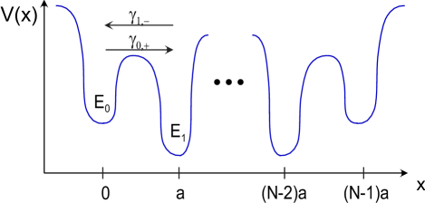
Figure 1: Sketch of the 1D hopping model, used in the theoretical analysis. Periodic boundary conditions are employed. The model is point symmetric.

The time evolution of the single-particle problem is governed by the rate equations

$$(d/dt)p_{i}(t) =-\Gamma_{i,+}(u)p_{i}(t)-\Gamma_{i,-}(u)p_{i}(t)$$ (5)

$$+\Gamma_{i-1,+}(u)p_{i-1}(t)+\Gamma_{i+1,-}(u)p_{i+1}(t).$$

The stationary long-time solutions are denoted as $p_{i}^{\infty}(u)$. The argument expresses their dependence on the electric field. Finally the current $j_{dc}(u)$ in the long-time limit can be written as

$$j_{dc}(u)/(qa)\equiv\tilde{j}(u)=p_{i}^{\infty}(u)\Gamma_{i,+}(u)-p_{i+1}^{\infty}(u)\Gamma_{i+1,-}(u).$$ (6)

Note that the current between all pairs of sites is identical. Therefore $\tilde{j}(u)$ and thus $j_{dc}(u)$ do not depend on the index $i$.

This property can be used to solve the system of equations analytically for arbitrary $N$; see Refs. Ambegaokar and Halperin (1969); Derrida (1983); Bouchaud and Georges (1990); Kehr et al. (1997) for detailed information.

Using a notation which is appropriate for our further analysis the solution can be written as

$$\tilde{j}(u)=(\exp(Nu)-\exp(-Nu))/B$$ (7)

with

$$B=\sum_{m=0}^{N-1}A_{m}\exp((1-N+2m)u).$$ (8)

The disorder is contained in

$$A_{m}=\sum_{i=0}^{N-1}f(m,i)$$ (9)

with

$$f(m,i)\equiv\exp(-\beta(E_{i+m}-E_{i}))/\gamma_{i,-}.$$ (10)

In case that the disorder of adjacent sites is uncorrelated one obtains $\langle A_{1}\rangle=...=\langle A_{N-2}\rangle\equiv b_{1}$ and $\langle A_{0}\rangle=\langle A_{N-1}\rangle=b_{0}$, where the brackets denote the disorder average. Please note that $\langle A_{m}\rangle$ as a sum of $N$ terms trivially scales like $N^{1}$.

In what follows we consider the situation that the energy landscape is point symmetric. In this way one can guarantee that in analogy to the experimental situation the current only depends on odd powers of the electric field. In particular one strictly has $A_{m}=A_{N-1-m}$.

Here we are interested in a Taylor-expansion of $\tilde{j}(u)$ with respect to $u$. Expansion of the numerator and the denominator yields

$$\tilde{j}(u)=\frac{2Nu+N^{3}u^{3}/3+...}{\sum_{m}A_{m}+(1/2)\sum_{m}A_{m}(-N+1+2m)^{2}u^{2}+...}.$$ (11)

Reordering of terms yields up to order $u^{2}$

$$\tilde{j}(u)=\frac{2Nu}{\sum A_{m}}\left[1+u^{2}\left(N^{2}/6-\frac{\sum_{m}A_{m}(-N+1+2m)^{2}}{2\sum_{m}A_{m}}\right)\right].$$ (12)

From this the low-field conductivity $\sigma_{1,dc}$ can be written as:

$$\frac{\sigma_{1,dc}}{q^{2}\beta a^{2}}=\left\langle\frac{N}{\sum_{m}A_{m}}\right\rangle.$$ (13)

The brackets denote the average over the disorder.

In a first step we use the property that in the thermodynamic limit $N\rightarrow\infty$ one has

$$\left\langle\frac{1}{\sum_{m}A_{m}}\right\rangle=\frac{1}{\langle\sum_{m}A_{m}\rangle}.$$ (14)

This relation is derived in the Appendix.

With the same arguments one can replace in the disorder average of $\tilde{j}(u)$ in Eq. (12) all terms $\sum_{m}A_{m}$ by $\langle\sum_{m}A_{m}\rangle$. Combining Eq. (3) with Eq. (12) and using this preaveraging of $\sum_{m}A_{m}$ one obtains in the limit of large $N$ the following relation for $a^{2}_{app}$:

$$a^{2}_{app}/a^{2}=N^{2}-\frac{3\sum_{m}\langle A_{m}(-N+1+2m)^{2}\rangle}{\langle\sum_{m}A_{m}\rangle}.$$ (15)

Straightforward calculation yields

$$\langle\sum_{m}A_{m}\rangle=Nb_{1}+2(b_{0}-b_{1})$$ (16)

and

$$\langle\sum_{m}A_{m}(-N+1+2m)^{2}\rangle = (1/3)b_{1}(N^{3}-N)$$ (17)

$$+ 2(b_{0}-b_{1})(N-1)^{2}$$

Expansion of the denominator with respect to $1/N$ finally yields

$$a^{2}_{app}/a^{2}=1+4N(b_{1}-b_{0})/b_{1}.$$ (18)

This shows that for large $N$ one finds the scaling relation $a^{2}_{app}\propto N$.

What is the origin of the $N$-dependence? In the case of vanishing disorder one has $p_{i}^{\infty}(u)=1/N$ for all $u$. Thus the $u$-dependence of the current $\tilde{j}(u)$, see Eq. (6), exclusively results from the trivial $u$-dependence of the rates $\Gamma_{i,\pm}(u)$ and gives rise to $a^{2}_{app}/a^{2}=1$. In contrast, for disorder one also obtains contributions from $p_{i}^{\infty}(u)$. After solving the N linear equations, characterizing the stationary case, the expansion of $p_{i}^{\infty}(u)$ with respect to $u$ contains terms proportional to $N$, which are responsible for the $N$-dependence of $a^{2}_{app}/a^{2}$. For the N-dependence of the $\sigma_{i,dc}$ one finds $\sigma_{1,dc}\propto N^{-1}$ and $\sigma_{3,dc}\propto N^{0}$, thus giving rise to $a^{2}_{app}\propto\sigma_{3,dc}/\sigma_{1,dc}\propto N$. The scaling of $\sigma_{1,dc}$ simply means that the conductivity is proportional to the particle concentration, i.e. $1/N$. Actually, it is also possible to calculate $\tilde{j}(u)$ for fixed $u$ in the thermodynamic limit, thereby revealing non-analytical behavior for $u=0$. This discussion, however, is beyond the scope of the present paper.

It may be instructive to calculate $b_{0}$ and $b_{1}$ for different types of disorder. In case of a random barrier model for which all $E_{i}$ are constant one obtains $b_{0}=b_{1}$ and thus $a^{2}_{app}/a^{2}=1$. In case of pure energetic disorder we choose a model for which $E_{i}$ is either $e$ or $0$, both with 50% probability. Then one finds numerically in the low-temperature limit $u\gg 1$ that $b_{0}\approx 0.24\exp(\beta e)$ and $b_{1}\approx 0.37\exp(\beta e)$. For large $N$ one thus gets $a_{exp}^{2}/a^{2}\approx 1.5N$.

In Fig. 2 we show the asymptotic result Eq. (18) for $a^{2}_{app}/a^{2}$ together with the exact result, obtained from averaging the current in Eq. (12) and finally calculating $a^{2}_{app}/a^{2}$ from Eq. (3). One can see that for $N\geq 40$ the large-N limit works very well. For smaller $N$ the apparent jump length is smaller than expected. We mention in passing that all data points have been obtained from averaging over 10000 realisations of the disorder. This large number is necessary because numerically it turns out that the standard deviation for the distribution of $a^{2}_{app}/a^{2}$ is of the same order as $a^{2}_{app}/a^{2}$ itself (for all $N$). The main conclusion is that for larger values of $N$ also large values of $a^{2}_{app}/a^{2}$ can be realized. Furthermore we have included data for $u=2$ in Fig. 2. Decrease of $u$ corresponds to an increase of temperature. In agreement with the experimental data (see below) one finds that $a^{2}_{app}/a^{2}$ decreases with increasing temperature. Of course, for $u=0$, one obtains $a^{2}_{app}/a^{2}=1$. Actually, as seen from Fig. 2 the asymptotic result is not strictly linear as naively expected from Eq. (18). The reason is that for small $N$ also the values of $b_{0}/N$ and $b_{1}/N$ somewhat depend on $N$ due to finite-size effects.

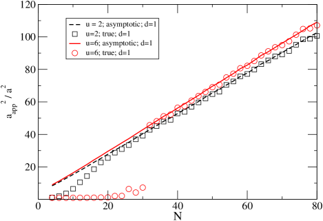
Figure 2: Comparison of the numerical solution for $a_{app}$ with the asymptotic analytical solution.

So far we have considered a single particle in a disordered potential. In recent work it has been shown Lammert et al. (2003); Habasaki and Hiwatari (2004); Vogel (2004) that it is a more realistic picture to consider the dynamics of a vacancy rather than a particle. Not surprisingly, the new set of equations is very similar and the results for $a^{2}_{app}/a^{2}$ turn out to be identical.

A more serious deviation from the experimental situation is the dimensionality. To which degree can the results for the 1D model be generalized to systems with more than one dimension? To clarify the influence of the dimension we have extended the model to two dimensions, also using periodic boundary conditions in the second dimension. We define $N_{o}$ as the number of sites orthogonal to the field. The set of rate equations for the 1D case can be easily generalized. Solving for the stationary long-time solution is equivalent to solve a system of linear equations with $N\cdot N_{o}$ variables. Unfortunately, it is not possible to solve the multidimensional case analytically in the way it has been done for the 1D system. Therefore the solution is purely numerical. After averaging over the disorder one obtains the results, shown in Fig. 3. Two important conclusions can be drawn from these results:(i) The scaling $a^{2}_{app}/a^{2}\propto N$ also holds for two-dimensional systems, albeit only for somewhat larger $N$ (as can be seen for $N_{o}=20$). (ii) The absolute value of $a^{2}_{app}/a^{2}$ strongly decreases with increasing $N_{o}$. Comparing $N_{o}=10$ and $N_{o}=20$ one may speculate that $a^{2}_{app}/a^{2}\propto N/N_{o}$.

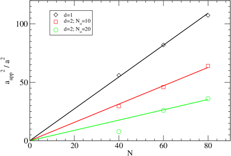
Figure 3: Dependence of $a_{app}$ on the size parallel and orthogonal to the electric field.

III Experimental

For the nonlinear ac conductivity measurements, we prepared samples of the glasses 0.25 Na₂O $\cdot$ 0.096 CaO $\cdot$ 0.062 Al₂O₃ $\cdot$ 0.592 SiO₂ (NCAS25) and 0.25 Na₂O $\cdot$ 0.75 SiO₂ (NS25) with different thicknesses. The preparation of the NCAS25 glass is described in Ref. Murugavel and Roling (2004). The NS25 glass was prepared by using the same procedure.

The experimental setup for nonlinear conductivity spectroscopy and the high-voltage measurement system are described in detail in Ref. Murugavel and Roling (2004). An important aspect of our method is the utilisation of nonblocking electrodes consisting of highly conducting NaCl solutions. Thereby, we avoid (i) electrochemical reactions at the electrode/sample interfaces and (ii) electron or hole injection into the sample. The measurements were carried out in a frequency range from 10 mHz to 10 kHz with a maximum voltage amplitude of 500 V.

IV Results

For the NCAS25 glass, the third-order conductivity coefficients $\sigma_{3,dc}$ were derived from an analysis of the higher harmonic components of the current density spectrum as described in Ref. Murugavel and Roling (2004). At low frequencies, both the low-field conductivity $\sigma_{1}(\nu)$ and the third-order conductivity coefficient $\sigma_{3}(\nu)$ exhibit plateaus, the plateau values being identical to the bulk dc values, $\sigma_{1,dc}$ and $\sigma_{3,dc}$ Murugavel and Roling (2004). From these dc values, the apparent jump distance $a_{app}$ were calculated using Eq. (3). A careful analysis of the frequency dependence of the conductivity data revealed, however, that in the low-frequency region, sample/electrode interface impedances have a weak influence on the conductivity. This will be discussed later in more detail for the NS25 glass where the interfacial impedance effects are more pronounced. For the determinination of $\sigma_{1,dc}$ and $\sigma_{3,dc}$ of the NCAS25 glass, the analysis was limited to a frequency regime where the interfacial impedance was less than 1% of the overall impedance. Due to the narrower frequency regime, the values obtained for $a_{app}$ were a few percent lower than those published in Ref. Murugavel and Roling (2004). In Fig. 4 we show a plot of $a_{app}$ versus temperature T for two NCAS25 glass samples with thicknesses 65 $\mu$m and 85 $\mu$m. Within the experimental error, we do not detect a significant thickness dependence of $a_{app}$.

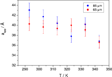
Figure 4: Apparent jump distance of mobile Na⁺ ions, $a_{app}$, in NCAS25 glass samples with different thicknesses.

In the case of the NS25 glass, we carried out measurements on samples with thicknesses 83 $\mu$m, 100 $\mu$m and 120 $\mu$m. Unfortunately, for all samples, the higher harmonic current density $j^{\prime}(3\nu)$ did not exhibit well-defined low-frequency plateaus. As an example, we show in Fig. 5 results for the base current density $j^{\prime}(\nu)$ (closed symbols) and for the higher harmonic current density $j^{\prime}(3\nu)$, measured after applying an ac field with amplitude $E_{0}$ = 41.6 kV/cm to a sample with thickness $d$ = 120 $\mu$m. Both $j^{\prime}(\nu)$ and $j^{\prime}(3\nu)$ are normalised by the field amplitude $E_{0}$ and are plotted versus frequency at two different temperatures $T$ = 303 K and 313 K. While a bulk dc plateau in $j^{\prime}(\nu)$ is clearly detectable, the higher harmonic current density $j^{\prime}(3\nu)$ exhibits a frequency dependence over the entire frequency range. Therefore, it was not possible to obtain accurate values for $\sigma_{3,dc}$ of this glass.

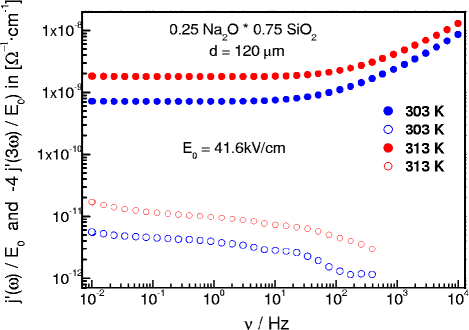
Figure 5: Base current density $j^{\prime}(\nu)$ (closed symbols) and higher harmonic current density $j^{\prime}(3\nu)$ (open symbols), measured after applying an ac field with amplitude $E_{0}$ = 41.6 kV/cm to the NS25 glass. Both Fourier components of the current density are normalised by the field amplitude $E_{0}$ and are plotted versus frequency $\nu$ at two different temperatures, $T$ = 303 K and 313 K. In addition, the quantity $j^{\prime}(3\nu)/E_{0}$ is multiplied by a factor of -4.

The reason for the absence of well-definded dc plateaus in $j^{\prime}(3\nu)$ are most likely electrical impedances at the sample/electrode interfaces. Although we use highly conducting liquid NaCl solutions as electrodes, we detect significant interfacial impedances at low frequencies, which are related to additional barriers for the diffusion of the sodium ions from the glass samples into the NaCl solution and vice versa. As an example, we show in Fig. 6 plots of the imaginary part of the impedance and of the real part of permittivity versus frequency for the NS25 glass. The data were obtained at $T$ = 313 K and different applied voltages. At high frequencies, the impedance and permittivity data are determined by ionic conduction in the bulk and exhibit only a weak voltage dependence. However, below 1 Hz, additional impedance contributions from the sample/electrode interfaces are detected. These interfacial impedances decrease strongly with increasing voltage. However, even at the highest applied voltages, interfacial impedance contributions are still present.

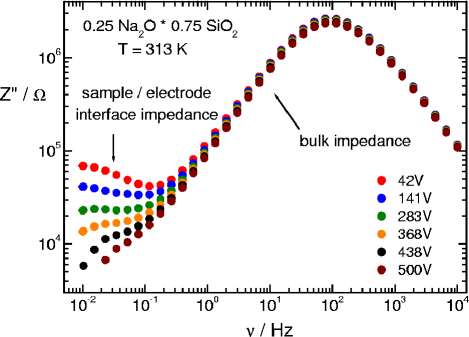
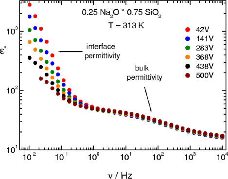
Figure 6: Frequency dependence of the imaginary part of the impedance, $Z^{\prime\prime}$ and of the real part of the permittivity, $\varepsilon^{\prime}$, for the NS25 glass. The data were taken at $T$ = 313 K and different voltage amplitudes. Above 1 Hz, the spectra are determined by bulk ionic conduction, while below one 1 Hz, sample/electrode interface impedances govern the frequency and field dependence of the electrical data. The interfacial impedances are related to additional barriers for the diffusion of the sodium ions from the glass samples into the NaCl solution and vice versa.

V Discussion

Although we did not detect a significant thickness dependence of the apparent hopping distance $a_{app}$ for the NCAS25 glass, our experimental results do not completely rule out such a thickness dependence. For an unambiguous prove or disprove we will have to study samples with a broader range of thicknesses. In the case of the NS25 glass, the thickness was varied by about 50%, however unfortunately, accurate $\sigma_{3,dc}$ values for this glass could not be obtained, most likely due to sample/electrode interface impedance contributions to $j^{\prime}(3\nu)$.

It is remarkable that the interfacial impedances persist up to voltages of several hundred volts. A voltage drop of the order of 100 V in an extremely thin interface region should lead to enormously high electric fields which should pull the ions over the interfacial barriers. When we assume that the thickness of the interfacial region is of the order of 10 nm, a voltage drop of the order of 100 V in this region leads to field strengths of the order of 100 MV/cm. This is even far above the electrical breakdown strengths of ion conducting glasses.

From this we conclude that the interfacial regions causing the interfacial impedance effects must be much thicker than 10 nm. A possible explanation is the build-up of a resistive surface layer due to water corrosion. It is thinkable that water diffuses from the NaCl solution into the glass and and changes the chemical structure close to the surface by breaking Si-O-Si bonds and forming Si-O-H groups Tomozawa (1985). The thickness of such chemically modified surface layers may be much larger than 10 nm Tomozawa (1985). This assumption would explain the more pronounced interfacial impedance effects in the case of the NS25 glass. It is well known that the chemical corrosion of simple alkali silicate glasses is much faster than that of technical silicate glasses containing additional alkaline-earth oxides. If the assumption is correct, the interfacial impedances should be avoidable by using non-aquaous salt solutions, based for instance on glycerol. This will be the subject of further experiments.

From a theoretical point of view, the observation of large values of $a_{app}$ has been reproduced by a simple model, describing the hopping dynamics of a particle (or vacancy) in a disordered model potential. In the 1D case it is even possible to solve the problem analytically. This simple and well-studied model contains the surprising property that $a_{app}$ scales with the thickness. Identification of $a_{app}\equiv(24\sigma_{3,dc}/q^{2}\beta^{2}\sigma_{1,dc})^{1/2}$ as some kind of effective hopping distance was motivated by the solution of the regular model. The scaling property $a_{app}\propto aN^{1/2}$ for the disordered hopping model directly implies, however, that this interpretation is not justified. Formally, this can be traced back to the fact that the field-dependence of the current in the disordered case is not only goverened by the new transition rates $\Gamma_{i,\pm}$ but also by the modified populations; see Eq. 6. Rather for this model the value $a_{app}/(aN^{1/2})$ expresses information about the nature of the disorder; see Eq. (18). Thus, the experimental observation of $a_{app}\approx 50$Å  does not contradict the generally accepted idea that typical hopping distances in ion conductors should be smaller than, let’s say, 10Å.

VI Conclusions

Combining a detailed experimental analysis with a thorough model calculation several new aspects have been elucidated. (i) The large values for $a_{app}$ in thin samples is not related to Joule heating, but is indeed a reproducible property of the ion dynamics. (ii) These values increase with decreasing temperature. (iii) The large values of $a_{app}$ as well as the temperature dependence can be rationalized by a simple hopping model. (iv) In general, $a_{app}$ cannot be interpreted as an apparent hopping distance.

Many new and important questions have emerged from the present results. (1) What is the real physical interpretation of $a_{app}$? In particular it would be helpful to relate this quantity to equilibrium properties of the system Dyre (1989); Dieterich (1998). (2) Is is possible to refine the model to get a limiting value for $a_{app}$? One may speculate that consideration of interaction effects between different particles or holes, respectively, may yield such an upper limit. (3) Do large electric fields also modify the properties of the network and thus indirectly also the ion dynamics? The latter effect has not been included in the modelling. In principle this question could be answered by performing appropriate molecular dynamics simulations of ion conductors. (4) Are experimental values for $a_{app}$ different for crystalline materials as compared to disordered materials? The hopping model, analyzed in this work, might suggest some difference.

Appendix

We consider the covariance of $A_{k}$ and $A_{m}$ which can be written as

$$cov(A_{k},A_{m})=\sum_{i,j}[\langle f(k,i)f(m,j)\rangle-\langle f(k,i)\rangle\langle f(m,j)\rangle].$$ (19)

Closer inspection of the $f(k,i)$ (see Eq. (10)) shows that for extreme disorder the first term is particularly large if $i=j$. This can be seen from the fact that without the additional exponential factor in Eq. (10) one would strictly have $\langle f(k,i)f(m,j)\rangle-\langle f(k,i)\rangle\langle f(m,j)\rangle=0$ for $i\neq j$. As a consequence one can write $cov(A_{k},A_{m})$ as a sum of $N$ terms of similar magnitude such that $cov(A_{k},A_{m})\propto N$. Thus the variance of $\sum_{m}A_{m}$ which can be written as $\sum_{k,m}cov(A_{k},A_{m})$ scales like $N^{3}$. This has to be compared with the scaling $(\sum_{m}A_{m})^{2}\propto N^{4}$. Thus for large $N$ the standard deviation of $\sum_{m}A_{m}$ is much smaller than the value of $\sum_{m}A_{m}$ itself. This justifies Eq. (14).