Transport in one dimensional Coulomb gases: From ion channels to nanopores

Abstract

We consider a class of systems where, due to the large mismatch of dielectric constants, the Coulomb interaction is approximately one–dimensional. Examples include ion channels in lipid membranes and water filled nanopores in silicon films. Charge transport across such systems possesses the activation behavior associated with the large electrostatic self–energy of a charge placed inside the channel. We show here that the activation barrier exhibits non–trivial dependence on the salt concentration in the surrounding water solution and on the length and radius of the channel.

I Introduction

In a number of quasi–one–dimensional systems the interactions between charged carriers follow (for a certain range of distances) the one dimensional Coulomb law: $\Phi(x)\sim|x|$, well known for parallel charged planes. Examples include: ion channels in biological lipid membranes Stryer ; ionchanbook , water–filled nanopores in membranes for desalination devices desalination , water filled nanopores in silicon oxide films Li ; Storm ; Timp , free–standing silicon nanowires Lieber ; Peeters and others. Their common feature is the presence of a quasi 1d channel with the dielectric constant greatly exceeding that of the surrounding 3d media. As a result, the electric field is forced to stay inside the channel, leading to the 1d interaction potential, mentioned above. The purpose of this paper is to study the charge transport through such systems as a function of the carrier concentration, length, temperature, etc. We show that these systems posses very peculiar transport properties, qualitatively different from those found in the examples with shorter range interactions.

To be specific, we focus on the water filled channels. One example is ion channels in lipid membranes. Such a membrane consists of a $L=5\,\mbox{nm}$ thick hydrocarbon layer with the dielectric constant $\kappa_{2}\simeq 2$, surrounded by water with the dielectric constant $\kappa_{1}\simeq 80$. Due to the large ratio $\kappa_{1}/\kappa_{2}\simeq 40\gg 1$ the electrostatic self–energy of a charged ion inside the hydrocarbon layer is huge, making the pure membrane impermeable for ions from water. The only way for ions to cross the membrane is through the water–filled channels formed by proteins embedded into the membrane Stryer ; ionchanbook . Radiuses of such cylindrical channels, $a$, vary from 0.3 to 0.8 nm (we are concerned only with the passive channels without motors).

Another example is a water–filled nanopore made in a silicon film  Li ; Storm . Such nanopore may have the radius $a\simeq 1$ nm and the length $L\simeq 20$ nm. Silicon oxidizes around the channel, giving $\kappa_{2}\simeq 4$. Thus, also in this case $\kappa_{1}/\kappa_{2}=20\gg 1$. Yet another example is provided by water–filled nanopores, say, with $L\simeq 40$ nm and $a\simeq 1.5$ nm in cellulose acetate films used for the inverse osmosis desalination. In this example $\kappa_{2}\simeq 2$ and again $\kappa_{1}/\kappa_{2}=40\gg 1$.

Keeping in mind one of these examples, let us consider a single water filled channel in a macroscopic membrane or a film separating two reservoirs with salty water (Fig. 1a). We assume that walls of the channel do not carry fixed charges. A static voltage $V$, applied between the two reservoirs, drops almost entirely in the channel due to the high conductivity of the bulk solution. One can measure the ohmic resistance, $R$, of the channel as a function of the temperature, $T$, concentration of monovalent salt, $c$ (for example KCl) and parameters of the channel $L$, $a$, $\kappa_{1},\kappa_{2}$. The main goal of this paper is to evaluate $R(T,c,L,a,\kappa_{1},\kappa_{2})$ for the very nontrivial case: $\kappa_{1}\gg\kappa_{2}$. This is a completely classical ($\hbar=0$) problem.

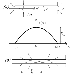
Figure 1: Electric field of a charge in a short (a) and a long (b) cylindrical channel with the large dielectric constant $\kappa_{1}$, in the membrane with the dielectric constant $\kappa_{2}<<\kappa_{1}$. $L$ is the channel length, $a$ is its radius. The self–energy barrier is shown as a function of coordinate $x$ for the case of the short channel. $U_{L}$ is its maximum height. For a long channel $\xi$ is the electric field escape length from the channel.

For a low concentration of salt $c$ the charge transport is due to the rare events, when there is a single (e.g. positive) ion inside the channel. We assume that the radius of the ion, $b$, is smaller than that of the channel $a$, so that the ion is totally surrounded by water. It is easy to see that the electric field of the ion at distances larger than $a$ is deformed because the electric field lines avoid entering the media with the small dielectric constant $\kappa_{2}$ (Fig. 1). This leads to the enhancement of the electrostatic self–energy of the ion, which creates a barrier $U(x)$, where $x\in[-L/2,L/2]$ is the ion coordinate inside the channel. This barrier is the difference between the self–energy of the ion at the point $x$ inside the channel and the self-energy in the bulk. It is the maximum of the barrier, $U(0)=U_{L}$, that determines the resistance of the channel, Fig. 1a.

For a relatively short channel, all field lines are confined inside the channel until they reach its end and go out to the bulk of the water (Fig. 1a). Therefore, the electrostatic self–energy barrier $U_{L}\propto L$ and does not depend on $\kappa_{2}$. On the other hand, in a very long channel (Fig. 1b) the lines eventually escape to the surrounding media with the small dielectric constant $\kappa_{2}$ before they reach the exit to the bulk water. As a result, $U_{L}$ saturates at some value $U_{\infty}$, which depends on the ratio $\kappa_{1}/\kappa_{2}$, but does not depend on the length $L$.

The self–energy barrier was studied by many authors Parsegian ; Lev ; Jordan ; Fink2 ; Fink1 ; Teber . We shall review their results in section II. Here we calculate the barrier for the simplest case of the short channel Fink1 . The electric field $E_{0}$ at a distance $x>a$ from a charge located in the middle of the short channel is uniform and given by the Gauss theorem

$$E_{0}={2\,e\over\kappa_{1}a^{\,2}}\,.$$ (1)

The energy of such field in the volume of the channel determines the maximum height of the barrier (Fig. 1a)

$$U_{L}(0)={e^{2}L\over 2\kappa_{1}a^{\,2}}={eE_{0}L\over 4}\,,$$ (2)

where the zero argument indicates that the result is valid in the limit of vanishingly low salt concentration. For a narrow channel the barrier, $U_{L}(0)$, can be much larger than $k_{B}T$, making the resistance $R$ exponentially large:

$$R\sim\exp\left\{{U_{L}\over k_{B}T}\right\}\,.$$ (3)

In this paper we study what happens when the concentration of the monovalent salt, $c$, in the bulk solution increases and more ions enter the channel. They first arrive as compact neutral pairs of oppositely charged ions. Indeed, such pairs can enter the channel without the self-energy barrier. The one–dimensional character of the electric field between the charges creates a strong confinement between them (Fig. 2).

Figure 2: Electric field of a pair of positive and negative charges inside the channel. When charges move away from each other the energy of the electric field between them grows linearly with the separation.

Indeed, when a pair of oppositely charged ions separates by a distance $x$, the uniform electric field between them, $2E_{0}$, creates the confining “string” potential $\Phi(x)=eE_{0}|x|$. This situation reminds two quarks confined in a meson. Condition $\Phi(x)=k_{B}T$ defines the characteristic thermal length of the pair:

$$x_{T}={k_{B}T\over eE_{0}}={k_{B}T\kappa_{1}a^{\,2}\over 2\,e^{2}}={a^{\,2}\over 2\,l_{B}}\,,$$ (4)

where $l_{B}\equiv e^{2}/(\kappa_{1}k_{B}T)$ is the Bjerrum length (for water at the room temperature $l_{B}=0.7\,$nm). One may think about the pair as a one-dimensional object if $x_{T}>a$ or $a>2l_{B}$. We first assume that this condition is fulfilled and later return to narrower channels and show that our results are valid (with a small modification) for the latter case, too.

At small enough concentration, $c$, (and/or temperature) the thermal pairs do not overlap and the channel acts as an insulator with the exponentially large resistance, cf. Eq.(3). We study how the barrier decreases when concentration of pairs grows. At small $c$ we calculate a relatively small correction to the barrier, which however may be larger than $k_{B}T$ and therefore leads to the exponential decrease of $R$ with $c$. In the large $c$ limit, one may expect that the thermal pairs overlap, screen each other and free individual charged ions. In other words, one could expect an insulator–to–metal (or deconfinement) transition at some critical concentration. This does not happen, however. We show below that, due to the peculiar nature of the 1d Coulomb potential, the barrier proportional to the system’s length persists to any concentration of the salt, no matter how large it is. Its magnitude, though, is exponentially suppressed at large salt concentration, leading to the double exponential decrease of the resistance with $c$. The absence of the phase transition is in agreement with the earlier studies of the thermodynamics of 1d Coulomb gas Lenard ; Edwards ; Schultz .

This paper is organized as follows: Section II reviews the existing literature and formulate our main results for the effect of salt on the channel resistance. In Section III we present qualitative explanations of the results. Sections IV and V are devoted to the quantitative derivations for the cases of short and longer channels, correspondingly. In section VI we consider modifications of the results due to the deviations from the 1d model. The latter are essential for the very narrow channels. Section VII treats the dynamics of ions inside the channels, that allows to evaluate the pre-exponential factor in the resistance. Finally the conclusions and examples are formulated in section VIII.

II Main results

Nontrivial physics of the ion transport through the narrow channels in the lipid membranes was recognized by Parsegian Parsegian . He was the first who studied the barrier height $U_{\infty}$ in the infinitely long channel. He wrote

$$U_{\infty}(0)=\frac{e^{2}}{\kappa_{1}a}\,F\left({\kappa_{1}\over\kappa_{2}}\right)$$ (5)

and tabulated the function $F$. Later, numerical solutions were obtained for a channel of a finite length Lev ; Jordan ; Nadler . Recently Fink2 ; Fink1 ; Teber approximate analytical expressions for $U_{L}(0)$ in the limits of short channel ($L\ll\xi$) and long channel ($L\gg\xi$) were derived along with the expression for the characteristic length of the channel, $\xi$, separating these two regimes.

Let us review the results of Refs. Fink2, ; Fink1, ; Teber, . We already presented their result, Eq. (2), for the energy barrier of an ion in a short channel ($L\ll\xi$). For a very long channel (Fig. 1b) the electric field of the point charge decays exponentially with $|x|$ due to the leakage of the field lines into the media with the small dielectric constant

$$E(x)=E_{0}\,e^{-|x|/\xi}\,,$$ (6)

where the characteristic length $\xi$ is found as a solution of the equation:

$$\xi^{2}=a^{\,2}\left(\frac{\kappa_{1}}{2\kappa_{2}}\right)\ln\left({2\xi\over a}\right).$$ (7)

The exponential decay of Eq. (6) is replaced by the true Coulomb asymptotic $E=e/(\kappa_{2}x^{2})$, at $|x|\sim\xi\ln(\kappa_{1}/\kappa_{2})$, where $E\ll E_{0}$.

The self-energy of the point charge in the infinite channel may be expressed through $\xi$ as:

$$U_{\infty}(0)={e^{2}\xi\over\kappa_{1}a^{\,2}}\,,$$ (8)

in agreement with Eq. (5). For the protein channels in the lipid membranes: $\kappa_{1}/\kappa_{2}\simeq 40$ and $\xi\simeq 6.8\,a$, see Refs. Parsegian, ; Teber, .

We augment the literature results for the empty channel by showing below that for the channels with intermediate length:

$$U_{L}(0)=U_{\infty}(0)\tanh\left({L\over 2\xi}\right)\,.~{}$$ (9)

This equation correctly matches Eq. (2) for $L\ll\xi$ and Eq. (8) for $L\gg\xi$. Eq. (9) agrees with numerical calculations Jordan of $U_{L}(0)$ within $10\%$.

The goal of this paper is to study effects of a finite concentration of a dissociated salt, $c$, in the bulk solution. It is known that for a monovalent salts like KCl or NaCl $c\simeq c_{0}$ at low total concentration of salt, $c_{0}$. At larger $c_{0}>0.3$M (M means a mol per liter) the ratio $c/c_{0}$ decreases, but stays close to $0.8$ till the saturation limit $c_{0}\sim 6$M is reached Robinson .

First attempts desalination to include screening by salt used mean field Debye–Hückel or Poisson–Boltzmann approximations. We will show below that discreteness of charge in one-dimensional Coulomb case is so important that these approximations fail to describe the resistance barrier.

As explained in the Introduction, the ions easily enter the channel in neutral compact pairs. Let us estimate the concentration of typical thermal pairs with the arm $x_{T}$ inside the channel. First, imagine a channel with $\kappa_{2}=\kappa_{1}$ and the same dimensions $L$ and $a$ as the channel at hand. Then the concentrations of ions in the channel is the same as outside of it. In such a case the 1d concentration of, say, positive ions is $n\equiv\pi a^{\,2}c$. Using $n$ we can estimate the concentration of compact pairs in the channel as:

$$n_{p}=2n^{2}x_{T}=2\alpha n\,,$$ (10)

where

$$\alpha\equiv nx_{T}=\pi c\,a^{\,2}x_{T}={\pi c\,a^{\,4}\over 2\,l_{B}}\,$$ (11)

is the dimensionless concentration of dissociated salt. In Eq. (10) at $\alpha<<1$ the factor $2\alpha$ may be understood as the probability to find a negative ion at the distance $x_{T}$ from the positive one.

In the channel with $\kappa_{1}\gg\kappa_{2}$ we find at small $c$ the actual concentration of single ions is much smaller than $n$, so that $n$ is a purely formal construction in this case. However, the concentration of pairs $n_{p}$ with the arm less than $x_{T}$ is still given by Eq. (10), because these pairs enter the channel practically without a barrier. As a result, the condition of the small overlap of pairs may be written as $n_{p}x_{T}=2\alpha^{2}\ll 1$ or just $\alpha\ll 1$. Thus, $\alpha$ is the main dimensionless parameter of our theory, which describes to what extent the pairs overlap.

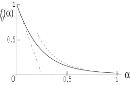
Figure 3: The function $f_{0}(\alpha)=U_{L}(\alpha)/U_{L}(0)$ for a short channel. Its asymptotic limits valid for small $\alpha$ (Eq. (12)) and large $\alpha$ (Eq. (14)) are shown by dash-dotted and dashed lines.

Now we formulate our results starting from a short channel, where electric field lines do not escape from the channel, $L<\xi$. At $\alpha\ll 1$ all ions form compact pairs and the effect of interactions between the pairs is small. Nevertheless, there is a linear in $\alpha\ll 1$ correction to the activation barrier:

$$U_{L}(\alpha)=(1-4\alpha)\,U_{L}(0)\,,$$ (12)

where $U_{L}(0)$ is given by Eq. (2). Although the relative correction is small, it may have a profound influence on the resistance of the channel. Indeed, since $4\alpha U_{L}(0)/(k_{B}T)=nL$, according to Eq. (3):

$$R(\alpha\ll 1)\sim R(0)\exp\{-nL\},$$ (13)

where $nL=c\pi a^{2}L$ is the number of ions in the volume of the channel in the bulk solution (not the actual number of ions in the channel). At $nL\gg 1$, the resistance is exponentially decreased in comparison with the zero concentration limit.

In the large $c$ limit, when $\alpha>1$, one may expect that the overlap of thermal pairs leads to the deconfinement transition at some critical concentration, $\alpha_{c}\simeq 1$. We show that such transition does not occur. Instead, the barrier proportional to the channel’s length exists at any concentration of the salt. Its magnitude, however, is exponentially suppressed at high salt concentration, i.e. for $\alpha\gg 1$:

$$U_{L}(\alpha)=2^{\,7}\pi^{-1/2}\alpha^{3/4}\exp\left\{-8\sqrt{\alpha}\right\}U_{L}(0)\,.$$ (14)

Thus the channel is always an insulator (one may call it a superinsulator, since $\ln R\propto L$, rather than $R\propto L$ as is the case for Ohmic resistors). The $\alpha$ dependence in Eq. (14) is similar to that obtained in Ref. Schultz for the inverse effective dielectric constant.

We plot numerically computed function $f_{0}(\alpha)\equiv U_{L}(\alpha)/U_{L}(0)$ along with its two asymptotic Eqs. (12) and (14) in Fig. 3. It is easy to verify that $f_{0}(\alpha)$ can be fitted by $f_{0}(\alpha)\approx\exp(-4\alpha)$ (not shown) within the accuracy of $10\%$ in the range $0<\alpha<0.94$, where $f_{0}(\alpha)$ decreases almost 50 times.

We turn now to the results for longer channels. The short channel results, outlined above, are valid for $L\leq L_{c}$, where $L_{c}=L_{c}(\alpha)$ is a certain threshold length. At $\alpha\ll 1$ we show that $L_{c}=\pi\sqrt{2\alpha}\,\xi$, so the correction term in Eq. (12) is valid for smaller channel’s length. At $L\gg L_{c}$ the barrier saturates at the value

$$U_{\infty}(\alpha)=(1-4\alpha^{2}\ln(1/\alpha))\,U_{\infty}(0)\,,$$ (15)

where $U_{\infty}(0)$ is given by Eqs. (7), (8).

In the $\alpha\gg 1$ limit, we obtain the exponentially large threshold length $L_{c}(\alpha)\sim\xi\exp\left\{4\sqrt{\alpha}\right\}$. Consequently, Eq. (14) is only valid as long as $L\leq L_{c}(\alpha)$. For even longer channels, $L\gg L_{c}(\alpha)$, we obtain:

$$U_{\infty}(\alpha)=2^{\,5}\pi^{-5/4}\alpha^{3/8}\exp\left\{-4\sqrt{\alpha}\right\}U_{\infty}(0).$$ (16)

Fig. 4 shows the ratio $f_{\infty}(\alpha)\equiv U_{\infty}(\alpha)/U_{\infty}(0)$ in the infinite channel along with that in the short one. We also calculated $f_{L}(\alpha)\equiv U_{L}(\alpha)/U_{L}(0)$ for several different ratios of $L/\xi$ and plotted these results in Fig. 4.

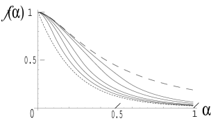
Figure 4: Effect of screening by salt for channels of different lengths. Ratios $U_{L}(\alpha)/U_{L}(0)$ as functions of $\alpha$ are plotted by the dashed line for the infinite channel ($f_{\infty}(\alpha)$) and by the dotted line for the short channel ($f_{0}(\alpha)$). Full lines represent the channels with (from top to bottom) $L/\xi=4,3,2,1.5,1$.

For the narrow channels, $a\lesssim l_{B}$, all the results, mentioned above, are still valid, provided that the dimensionless concentration $\alpha$ is substituted by the renormalized concentration $\alpha_{eff}$. The latter is defined and evaluated in section VI.

Above we have discussed the results pertinent to the exponential activation term in the linear resistance. The pre–exponential factor is discussed in section VII. We have also considered the exponential suppression of the differential resistance at large applied voltage, $V$. For the short channel we obtain the suppression of the activation barrier:

$$R(V)\sim\exp\left\{\frac{U_{L}(\alpha)-eV/2}{k_{B}T}\right\}\ ,$$ (17)

where the applied voltage $eV\leq 2U_{L}(\alpha)$. For a long channel where $L\gg L_{c}(\alpha)$, Eq. (17) (with $U_{L}\to U_{\infty}$) is valid as long as $eV<e^{2}/(\kappa_{2}L)$. In the opposite limit, $e^{2}/(\kappa_{2}L)<eV\leq 2U_{\infty}(\alpha)$, the long–range nature of the 3d Coulomb interaction through the dielectric media with $\kappa_{2}$ is important. It leads to the replacement of Eq. (17) by the Frenkel-Poole law Frenkel

$$R(V)\sim\exp\left\{\frac{U_{\infty}(\alpha)-(e^{3}V/L\kappa_{2})^{1/2}}{k_{B}T}\right\}\ .$$ (18)

In the next section we present simple qualitative derivations of the above results.

III Qualitative consideration

III.1 Concept of the boundary charges

Consider a relatively short channel where all field lines stay inside the channel (Fig. 1a). If the average distance between the ions is larger than $a$ each ion may be characterized by a single coordinate $x\in[-L/2,L/2]$ along the axis of the channel. We deal, thus, with the 1d plasma interacting through the one-dimensional Coulomb potential. Each ion is equivalent to a charged plane perpendicular to the $x$–axis with the charge density $\pm E_{0}/2\pi$. As discussed in the Introduction, a single negative ion in the middle of a channel has the self–energy $U_{L}(0)$. Half of its electric field exits to the right and half to the left. One may say that there are image boundary charges $q=1/2$ and $q^{\prime}=1/2$ on the left and right boundaries of the channel correspondingly (hereafter all image charges are measured in units of $e$). One can imagine that these charges are provided by the well conducting bulk plasma in the reservoirs.

The concept of the boundary charges, which are not supposed to be integer is central for the present work. Let us demonstrate the usefulness of the boundary charges by a simple example of the ion’s energy as function of its coordinate $x$. If the boundary charge at $x=-L/2$ is $0<q<1$, then the boundary charge at $x=L/2$ is $q^{\prime}=1-q$. Electric fields to the left and right of the test charge is $2qE_{0}$ and $2(1-q)E_{0}$, so that the energy of electric field $U(x;q)=(\kappa_{1}/2)E_{0}^{2}a^{2}[q^{2}(x+L/2)+(1-q)^{2}(L/2-x)]$. Optimizing this energy with respect to $q$, we find $q=1/2-x/L$ and for the energy as a function $x$ we arrive at

$$U(x)\!=\!{\kappa_{1}E_{0}^{2}a^{\,2}\over 2}\left({L\over 4}-{x^{2}\over L}\right)\!=\!\left(1-\left({2x\over L}\right)^{2}\right)\,U_{L}(0)\,.$$ (19)

This gives the parabolic barrier with the maximum value $U_{L}(0)$ in the middle of the channel (see Fig. 1a). The maximal barrier corresponds to $q=q^{\prime}=1/2$.

In a similar manner one may consider a pair of a negative ion with the coordinate $x_{1}$ and a positive ion with the coordinate $x_{2}$ inside the channel. They induce two boundary charges $q$ and $q^{\prime}=-q$. Writing the interaction energy of these four charges, one finds that it reaches its optimal value, given by $U(x_{1},x_{2})=4(|x_{12}|/L-x_{12}^{2}/L^{2})\,U_{L}(0)$, at $q=x_{12}/L$, where $x_{12}\equiv x_{1}-x_{2}$. At small separation, $|x_{12}|\ll L$ the ions attract each other with the string potential $eE_{0}|x_{1}-x_{2}|$ so that typical distance between them is $x_{T}$. Such a pair can contribute to the charge transport only if the positive and negative ions separate and move to the opposite ends of the channel. Remarkably, the energy barrier they have to overcome is given by $U_{L}(0)$. It is exactly the same as for the single ion. The maximum is reached when $|x_{12}|=L/2$, while $q=-q^{\prime}=1/2$.

One can repeat this calculation for an arbitrary number of pairs inside the channel. One can see that the maximum energy state, the system goes through to contribute to the charge transport, is always reached when $q=\pm 1/2$ and always has energy $U_{L}(0)$. We shall refer to such a state with the half-integer boundary charge as the collective saddle point configuration. Fig. 5 illustrates how the channel with three originally compact pairs oriented along the external electric field transfers a unit charge. It starts from the state with $q=-q^{\prime}\approx 0$, goes to the top of the barrier with $q=-q^{\prime}=1/2$ and ends up again in the state of compact pairs with $q=-q^{\prime}\approx 1$. The net result of such a process is a transfer of the unit charge across the channel.

Figure 5: Three consecutive states of the channel with three pairs. (a) Compact pairs with $q=-q^{\prime}\approx 0$, (b) the saddle point state with $q=-q^{\prime}=1/2$, (c) Compact pairs with $q=-q^{\prime}\approx 1$. Other saddle points may be obtained e.g. by moving the two same sign ions away from each other.

From the fact that the energy needed to transfer the charge is completely independent of the ion concentration one may tend to conclude that the same is true regarding the activation barrier. Such a conclusion is premature, however. Indeed, the activation barrier is given by the maximum of the free energy and thus includes the (negative) entropy contribution. As we explain below, the collective saddle point configuration possesses a huge degeneracy and thus has a rather large entropy. This entropy reduces the activation barrier down to Eq. (12).

For a more quantitative consideration one needs to discuss the exchange of ions between the bulk reservoirs and the channel. Although the concentration of single ions in the channel is strongly depleted, compact neutral pairs enter the channel freely. Thus, typically there are many interacting pairs of ions inside the channel. We have to discuss separately their equilibrium (minimum energy) state and their collective saddle point (barrier) state when they contribute to the transport. It is convenient to distinguish the range of relatively low concentrations $c$, when $\alpha\ll 1$, and the range of high concentrations, $\alpha>1$. The concept of the boundary charges, introduced above, is helpful in both cases.

III.2 Short channel at low concentration of salt

In this section we consider the case of low concentration of ions in the bulk salt solution, such that $\alpha\ll 1$. A typical concentration of pairs inside the channel is even lower: $n_{p}=2n\alpha\ll n$. To transfer the charge across the channel the plasma must go trough the collective saddle point state. Such saddle point is characterized by the half–integer boundary charge, say $q=1/2;\,q^{\prime}=-1/2$. Half–integer boundary charges apply the external electric field $E_{0}$ across the channel. All dipoles of compact pairs turn in the direction of the field, so that positive and negative ions alternate. One can see now that inside each pair the electric field changes its sign and turns to $-E_{0}$ (recall the analogy with the uniformly charged planes, producing field $E_{0}$ in both directions). As a result, at the points where charges are located the electric field switches between $E_{0}$ and $-E_{0}$. The electrostatic energy of the channel is still equal to $U_{L}(0)$ and does not depend on the positions of the charges. This makes the charges free (as long as they are ordered in the alternating sequence) from being connected into the compact pairs. We shall call such peculiar state – the ordered free plasma (OFP).

Since in the OFP state the individual charges are free to enter the channel, one expects that the concentration of free charges (rather than the much lower concentration of the compact pairs) is the same in the channel and in the bulk. (Due to the restriction of alternation the actual concentration in the channel happens to be half of the one in the bulk.) One may say that in the OFP state ($q=1/2;\,q^{\prime}=-1/2$) the gas of the free ions in the bulk expands into the channel. This leads to the growth of the system’s entropy and thus reduction of the activation barrier.

In order to calculate the entropy gain $\Delta S$ of the OFP state we assume that from the total number of ions, $2N$, some $2\Delta N$ enter into the channel’s volume $\Delta V=\pi a^{\,2}L$. The rest $2N-2\Delta N$ ions stay in the bulk volume $V$. In the bulk $N-\Delta N$ positive ions and $N-\Delta N$ negative ones produce additive contributions to the entropy. In the channel, however, the gas is ordered so that ions of different signs alternate and cannot exchange their positions. Therefore, the entropy is the same as that of $2\Delta N$ identical ions. Thus, the total entropy of the system is:

$${S\over k_{B}}=2(N-\Delta N)\ln\frac{eV/l_{0}^{3}}{N-\Delta N}+2\Delta N\ln\frac{e\Delta V}{2\Delta Nl_{0}^{3}}.$$ (20)

where $l_{0}^{3}$ is the normalization volume. The optimal value of $\Delta N$ maximizing $S$ is

$$\Delta N=\frac{1}{2}\,\frac{\Delta V}{V}\,N={nL\over 2}$$ (21)

and thus the entropy gain is:

$$\Delta S=k_{B}nL\,.$$ (22)

Recalling that the free energy at the collective saddle point is $U_{L}(\alpha)=U_{L}(0)-T\Delta S$, we arrive at Eq. (12). In this derivation we have neglected entropy change of the equilibrium state compared to $\Delta S$, because $n_{p}\ll n$. This simplification is equivalent to omitting corrections which are of the order of $\alpha^{2}$ in Eq. (12). This calculation is justified as long as $\Delta N\gg 1$.

III.3 Short channel at high concentration of salt

At high concentration of ions in the channel when $\alpha=nx_{T}>1$ the thermal pairs overlap. Thus, one may expect that the ions screen each other and become essentially free. If this is the case, the concentration of ions inside the channel equals to that outside, i.e. the 1d concentration is equal to $n$. It is natural to approach such a dense plasma with the mean-field Debye-Hückel approximation. Recalling the analogy with the charged planes, one needs to calculate the screening of a plane by other planes. This is exactly what happens when 3d plasma screens a plane. As a result, the electric field of a unit charge at a distance $x$ is expected to be:

$$E(x)=E_{0}\,e^{-|x|/x_{D}}\,,$$ (23)

where the Debye length, $x_{D}$, is given by the standard expression:

$$x_{D}=\left({k_{B}T\over 8\pi ce^{2}}\right)^{1/2}=a\left({k_{B}T\over 8ne^{2}}\right)^{1/2}.$$ (24)

In terms of $\alpha$ one has: $x_{D}\sim n^{-1}\alpha^{1/2}\sim x_{T}\alpha^{-1/2}$, so that $n^{-1}<x_{D}<x_{T}$ for $\alpha\gg 1$.

The interaction energy of the system may be written as

$$W=\frac{\kappa_{1}a^{\,2}L}{8}\!\int\limits_{-\infty}^{\infty}\!\!dE\,E^{2}\,{\cal P}(E)\,,$$ (25)

where ${\cal P}(E)$ is the distribution function of the random electric field in the channel. For $\alpha\gg 1$ it is Gaussian:

$${\cal P}(E)=(2\pi\langle E^{2}\rangle)^{-1/2}\exp\left[-E^{2}/2\langle E^{2}\rangle\right]$$ (26)

with the mean square average value $\langle E^{2}\rangle=4nx_{D}E_{0}^{2}=W/(\pi a^{2}L)$. Indeed, fluctuations of the electric field are created by the fluctuations of number of positive and negative charges in two adjacent segments of the channel of the length $x_{D}$ each. A typical fluctuation has opposite charges of the order of $Q\sim(nx_{D})^{1/2}$, which interaction energy is $k_{B}T$. Thus, it creates the electric field of the order of $2QE_{0}=2(nx_{D})^{1/2}E_{0}$.

As was discussed above, the activation barrier is associated with the (free) energy difference between the state with half–integer and integer boundary charges. According to the Debye-Hückel theory any boundary charge is completely screened at the Debye length, $x_{D}$, and thus is a local perturbation. Then the aforementioned energy difference is not an extensive quantity and is proportional to $x_{D}$ rather than the channel length, $L$, as was the case in the low density limit. Such a qualitative change in the scaling of the activation barrier may occur only as a result of a phase transition at some $\alpha_{c}\simeq 1$, where the $L$–dependent part of the activation barrier vanishes. It is well–known, however, that the thermodynamics of 1d Coulomb gas, being well described by the Debye-Hückel theory, does not exhibit any phase transitions Lenard ; Edwards ; Schultz . Thus, one either has to explain how the Debye-Hückel thermodynamics may be consistent with the $L$–dependent activation barrier, or find a phase transition in the activation barrier which is not seen in the equilibrium thermodynamics. We show below how the former of these two alternatives works. There is no phase transition in the activation barrier. Instead, the $L$-dependent activation energy decreases exponentially with increasing $\alpha$ at $\alpha>1$.

The crucial point is that the Debye–Hückel approximation misses the discreteness of charge. Since the charges are discrete, the electric field along the channel may change only in the steps of $\pm 2E_{0}$, at the points where the charges are located. Therefore at any point in the channel, having the boundary charges $q$ and $q^{\prime}=-q$, the electric field may be equal to $2E_{0}(q+M)$. Here $M$ is an integer, given by the total charge to the left of the point in question. In this manner the information about the boundary charges “propagates” through the entire channel (in an apparent contradiction to the Debye–Hückel prediction, Eq. (23)).

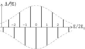
Figure 6: The function $\Delta{\cal P}(E)$ is the difference of discrete distribution functions of electric field for $q=1/2$ and $q=0$, which are made of set of $\delta$–functions weighted with the envelope function ${\cal P}(E)$ given in Eq. (26).

Let us show now that this “quantization” of the electric field leads to the activation barrier proportional to $L$, though with the exponentially small coefficient. To this end we employ the distribution function of the electric fields, Eq. (26), as a weighting factor for the quantized values of the electric field $2E_{0}(q+M)$. For example, at $q=0$ we sum over integers, while at $q=1/2$ the sum is over half-integers. The transport barrier $U_{L}(\alpha)=W(1/2)-W(0)$ is the difference between these two sums, or in other words:

$$U_{L}(\alpha)=\frac{\kappa_{1}a^{\,2}L}{8}\int\limits_{-\infty}^{\infty}\!\!E^{2}\,\Delta{\cal P}(E)dE,$$ (27)

where $\Delta{\cal P}$ is the difference of discrete distribution functions for $q=1/2$ and $q=0$ illustrated in Fig. 6. It is clear that $U_{L}(\alpha)$ is exponentially small. Performing summation over integer $M$ (instead of the integration, as in Eq. (25)) with the help of the Poisson summation formula, one finds the activation energy:

$$U_{L}(\alpha)=-\frac{\kappa_{1}a^{\,2}L}{8}\int\limits_{-\infty}^{\infty}\!\!dE\,E^{2}\,{\cal P}(E)\cos(\pi E/E_{0})\,.$$ (28)

As a result, one finds for the activation barrier $U_{L}(\alpha)\sim U_{L}\exp\{-\pi^{2}\sqrt{\alpha}\}$. Similarly to the dilute case the activation barrier is proportional to the channel’s length. Upon increasing the salt concentration the barrier monotonously decreases without undergoing the phase transition. Comparing the exponent with the exact result, Eq. (14), one notices that the coefficient is slightly overestimated ($\pi^{2}$ instead of $8$). The reason is that the fields $E$, contributing to the integral in Eq. (28), correspond to the charge of an optimal fluctuation of the order $Q\approx enx_{D}$. Therefore both assumptions of the applicability of the Gaussian distribution and the theory of the Debye-Hückel linear screening to the optimal charge fluctuations are only marginally correct. The quantitative theory of the next section goes beyond these limitations. Unlike the activation barrier, the thermodynamics is very weakly affected by the “quantization” and is given by the Debye-Hückel theory Lenard ; Edwards (up to exponentially small corrections).

III.4 Long channel

In the previous sections we dealt only with a short channel, where the electric field does not escape from the channel to the media with the small dielectric constant $\kappa_{2}$. For finite $\alpha$ the energy of the electric field is decreased due to the screening by other ions. One may interpret this decrease of the activation barrier as an enhancement of the dielectric constant: $\kappa_{1}\to\kappa_{1}(\alpha)\equiv\kappa_{1}/f_{0}(\alpha)$. Indeed, from Eq. (2), one may write $U_{L}(\alpha)=e^{2}L/(2\kappa_{1}(\alpha)a^{\,2})=f_{0}(\alpha)U_{L}(0)$.

Employing the concept of the concentration–dependent dielectric constant, one may formulate the results for the self-energy of an ion in the long channel. Indeed, both the characteristic length of the electric field decay, $\xi\to\xi(\alpha)$, and the self–energy barrier, $U_{\infty}(0)\to U_{\infty}(\alpha)$, are functions of the dielectric constant $\kappa_{1}$ (see Eqs. (7), (8)), which depends now on the concentration: $\kappa_{1}\to\kappa_{1}(\alpha)$. The approximate solution of Eq. (7) for $\xi(\alpha)$ is:

$$\xi(\alpha)\approx a\,\sqrt{\kappa_{1}(\alpha)\over\kappa_{2}}\,\ln^{1/2}\left({\kappa_{1}(\alpha)\over\kappa_{2}}\right)\,,$$ (29)

$$U_{\infty}(\alpha)=\frac{e^{2}}{a}\,\,\frac{\ln^{1/2}(\kappa_{1}(\alpha)/\kappa_{2})}{\sqrt{\kappa_{1}(\alpha)\kappa_{2}}}.$$ (30)

Since according to Eq. (14), $f_{0}(\alpha)\sim e^{-8\sqrt{\alpha}}$ for $\alpha>1$, one finds $\kappa_{1}(\alpha)\sim\kappa_{1}e^{8\sqrt{\alpha}}$. According to Eqs. (29), (30) the decay length of the field $\xi(\alpha)\sim e^{4\sqrt{\alpha}}$ grows exponentially and the self–energy barrier is $U_{\infty}(\alpha)\sim e^{-4\sqrt{\alpha}}$, cf Eq. (16).

For $\alpha\ll 1$ one must take into account deviations of $E(x)$ from $E_{0}$, cf. Eq. (6). As was discussed in section III.2, Eq. (12) is based on the fact that the field $E_{0}$ makes the pairs of positive and negative ions free. A somewhat smaller field $E(x)$ leaves most of the pairs bound. However, even bound pairs contribute to the entropy growth. Let us consider a point charge in the middle of the channel with the field decaying according to Eq. (6). It is easy to see that the average arm of pairs grows for the dipoles oriented along the direction of the electric field $E(x)$. For the oppositely oriented pairs the arm shrinks. As a result, the average pair length becomes $2x_{T}(x)=2x_{T}E_{0}^{2}/[E_{0}^{2}-E^{2}(x)]$ and for the local concentration of pairs instead of Eq. (10) we find: $n_{p}(x)=2n^{2}x_{T}(x)=n_{p}E_{0}^{2}/[E_{0}^{2}-E^{2}(x)]$. This estimate is valid for $|x|>\alpha\xi$, while at smaller distances $n_{p}\approx n/2$. Thus the total number of pairs, $N_{p}$, brought into the channel by the central charge may be estimated as:

$$\Delta N=2\int\limits_{\alpha\xi}^{L}[n_{p}(x)-n_{p}]dx=2n\xi\alpha\ln(1/\alpha),$$ (31)

The new pairs add the entropic term $-k_{B}T\Delta N$ to the free energy of the channel with the fixed central charge. This entropic contribution leads to the suppression of the transport barrier given by Eq. (15).

III.5 Non-ohmic transport of the channel at large voltage

Until now we dealt with the ohmic transport limited by small voltages $eV\ll k_{B}T$. Let us consider the effect of a finite voltage on the differential resistance in the opposite case, $eV>k_{B}T$. We start from a short channel. As was discussed above, the top of the transport barrier corresponds to the boundary charges $\pm 1/2$. These charges are provided by the potential source which makes the work $eV/2$. Thus, the conductance barrier becomes lower by this energy and we arrive at Eq. (17).

In the long channel the electric field lines of a moving charge leave the channel, go to the low dielectric constant media and eventually return to the water solution far from the channel. Thus, each moving charge creates the two opposite sign images in the two water–filled semi–spaces. These images are similar to the boundary charges. Attraction to each of them follows the three dimensional Coulomb law. For example, a charge with the coordinate $x$ close to $-L/2$ is attracted to the image with the energy $-e^{2}/[4\kappa_{2}(L/2+x)]$, if $L/2+x\gg\xi$. The sum of the attraction energies to both water semi-spaces has maximum at $x=0$. Thus, the top of the barrier corresponds to the charge located at the center. In this position the image charges are equal $q=q^{\prime}=1/2$. If the applied electric field $V/L$ is smaller than the field of each image in the center, $2e/(\kappa_{2}L^{2})$, the field only weakly affects position of the saddle point. At such conditions the voltage only reduces the barrier by $eV/2$. Thus, for a long channel one gets similarly to Eq. (17):

$$R(V)\sim\exp\left\{\frac{U_{\infty}(\alpha)-eV/2}{k_{B}T}\right\}\,$$ (32)

On the other hand, if $V/L\gg 2e/(\kappa_{2}L^{2})$ the shape of the barrier changes drastically. It looses the symmetry around $x=0$. The saddle point moves to the distance $l\ll L/2$ from the left border. The length $l$ is determined by the maximum of the sum of the attractive Coulomb potential of the charge to the left image and the linear potential of the uniform electric field $V/L$. This maximum is located at the distance $l=(eL/4\kappa_{2}V)^{1/2}$. As a result, the barrier is reduced by $2eVl/L=(e^{3}V/\kappa_{2}L)^{1/2}$, thus we arrive at Eq. (18). This result was first derived by Frenkel Frenkel for the field–induced ionization of Coulomb impurities in semiconductors.

The longer the channel, the smaller is the range of applicability of Eq. (32) and the larger is the range of applicability of Eq. (18). Notice that the applied voltage $V$ does not interfere with the effect of the salt on the barrier height. In the Eq. (17), Eq. (32) and Eq. (18) the concentration–dependent height of the barrier determines only the voltage at which the activation exponent is of order one. Equations (17), (32) and (18) are valid only at smaller voltages.

IV Thermodynamics of the short channel

IV.1 Partition function

In this section we focus on a relatively short channel, such that the electric field lines do not escape to the media with the small dielectric constant. The calculation of the partition function is similar to that in Ref. Edwards . We briefly reproduce it here to focus on the role of the boundary charges and to generalize it later to the short channel case. The interaction energy of plasma consisting of $N$ positive and $N^{\prime}$ negative charges is given by

$$U={1\over 2}\sum\limits_{i,j=1}^{N+N^{\prime}}\sigma_{i}\sigma_{j}\Phi(x_{i}-x_{j})\,,$$ (33)

where $\sigma_{j}=1$ for $j=1,\ldots N$ and $\sigma_{j}=-1$ for $j=N+1,\ldots N+N^{\prime}$. The interactions are mediated through the 1d Coulomb potential:

$$\Phi(x)=\Phi(0)-eE_{0}|x|$$ (34)

Here $\Phi(0)$ is an artificial constant (twice of the ion’s self–energy) which is used to impose charge neutrality by taking $\Phi(0)\to\infty$ limit. To this end the diagonal terms, representing the self-energy of the charges are included in Eq. (33).

Following discussion of Section III.1, one also introduces two boundary (in general non-integer) charges $q$ and $q^{\prime}$ at the end points of the channel $x=\mp L/2$. With these two charges included the total energy takes the form:

$$U(q,q^{\prime})={1\over 2}\int\!\!\!\!\!\!\int\limits_{-L/2}^{L/2}\!\!dxdx^{\prime}\rho(x)\Phi(x-x^{\prime})\rho(x^{\prime})\,,$$ (35)

where the charge density is defined as

$$\rho(x)\equiv\!\!\sum\limits_{j=1}^{N+N^{\prime}}\!\!\sigma_{j}\delta(x-x_{j})+q\delta(x+L/2)+q^{\prime}\delta(x-L/2)\,.$$ (36)

We are interested in the grand-canonical partition function of the gas defined as

$$Z_{L}(q,q^{\prime})=\sum\limits_{N,N^{\prime}=0}^{\infty}e^{\mu(N+N^{\prime})/(k_{B}T)}{1\over N!N^{\prime}!}$$ (37)

$$\times\prod\limits_{j=1}^{N+N^{\prime}}\left({\pi a^{\,2}\over l_{0}^{2}}\int\limits_{-L/2}^{L/2}{dx_{j}\over l_{0}}\right)e^{-{1\over k_{B}T}U(q,q^{\prime})}\,,$$

where $\mu$ is the chemical potential of the charges (the same for pluses and minuses) and $l_{0}$ is a microscopic scale related to the bulk salt concentration as $c=e^{\mu/k_{B}T}/l_{0}^{3}$. Factor $\pi a^{2}/l_{0}^{2}$ originates from the integrations over transverse coordinates. Since we have in mind the viscous dynamics of the ions, rather than the inertial one, the kinetic energy is not included in the partition function.

Formally any configuration of $N$ pluses and $N^{\prime}$ minuses is allowed in this expression. One expects, though, that only neutral configurations with $N-N^{\prime}+q+q^{\prime}=0$ provide non–zero contributions due to the presence of the large self–energy, $\Phi(0)$. As a result, one expects that $Z_{L}(q,q^{\prime})\sim\delta_{q^{\prime},m-q}$, where $m=N^{\prime}-N$ is an integer number. We shall see later that this is indeed the case.

To proceed with the evaluation of $Z_{L}(q,q^{\prime})$ we introduce the resolution of unity written in the following way:

$$1 = \int\!\!{\cal D}\!\rho(x)\,\,\delta\!\!\left(\rho(x)-\sum\limits_{j=1}^{N+N^{\prime}}\sigma_{j}\delta(x-x_{j})-q\delta(x+L/2)-q^{\prime}\delta(x-L/2)\right)$$

$$= \int\!\!{\cal D}\!\rho(x)\int\!\!{\cal D}\theta(x)\,\,\exp\left\{\,-i\!\!\!\int\limits_{-L/2}^{L/2}\!dx\,\theta(x)\left(\rho(x)-\sum\limits_{j=1}^{N+N^{\prime}}\sigma_{j}\delta(x-x_{j})-q\delta(x+L/2)-q^{\prime}\delta(x-L/2)\right)\right\}$$

$$= \int\!\!\!\int{\cal D}\!\rho(x){\cal D}\theta(x)\,\,\exp\left\{\,-i\left(\int\limits_{-L/2}^{L/2}\!dx\,\theta(x)\rho(x)-\sum\limits_{j=1}^{N+N^{\prime}}\sigma_{j}\theta(x_{j})-q\theta(-L/2)-q^{\prime}\theta(L/2)\right)\right\}~{}.$$

Substituting this identity into the expression for the partition function, one finds:

$$Z(q,q^{\prime})= \int\!\!\!\!\int\limits_{-\infty}^{\infty}\frac{d\theta_{i}d\theta_{f}}{4\pi^{2}}\,\,e^{iq\theta_{i}+iq^{\prime}\theta_{f}}\int\!\!\!\int{\cal D}\!\rho(x){\cal D}\theta(x)\,\exp\left\{-{1\over 2k_{B}T}\int\!\!\!\int\limits_{-L/2}^{L/2}\!\!dxdx^{\prime}\rho(x)\Phi(x-x^{\prime})\rho(x^{\prime})-i\int\limits_{0}^{L}\!dx\,\theta(x)\rho(x)\right\}$$ (39)

$$\times\sum\limits_{N=0}^{\infty}{1\over N!}\,e^{\mu N/(k_{B}T)}\left({\pi a^{\,2}\over l_{0}^{3}}\int\!\!dx\,e^{i\theta(x)}\right)^{N}\times\sum\limits_{N^{\prime}=0}^{\infty}{1\over N^{\prime}!}\,e^{\mu N^{\prime}/(k_{B}T)}\left({\pi a^{\,2}\over l_{0}^{3}}\int\!\!dx\,e^{\,-i\theta(x)}\right)^{N^{\prime}}$$

$$= \int\!\!\!\!\int\limits_{-\infty}^{\infty}\frac{d\theta_{i}d\theta_{f}}{4\pi^{2}}\,\,e^{iq\theta_{i}+iq^{\prime}\theta_{f}}\int\!\!{\cal D}\theta(x)\,\,\exp\left\{-{k_{B}T\over 2}\int\!\!\!\int\limits_{-L/2}^{L/2}\!\!dxdx^{\prime}\theta(x)\Phi^{-1}(x-x^{\prime})\theta(x^{\prime})+2\pi a^{\,2}c\int\limits_{-L/2}^{L/2}\!dx\cos\theta(x)\right\}\,.$$

The integral over $\theta(x)$ runs over all functions with the boundary conditions $\theta(-L/2)=\theta_{i}$ and $\theta(L/2)=\theta_{f}$. It is straightforward to verify that $\Phi^{-1}$ operator is given by $\Phi^{-1}(x-x^{\prime})=-(2eE_{0})^{-1}\delta(x-x^{\prime})\partial^{2}_{x}$. As a result, the functional integral on the r.h.s. of the last expression takes the form

$$G_{L}(\theta_{i},\theta_{f})\equiv\int\!\!{\cal D}\theta(x)\,\,e^{-{x_{T}\over 2}\!\int\!\!dx\left[{1\over 2}(\partial_{x}\theta)^{2}-{4\alpha\over x_{T}^{2}}\cos\theta(x)\right]}\,,$$ (40)

where $x_{T}$ and $\alpha$ are given by Eqs. (4) and (11).

Expression (40) represents the “quantum mechanical” probability to propagate from the point $\theta_{i}$ to the point $\theta_{f}$ during the (imaginary) “time” $L$. The corresponding “Schrödinger equation” for the “wave-function” $\Psi=\Psi(\theta,x)$ has the form:

$$-{1\over 2}\frac{\partial^{2}\Psi}{\partial\theta^{2}}-\alpha\cos\theta\,\,\Psi=-{x_{T}\over 2}{\partial\Psi\over\partial x}\,.$$ (41)

One may look for the eigenfunctions of this equation: $\Psi_{k}(\theta,x)=\Psi_{k}(\theta)\exp\{-2\,\epsilon_{k}x/x_{T}\}\,$, labelled by a quantum number $k$. The corresponding “Schrödinger equation” for the stationary eigenfunctions has the form:

$$-{1\over 2}\frac{\partial^{2}\Psi_{k}(\theta)}{\partial\theta^{2}}-\alpha\cos\theta\,\,\Psi_{k}(\theta)=\epsilon_{k}\Psi_{k}(\theta)\,,$$ (42)

where $\epsilon_{k}$ is the energy. In terms of the stationary eigenfunctions the propagator takes the form:

$$G_{L}(\theta_{i},\theta_{f})=\sum\limits_{k}\Psi_{k}(\theta_{i})\bar{\Psi}_{k}(\theta_{f})\,e^{-2\epsilon_{k}L/x_{T}}\,.$$ (43)

Finally, the partition function, Eq. (39), is nothing but the propagator in the momentum representation and thus may be written as:

$$Z_{L}(q,q^{\prime})=G_{L}(q,-q^{\prime})=\sum\limits_{k}\Psi_{k}(q)\bar{\Psi}_{k}(-q^{\prime})\,e^{-2\epsilon_{k}L/x_{T}}\,,$$ (44)

where $\Psi_{k}(q)\equiv\int d\theta/(2\pi)\Psi_{k}(\theta)\exp\{i\theta q\}$. Relation between the thermodynamics of the 1d Coulomb gas and the Mathieu equation (42) was realized long ago by Lenard Lenard . He was interested, however, only in the equilibrium thermodynamics, rather than the transport characteristics.

IV.2 Green function

One can employ now the well-known results for the Schrödinger equation in the periodic potential, Eq. (42), to find the propagator, $G_{x}(q,\tilde{q})$. The wave-functions are given by the Bloch-waves:

$$\Psi_{k}^{(j)}(\theta)=e^{-ik\theta}u_{k}^{(j)}(\theta)=e^{-ik\theta}\sum\limits_{m=-\infty}^{\infty}u_{k,m}^{(j)}e^{-im\theta}\,,$$ (45)

where $|k|<1/2$ is the quasimomentum and $u_{k}^{(j)}(\theta)$ is the period-$2\pi$ (Bloch) function in the $j$-th band. In the last expression one has expanded the Bloch function in the Fourier series. The Fourier transform of the eigenfunction with the quantum numbers $k,(j)$ is therefore given by

$$\Psi_{k}^{(j)}(q)=u_{k,m}^{(j)}\delta(q-k-m)\,,$$ (46)

where $m=q-k$ must be an integer, while $|k|<1/2$; i.e. $k=[q]$, where the square brackets denote the fractional part. We found, thus, that the propagator conserves momentum up to an integer $m$ (umklapp processes): $q=\tilde{q}+m$. This is a manifestation of the charge neutrality. The integer parts of $q$ and $q^{\prime}=-\tilde{q}$ may be arbitrary. Since the integer parts may be easily screened by attracting the corresponding number of counter-ions from the solution, they do not play an important role in the subsequent discussion. One finds then for the Green function:

$$G_{x}(q,\tilde{q})=\delta([q]-[\tilde{q}])\sum\limits_{j}u_{[q],m}^{(j)}\bar{u}_{[q],\tilde{m}}^{(j)}\,e^{-2\epsilon_{q}^{(j)}x/x_{T}}\,,$$ (47)

where we have used the fact that the band dispersion $\epsilon_{k}^{(j)}$ is a periodic function of the quasimomentum. The common fractional part of the boundary charges plays the role of the Bloch quasimomentum. It is important to notice that if $q$ is fixed, only the single state from each Bloch band contributes to the partition function.

For a sufficiently long channel, only the lowest Bloch band, $j=0$, should be retained in this expression, while the upper bands provide exponentially small corrections. Since the free energy is given by the logarithm of the propagator, one may also disregard $u_{q,m}^{(0)}$ factors. Indeed, the latter contribute to the free energy only a $L$–independent (boundary) term, which is relatively small if $L\gg x_{T}$. Therefore, the propagator may be approximated by:

$$G_{x}(q,\tilde{q})\approx\delta([q]-[\tilde{q}])\,e^{-2\epsilon_{q}^{(0)}x/x_{T}}\,,$$ (48)

where the $\epsilon_{q}^{(0)}(\alpha)$ is the dispersion relation of the lowest Bloch–Mathieu band. Finally, the extensive part of the free energy of the channel according to Eq. (44) is given by:

$$F_{L}(q)\equiv-k_{B}T\ln Z_{L}(q,q^{\prime})=k_{B}T\,\frac{2L}{x_{T}}\,\epsilon^{(0)}_{q}\,,$$ (49)

provided $[q^{\prime}]=-[q]$. The fact that the free energy is a periodic function of $q$ with the unit period reflects the perfect screening of the integer part of the boundary charge.

IV.3 Lowest Bloch band

Since the free energy is given by the dispersion relation $\epsilon_{q}^{(0)}(\alpha)$, let us discuss this function in more details. We concentrate on the first Brillouin zone: $|q|<1/2$.

In the extreme low concentration limit, $\alpha\to 0$, the dispersion relation is given by $\epsilon^{(0)}_{q}=q^{2}/2$. In the dilute limit, $\alpha\ll 1$, the cosine potential in Eq. (42) may be treated in the perturbation theory. Save for the points $q=\pm 1/2$, there are no first order corrections. The second order perturbation theory leads to:

$$\epsilon^{(0)}_{q}\approx{q^{2}\over 2}-\frac{\alpha^{2}}{1-4q^{2}}\,.$$ (50)

The divergency at $q=\pm 1/2$ signifies that the narrow interval around these two points, $|q\mp 1/2|\lesssim\alpha\ll 1$, requires a special treatment. Indeed, in the narrow region around $q=\pm 1/2$ points the energy gap opens up. Linearizing the bare spectrum $\,q^{2}/2\,$ in the vicinity of these points, one reduces the Schrödinger equation to the spectral problem for the $2\times 2$ matrix Hamiltonian:

$${1\over 2}\left(\begin{array}[]{cc}{1\over 4}+{\delta q}&{\alpha}\\ {\alpha}&{1\over 4}-{\delta q}\end{array}\right)\,,$$ (51)

where $\delta q\equiv 1/2\pm q$. Finding the spectrum, one obtains that the lowest Bloch band at $|\delta q|\lesssim\alpha$ takes the form:

$$\epsilon^{(0)}_{q}\approx{1\over 8}\left(1-4\sqrt{\alpha^{2}+\delta q^{2}}\right)\,.$$ (52)

At $q=\pm 1/2$ the energy reaches its maximum $\epsilon^{(0)}_{1/2}=(1-4\alpha)/8$.

In the high concentration limit, $\alpha>1$, the amplitude of the cosine potential is large. The band is narrow and is centered near the ground-state of an isolated (almost) parabolic potential well:

$$\epsilon_{q}^{(0)}\approx-\alpha+{1\over 2}\sqrt{\alpha}\,.$$ (53)

The momentum dispersion originates from the tunnelling between the adjacent wells. One may treat it in the tight–binding approximation and find for the dispersion relation:

$$\epsilon_{q}^{(0)}=-\alpha+{\sqrt{\alpha}\over 2}-2^{-4}f_{0}(\alpha)\cos(2\pi q)\,.$$ (54)

The band-width, $2^{-3}f_{0}(\alpha)$, may be calculated in the WKB approximation (for the numerical factor see Ref. AS, ):

$$2^{-3}f_{0}(\alpha)=2^{4}\pi^{-1/2}\alpha^{3/4}\exp\left\{-8\sqrt{\alpha}\,\right\}\,.$$ (55)

IV.4 Thermodynamics

One can employ now Eq. (49) to extract the thermodynamic characteristics of the 1d Coulomb plasma (see also Ref. Lenard, ). In particular, we are interested in the salt concentration inside the channel and the average interaction energy. The former is given by:

$$n_{p}=-{1\over 2L}{\partial F\over\partial\mu}=-{1\over 2L}{\partial F\over\partial\alpha}{\partial\alpha\over\partial\mu}=-n\,{\partial\epsilon_{q}^{(0)}(\alpha)\over\partial\alpha}\,,$$ (56)

while the interaction energy is:

$$W=-T^{2}{\partial\over\partial T}\left({F\over T}\right)=-2nLk_{B}T\alpha{\partial\over\partial\alpha}\left({\epsilon_{q}^{(0)}(\alpha)\over\alpha}\right)\,.$$ (57)

For low concentration, $\alpha\ll 1$, and $|q\mp 1/2|>\alpha$ the pair concentration is: $n_{p}(q)=2n\alpha/(1-4q^{2})$. This means that as long as $|q\mp 1/2|>\alpha$, the pair concentration inside the channel is low $n_{p}\ll n$. In terms of $n_{p}$ the free energy takes the simple form: $F(n_{p})=\mbox{const}-Ln_{p}k_{B}T$, corresponding to the ideal gas of dipole pairs. The interaction energy is given by $W=eE_{0}Lq^{2}+n_{p}Lk_{B}T$, showing that there is energy $k_{B}T$ per pair (in addition to the interaction energy of the boundary charges).

Consider now the narrow region around $q=\pm 1/2$ points, where $|q\pm 1/2|\lesssim\alpha$. Employing Eq. (52), one finds for the pair concentration: $n_{p}(1/2)=n/2\gg n_{p}(0)$. In fact, it is only half of the naive non–interacting estimate for the pair concentration inside the channel: $n$. This is the OFP state, where the ions are free to move as long as they are ordered in the alternating sequence. Indeed, for the free energy one finds $F(n_{p})=\mbox{const}-2Ln_{p}k_{B}T$, indicating an ideal gas of individual ions. For $q=1/2$ one has $W=eE_{0}L(1/2)^{2}$, meaning that the entire interaction energy comes from the boundary charges and not from the inside pairs. Notice that slightly away from the collective saddle point, $q=1/2$, the plasma in the channel is strongly non–ideal.

In the dense limit $\alpha>1$ the thermodynamic properties are almost independent from the boundary charges, $q$. Employing Eq. (53), one finds: $n_{p}=n-n/(4\sqrt{\alpha})$. The concentration in the channel is almost equal to the bulk concentration. For the interaction energy one finds $W=nLk_{B}T/(2\sqrt{\alpha})$ in exact agreement with the Debye-Hückel calculation, cf. Eq (25). Since the interaction energy per ion is much less than the temperature, the thermodynamics of the plasma is almost identical to that of the ideal gas of free ions Lenard . Despite of this, the plasma possesses a thermodynamically extensive ($\propto L$) activation barrier for the charge transport.

IV.5 Activation barrier

To calculate the activation barrier, one needs to find the free energy of the collective saddle point state. To this end we introduce an additional unit charge (say negative) at some point, $x_{0}$, inside the channel. Due to the perfect charge neutrality the system must respond by bringing two screening boundary charges: $q$ and $q^{\prime}=1-q$, where $q$ depends on $x_{0}$. An example of such dependence is discussed above, see Eq. (19). One can invert the logic and claim that by changing the boundary charge $q$ one changes the equilibrium position of the test charge, $x_{0}$. It is clear that by varying $q$ from zero to one, the negative charge is moved from $x_{0}=L/2$ to $x_{0}=-L/2$. The activation barrier for such process is determined by the maximum of the free energy as function of $q$. According to Eqs. (44), (48) and (49) the partition function is given by:

$$Z_{L}(q,1-q)=G_{L}(q,q-1)=e^{-2\epsilon^{(0)}_{q}L/x_{T}}\,.$$ (58)

Thus the free energy reaches the maximum at $q=1/2$, which corresponds to the test charge being in the middle of the channel. The minima are reached at $q=0$ and $q=1$, corresponding to the test charge being at $x_{0}=\pm L/2$.

Finally, the activation barrier is given by:

$$U_{L}(\alpha)=F_{L}(1/2)-F_{L}(0)=U_{L}(0)f_{0}(\alpha)\,,$$ (59)

where the bare barrier $U_{L}(0)$ is given by Eq. (2) and the universal function $f_{0}(\alpha)$ is proportional to the Bloch band-width:

$$f_{0}(\alpha)=8\left(\epsilon^{(0)}_{1/2}(\alpha)-\epsilon^{(0)}_{0}(\alpha)\right)\,.$$ (60)

This function is plotted in Fig. 3. The two limiting cases of low and high concentration, Eqs. (12) and (14), follow immediately from Eqs. (52) and (55), correspondingly.

V Long and intermediate channels

V.1 Partition function

In the long channel $L>\xi>x_{T}$, where the characteristic length $\xi$ is given by Eq. (7), the electric field lines escape to the media with the small dielectric constant, $\kappa_{2}$. As a result, the interaction potential gradually looses it 1d character and crosses over to the 3d Coulomb law $\Phi(x)\sim 1/(\kappa_{2}x)$. According to Eq. (6) in the large range of distances it has the form:

$$\Phi(x)=eE_{0}\xi\,e^{-|x|/\xi}\,.$$ (61)

Our previous consideration, c.f. Eq. (34), corresponds to the limit $\xi\to\infty$. Since $\Phi(0)=eE_{0}\xi\equiv 2U_{\infty}(0)$ (c.f. Eq. (8)) is now finite, there is no reason to expect the strict charge neutrality. It is straightforward to invert Eq. (61): $\Phi^{-1}(x-x^{\prime})=(2eE_{0})^{-1}\delta(x-x^{\prime})(\xi^{-2}-\partial^{2}_{x})$. Thus, one can repeat the mapping onto the quantum mechanics and arrive at the following Schrödinger equation for the wave-function $\Psi(\theta,x)$:

$$-{1\over 2}\frac{\partial^{2}\Psi}{\partial\theta^{2}}-\alpha\cos\theta\,\,\Psi+{1\over 2}\left({x_{T}\over 2\xi}\right)^{2}\theta^{2}\,\Psi=-{x_{T}\over 2}{\partial\Psi\over\partial x}\,.$$ (62)

As before, the grand–canonical partition function, $Z_{L}(q,q^{\prime})$, of the plasma with the fixed boundary charges is given by Eq. (44):

$$Z_{L}(q,q^{\prime})=G_{L}(q,-q^{\prime})=\sum\limits_{k}\Psi_{k}(q)\bar{\Psi}_{k}(-q^{\prime})\,e^{-2\epsilon_{k}L/x_{T}}\,.$$ (63)

This is nothing but the Green function of Eq. (62) in the momentum representation.

We shall show now that one may use the small parameter $x_{T}/(2\xi)\ll 1$ to find the Green function $G_{x}(q,\tilde{q})$ in the quasiclassical approximation. The results obtained this way are restricted to the concentration range $\alpha>\sqrt{x_{T}/\xi}$. For lower concentrations one may use the standard first order perturbation theory in $\alpha$ for Eq. (62). It leads to the linear in $\alpha$ correction to the activation barrier, which is bound to be smaller than $k_{B}T$ if $\alpha<\sqrt{x_{T}/\xi}$. By this reason we shall not discuss it here.

To proceed we rewrite the Schrödinger equation (62) in the basis of the Bloch waves, $\Psi_{k}^{(j)}(\theta)$, Eq. (45). This basis diagonalizes the first two terms on the l.h.s. of Eq. (62). The only non–diagonal term in this basis is the confinement potential proportional to $\theta^{2}$. In the Bloch basis it takes the form $-\delta_{k,k^{\prime}}[\delta^{j,j^{\prime}}\partial^{2}_{k}+2v^{j,j^{\prime}}_{1}(k)\partial_{k}+v^{j,j^{\prime}}_{2}(k)]$, where $v_{s}^{j,j^{\prime}}(k)=\sum_{m}\bar{u}_{k,m}^{(j)}\partial_{k}^{s}u_{k,m}^{(j^{\prime})}$ and $s=1,2$. Fortunately, one does not need to evaluate functions $v_{s}^{j,j^{\prime}}(k)$. Indeed, due to the small coefficient $x_{T}^{2}/(8\xi^{2})\ll 1$ in front of the $\theta^{2}$ term, only the highest derivative, $\sim\partial^{2}_{k}$ contributes to the leading order in $\xi/x_{T}$ of the WKB action. By the same reason one may work only with the lowest band, $j=0$, and disregard differences between $k$ (Bloch quasimomentum) and $q$ (momentum). As a result, Eq. (62) takes the form:

$$-{1\over 2}\left({x_{T}\over 2\xi}\right)^{2}\frac{\partial^{2}\Psi}{\partial q^{2}}+\epsilon_{q}^{(0)}\Psi=-{x_{T}\over 2}{\partial\Psi\over\partial x}\,.$$ (64)

Here $\Psi=\Psi(q,x)$ satisfies the periodic boundary conditions imposed at $q=\pm 1/2$. This is the Schrödinger equation for a particle with the heavy mass $(2\xi/x_{T})^{2}\gg 1$ in the potential $\epsilon_{q}^{(0)}(\alpha)$. The latter is the dispersion relation of the lowest Bloch band of the Mathieu equation (42). Thanks to the large mass one can employ the WKB approximation to evaluate the Green function, Eq. (63). In this approximation the Green function is given by the exponentiated classical action corresponding to Eq. (64). Such an action may be written in terms of the Lagrangian classical “coordinate” $q(x)$ as:

$$S_{L}(q,\tilde{q})={2\over x_{T}}\int\limits_{-L/2}^{L/2}\!\!\!dx\left[{\xi^{2}\over 2}(\nabla_{x}q(x))^{2}+\epsilon_{q(x)}^{(0)}\right]\,,$$ (65)

where $q(-L/2)=q$ and $q(L/2)=\tilde{q}$. A useful analogy is that of a 1d string with the displacement $q(x)$ and rigidity $\xi^{2}$, placed in the periodic potential profile $\epsilon^{(0)}_{q}$. The optimal configuration of such string is given by the minimum of the Lagrangian action (65):

$$\xi^{2}\nabla^{2}_{x}q-{\partial\epsilon_{q}^{(0)}\over\partial q}=0\,,$$ (66)

which must be solved with the specified boundary conditions. The action is then given by:

$$S_{L}(q,\tilde{q})={2\over x_{T}}\left[L{\cal E}+\xi\int\limits_{q}^{\tilde{q}}\!\!p(q)\,dq\right]\,,$$ (67)

where the canonical classical momentum is given by $p(q)=\sqrt{2(\epsilon_{q}^{(0)}-{\cal E})}$ and ${\cal E}$ is the integral of motion, found from Eq. (66) and the boundary conditions. Finally, the free energy of the 1d plasma with the boundary charges $q$ and $q^{\prime}$ is given by:

$$F_{L}(q,q^{\prime})=-k_{B}T\ln G_{L}(q,-q^{\prime})=k_{B}TS_{L}(q,-q^{\prime})\,.$$ (68)

In the equilibrium state $q=q^{\prime}=0$. The string lies in the minimum of the potential: $q(x)=0$ and thus ${\cal E}=\epsilon_{0}^{(0)}$, while $p(q)=0$. The corresponding action is $S_{L}(0,0)=2L\epsilon_{0}^{(0)}/x_{T}$ and the equilibrium free energy is given by:

$$F_{L}(0)=k_{B}T\,{2L\over x_{T}}\,\epsilon_{0}^{(0)}\,.$$ (69)

This is the same result we found for the short channel, Eq. (49). Thus the equilibrium thermodynamics is not affected by the escape of the electric field from the channel (for not too low concentration: $\alpha>\sqrt{x_{T}/\xi}$). On the contrary, the activation barrier is essentially different.

V.2 Activation barrier

To calculate the activation barrier consider again a negative unit test charge at some point $x_{0}$ inside the channel. It induces the screening charges $q$ and $q^{\prime}$ at the boundaries. Since the saddle point is reached when the test charge is placed in the middle of the channel, we may put $q^{\prime}=1-q$. Unlike the short channel case, there is no strict charge neutrality. Therefore we should not expect $q$ to be $1/2$ at the saddle point. Instead one should consider a function $q(x)$ with the boundary conditions $q(-L/2)=q$ and $q(L/2)=1-q$, which is a solution of Eq. (66). From the symmetry one expects $q(0)=1/2$, corresponding to the test charge being at $x_{0}=0$. For the free energy of the collective saddle point one thus obtains:

$$F_{L}^{sp}(q)=k_{B}T\,S_{L}(q,1-q)\,,$$ (70)

where $S_{L}(q,1-q)$ is the action (65) on the optimal string configuration and the initial displacement, $q$, is determined from the condition that the string “slides” from $q(0)=1/2$ down to $q(-L/2)=q$ according to Eq. (66).

In the short channel limit, $L\ll\xi$, the string does not bend and thus $q(x)=1/2$ at any point. As a result ${\cal E}=\epsilon_{1/2}^{(0)}$ and the classical action is given by the first term on the r.h.s. of Eq. (67): $S_{L}(q,1-q)\to S_{L}(1/2,1/2)=2L\epsilon_{1/2}^{(0)}/x_{T}$. The activation barrier is thus given by Eqs. (59) and (60), as expected.

In the long channel limit, $L\gg\xi$, the string goes from the minimum at $q=0$ to the neighboring minimum at $q=1$, forming the soliton centered at $x=x_{0}$. Therefore the integral of motion is given by the potential at the minima: ${\cal E}=\epsilon_{0}^{(0)}$ and the first term on the r.h.s. of Eq. (67) is nothing but the equilibrium free energy, Eq. (69). The activation barrier is then given by the second term on the r.h.s. of Eq. (67), that is the action of the soliton:

$$U_{\infty}(\alpha)=U_{\infty}(0)\,8\!\!\int\limits_{0}^{1/2}\!\!\sqrt{2\left(\epsilon_{q}^{(0)}(\alpha)-\epsilon_{0}^{(0)}(\alpha)\right)}\,\,dq\,,$$ (71)

where $U_{\infty}(0)=eE_{0}\xi/2$. In the $\alpha\to 0$ limit $\epsilon_{q}^{(0)}\to q^{2}/2$ and Eq. (71) is trivially satisfied. In general, by analogy with the short channel case, one may write $U_{\infty}(\alpha)=U_{\infty}(0)f_{\infty}(\alpha)$, where $f_{\infty}(\alpha)=8\int_{0}^{1/2}\!\sqrt{2(\epsilon_{q}^{(0)}-\epsilon_{0}^{(0)})}\,dq$ is the universal function of the dimensionless concentration. This function is plotted in Fig. 4.

In the low concentration limit $\alpha\ll 1$, employing Eqs. (50) and (71), one arrives at Eq. (15). As was mentioned above, this expression is only valid for $1\gg\alpha>\sqrt{x_{T}/\xi}$. Thus, there is no true logarithmic singularity in $\alpha\to 0$ limit.

In the opposite limit, $\alpha>1$, the band $\epsilon^{(0)}_{q}$ is harmonic and exponentially narrow: $\epsilon^{(0)}_{q}-\epsilon^{(0)}_{0}=2^{-3}f_{0}(\alpha)\sin^{2}\pi q$, see Eqs. (54), (55). Substituting it into Eq. (71), one arrives at Eq. (16). Comparing it with the short channel result, Eq. (14), one finds that the long channel limit is applicable when $L>\xi e^{4\sqrt{\alpha}}\gg\xi$. This reflects the fact that, according to Eq. (65), the characteristic size of the soliton grows as an inverse square root of the potential height. It is worth mentioning that the applicability criterion of the WKB approximation coincides with the condition $U_{L}(\alpha)>k_{B}T$. Therefore the results, obtained above, are applicable as long as the activation barrier is essential.

V.3 Intermediate length channel

We shall discuss now the channel length’s dependence of the activation barrier. In the limit of zero concentration, $\alpha\to 0$, the classical potential takes the form of the periodically continued parabola: $\epsilon_{q}^{(0)}=q^{2}/2$ for $|q|<1/2$. The corresponding classical action (67) may be easily found: $S_{L}(q,1-q)=(\xi/2x_{T})\tanh(L/2\xi)$, where the optimal boundary charge is $q=1/(2\cosh(L/2\xi))$. Employing Eq. (70), one finds Eq. (9) for the length–dependence of the activation barrier. It may be easily derived considering the interaction energy, Eq. (33), with the interaction potential, Eq. (61), of three charges: $q$ and $1-q$ at the two boundaries and $-1$ in the middle. Optimizing the energy with respect to $q$, one obtains Eq. (9).

Yet another derivation of Eq. (9) may start from considering two membrane – water interfaces at $x=\pm L/2$ as metallic planes creating the series of negative images at $|x|=(2k-1)L$ and positive ones at $|x|=2kL$, where $k$ is a positive integer. All the images are located along the channel axis. The self–energy of the central charge is $U_{L}=e\phi(0)/2$, where $\phi(0)$ is the potential of all charges at $x=0$. It consists of the potential of the central charge, $\Phi(0)$, and the sum of potentials off all the images, $\phi_{i}(0)$:

$$\phi_{i}(0)=2E_{0}\xi(0)\sum\limits_{k=1}^{\infty}(-1)^{k}e^{-kL/\xi}=\frac{-2E_{0}\xi}{e^{L/\xi}+1}\,,$$ (72)

where we have used Eq. (61). Adding up $\phi_{i}(0)$ and $\Phi(0)$ and taking into account that $U_{\infty}(0)=2eE_{0}\xi$ (c.f. Eq. (8)), one arrives at Eq. (9).

For not very long channel the string does not go far away from the maximum of the potential: $\epsilon^{(0)}_{1/2}$. Thus one may expand the potential to the second order around the maximum: $\epsilon^{(0)}_{q}\approx\epsilon^{(0)}_{1/2}-\omega_{b}^{2}\delta q^{2}/2$, where $\omega_{b}^{2}\equiv-\partial^{2}_{q}\epsilon^{(0)}_{q}|_{q=1/2}$ and $\delta q=q-1/2$. Substituting this form of the potential into the definition of the canonical momentum, $p(q)$, and then in Eq. (67), one finds for the saddle point action:

$$S^{sp}_{L}={2\epsilon^{(0)}_{1/2}L\over x_{T}}-{2\delta{\cal E}\over x_{T}}\left(L-{\pi\xi\over\omega_{b}}\right)\,,$$ (73)

where the integration ran over $|\delta q|\leq\sqrt{2\delta{\cal E}}/\omega_{b}$ and $\delta{\cal E}\equiv\epsilon^{(0)}_{1/2}-{\cal E}>0$ may be found using the saddle point approximation. As a result, for $L\leq L_{c}(\alpha)$, where

$$L_{c}(\alpha)={\pi\xi\over\omega_{b}}=\pi\xi\left(-\partial^{2}_{q}\epsilon^{(0)}_{q}|_{q=1/2}\right)^{-1/2}\,,$$ (74)

the optimal value is $\delta{\cal E}=0$ and the saddle point action is $S^{sp}_{L}=2\epsilon^{(0)}_{1/2}L/x_{T}$. This is exactly the same result as without electric field escape from the channel, cf. Eq. (58). Therefore, deviations of the potential from the ideal 1d Coulomb law are relevant only for $L>L_{c}$.

Employing Eqs. (52) and (54), one finds for the threshold length $L_{c}(\alpha)=\pi\sqrt{2\alpha}\,\xi$ for $\alpha\ll 1$ and $L_{c}(\alpha)=2\xi/\sqrt{f(\alpha)}\sim\xi e^{4\sqrt{\alpha}}$ for $\alpha>1$. In agreement with Eq. (9), $L_{c}(0)=0$ and the crossover from the short to the long channel is smooth at $\alpha\to 0$. On the contrary, at a finite concentration of salt the length dependence of the activation barrier exhibits non-analyticity at $L=L_{c}$. For $L\leq L_{c}$ the activation barrier is strictly linear in $L$, Eq. (59), while it smoothly saturates to Eq. (71) at $L>L_{c}$. The observables, such as the resistance, do not exhibit non-analyticity due to the pre-exponential factors. The very similar phenomena takes place in the crossover from the thermally activated escape from a potential well to the quantum tunnelling Afleck81 .

VI Narrow Channel

The previous consideration was based on the model of a pure 1d motion. The latter is justified if the characteristic size of the thermal pairs is significantly larger than the channel radius: $x_{T}\gg a$. Recalling that $x_{T}=a^{2}/(2l_{B})$, one finds that the applicability condition of the 1d treatment is: $l_{B}\ll a\ll L$. These strict inequalities are rarely satisfied for real ion channels. The purpose of this section is to analyze how the opposite case $a\lesssim l_{B}$ may be incorporated into the theory presented above. The latter condition may be formulated as $k_{B}T\lesssim e^{2}/(\kappa_{1}a)$, meaning that the interaction energy on the scale $a$ is statistically significant.

To take into account the transverse degrees of freedom, one may repeat the calculations of section IV, introducing the 3d density, $\rho(\vec{r})$, and conjugated field, $\theta(\vec{r})$. The action for the latter takes the form (c.f. Eq. (40)):

$$S[\theta]=\int\!\!d^{3}\vec{r}\left[{1\over 8\pi l_{B}}(\nabla_{\vec{r}}\,\theta)^{2}-2c\cos\theta\right]\,,$$ (75)

where the 3d integral runs over the volume of the channel. The potential field, $\theta(\vec{r})$, may be parameterized as: $\theta(\vec{r})=\theta_{0}(x)+\delta\theta(x,\vec{\varrho})$, where $\vec{\varrho}$ stands for the two transverse coordinates. The non–uniform part, $\delta\theta(x,\vec{\varrho})$, may be expanded in the basis of the transverse modes of the Laplace operator: $\nabla_{\vec{\varrho}}^{2}\varphi_{s}=-\lambda_{s}^{2}\varphi_{s}$, where $\varphi_{s}(\vec{\varrho})$ have zero normal derivative at the channel boundary, and we use normalization $\int d^{2}\vec{\varrho}\,\varphi_{s}^{2}=\pi a^{\,2}$. As a result:

$$\theta(x,\vec{\varrho})=\theta_{0}(x)+\sum\limits_{s}\theta_{s}(x)\,\varphi_{s}(\vec{\varrho})\,.$$ (76)

In terms of the new set of fields, $\theta_{s}(x)$, the gradient term of the action (75) takes the form:

$$S_{0}[\theta]={x_{T}\over 4}\!\!\!\int\limits_{-L/2}^{L/2}\!\!\!dx\left[(\partial_{x}\theta_{0})^{2}+\sum\limits_{s}\left((\partial_{x}\theta_{s})^{2}+\lambda_{s}^{2}\theta_{s}^{2}\right)\right]\,.$$ (77)

It is evident from this expression that $\langle\theta_{s}^{2}\rangle=(x_{T}\lambda_{s})^{-1}\sim l_{B}/a$. Therefore in the limit $a\gg l_{B}$, the transverse fluctuations may be neglected, $\delta\theta\ll 1$, and the theory reduces to that of the single field, $\theta_{0}(x)$, in agreement with the previous sections. In the opposite limit, $a\lesssim l_{B}$, one may average the cosine term on the r.h.s. of Eq. (75) over the fluctuations of $\theta_{s}(x)$ which are governed by the action (77). As a result, one obtains the effective action of the field $\theta_{0}(x)$ of the form of Eq. (40) with the renormalized amplitude of the cosine term:

$$\alpha_{eff}\equiv cx_{T}\!\!\int\!\!d^{2}\vec{\varrho}\left\langle e^{i\delta\theta}\right\rangle_{\theta_{s}}=2\pi cx_{T}\!\!\!\int\limits_{0}^{a-b}\!\!d\varrho\,\varrho\,e^{-U_{eff}(\varrho)/(k_{B}T)}\,,$$ (78)

where the upper limit of the radial integration is limited by the radius of the ion, $b$. The effective potential in the transversal direction is given by

$$U_{eff}(\varrho)={e^{2}\over\kappa_{1}a^{\,2}}\lim_{x\to 0}\left[\sum\limits_{s}\frac{\varphi_{s}^{2}(\varrho)\,e^{-\lambda_{s}|x|}}{\lambda_{s}}-{a^{\,2}\over 2|x|}\right]\,.$$ (79)

We have subtracted the self–energy of the ion in the bulk solution: $e^{2}/(2\kappa_{1}|x|)$ to regularize the expression at small distances, $|x|\ll a$. Indeed, such a local contribution to the self–energy is not affected by moving the ion from the bulk into the channel. Thus it must be subtracted from the chemical potential, $\mu$, to have the proper definition of the bulk concentration, $c$.

For the cylindrical channel, the effective potential may be expressed in the closed form through the modified Bessel functions Smythe :

$$U_{eff}(\varrho)={e^{2}\over\kappa_{1}a}\int\limits_{0}^{\infty}\!{dk\over\pi}\left[-{2\over k^{2}}-\!\!\sum\limits_{n=-\infty}^{\infty}\!\!I_{n}^{2}\left(k{\varrho\over a}\right)\frac{K_{n}^{\prime}(k)}{I_{n}^{\prime}(k)}\right]\,.$$ (80)

The integral on the r.h.s. of this expression is plotted in Fig. 7 versus $\varrho/a$. It diverges as $a/[4(a-\varrho)]$ near the channel’s boundary, indicating repulsion of the ion from the charge image in the media with smaller dielectric constant. This divergence plays a minor role in Eq. (78), however, because $a-\varrho\geq b$ there.

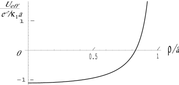
Figure 7: Effective potential in units of $e^{2}/(\kappa_{1}a)$ as a function of the distance from the axis of the cylindrical channel.

Remarkably, the effective potential is negative in the middle of the channel: $U_{eff}(0)\simeq-1.1e^{2}/(\kappa_{1}a)$. This means that the ions have a preference to go inside the channel, provided that the long–range part of the self–energy, $\propto L$, is not included. As before, the long–range part of the interaction energy is described by the field $\theta_{0}$, which is uniform in the transversal direction. This long–range part of the ion’s self–energy is related to the uniform electric field $E_{0}$ at distance $|x|\gg a$ from the charge. At smaller distance, $|x|\lesssim a$ the field is almost spherically symmetric, the same as in the bulk. As a result, the near vicinity of the charge, $|x|\lesssim a$, does not contribute to the excess self–energy. This “saves” the energy $1.1e^{2}/(\kappa_{1}a)$ per ion.

Let us return to the collective saddle point with the half–integer boundary charges, discussed in section III.2. Such boundary charges produce the electric field $E_{0}$, creating the OFP state. When an additional ion from the bulk enters the OFP state of the channel, its long range part of the self–energy is cancelled (by the field $E_{0}$ of the boundary charges), but the energy gain $1.1e^{2}/(\kappa_{1}a)$ remains. One may say that each charge reduces the length of the string of the field $E_{0}$ approximately by $a$, “saving” the energy $1.1e^{2}/(\kappa_{1}a)$. This energy gain comes on top of the entropy gain, discussed in section III.2. It leads to the increase of the effective concentration $\alpha_{eff}$, Eq. (78), in comparison with the naive geometrical one, $\alpha=cx_{T}\pi a^{\,2}$.

The ratio $\alpha_{eff}/\alpha$ for three choices of the hydrated ion radius $b$ is plotted versus $l_{B}/a$ in Fig. 8. One notices that for a reasonable for NaCl and KCl value Robinson $b=0.28l_{B}=0.2$ nm (used in section VIII for numerical estimates) the effective concentration may be up to $1.6$ times larger than the geometric one (the latter does not take into account the finite core radius). The results of the previous sections, summarized in section II, may be straightforwardly applied now with the $\alpha_{eff}$ substituted for $\alpha$.

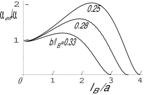
Figure 8: $\alpha_{eff}/\alpha$ as a function of $l_{B}/a$ for the three values of $b/l_{B}$.

VII Dynamics

Having discussed at length the activation barrier and its concentration and geometry dependence, we turn now to the pre-exponential factor in the expression for the channel resistance, Eq. (3). To this end we need a dynamical model for the ion’s motion inside the channel. It will also allow us to derive non–linear voltage–current relations, discussed in section III.5. We shall assume that the ions undergo dissipative brownian motion due to viscous friction with the water. The latter eventually transfers an excess momentum, the ions acquire in the external electric field, to the walls of the channel. Under these assumptions one may write the Langevin equation for the time–dependent coordinate of the $i$-th ion, $x_{i}(t)$:

$$\gamma\dot{x}_{i}=\sigma_{i}{V\over L}-{\partial U\over\partial x_{i}}+\eta_{i}(t)\,,$$ (81)

where $V$ is an externally applied voltage, $\gamma$ is the viscous friction coefficient and $\eta_{i}(t)$ is the Gaussian noise with the amplitude given by the fluctuation–dissipation theorem:

$$\langle\eta_{i}(t)\eta_{j}(t^{\prime})\rangle=2\gamma k_{B}T\delta_{ij}\delta(t-t^{\prime})\,.$$ (82)

In the absence of the activation barrier and the interparticle interactions these assumptions lead to the channel resistance given by the Drude formula: $R_{0}\equiv\gamma L/(2n)$. For a very small concentration $\alpha\to 0$, the ions cross the channel one by one overcoming the activation barrier given by Eq. (19) (but not interacting with other ions). The resistance associated with such a process is:

$$R=R_{0}\sqrt{\pi x_{T}\over L}\,\,e^{U_{L}(0)/(k_{B}T)}\,.$$ (83)

We shall assume furthermore that the resistance of the bulk reservoirs is negligible in comparison with that of the channel. This means that the boundary charges adjust to an instantaneous configuration of ions inside the channel. The boundary charge $q(t)$ is thus found from the minimum of the interaction energy: $\partial U(q,1-q)/\partial q=0$. We have assumed here that there is a single negative excess charge, travelling across the channel, and thus $q+q^{\prime}=1$. From Eq. (35) one then obtains:

$$q(t)={1\over 2}+{1\over L}\sum\limits_{i}\sigma_{i}x_{i}(t)\,.$$ (84)

This relation imposes the constraint on possible configurations of ions, $x_{i}$. Such a constraint was not included in the thermodynamic calculations. To discuss the dynamics one needs to define the equilibrium constrained free energy as:

$$e^{-\frac{F^{*}_{L}(q)}{k_{B}T}}\equiv\left\langle\delta\left({1\over L}\sum\limits_{i}\sigma_{i}x_{i}(t)+{1\over 2}-q\right)\right\rangle_{x_{i}},$$ (85)

where the angular brackets denote summation over number of ions and integrations over their coordinates with the weight given by Eq. (37). Introducing the Lagrange multiplier, one obtains the relation between the constrained and the unconstrained free energies:

$$e^{-\frac{F^{*}_{L}(q)}{k_{B}T}}={iL\over\pi x_{T}}\!\!\!\int\limits_{1/2-i\infty}^{1/2+i\infty}\!\!\!\!\!dQ\,\,e^{\,-\frac{F(Q)}{k_{B}T}+(Q-q)^{2}L/x_{T}}.$$ (86)

This integral may be evaluated in the saddle point approximation. From the saddle point equation one observes that the extensive parts of the constrained and the unconstrained free energies coincide at the two extrema, $q=0$ and $q=1/2$. This is the reason why one can discuss the activation barrier using the unconstrained free energy. The two free energies have distinct non-extensive parts, however, which must be kept to determine the pre-exponential factor.

We multiply now the constraint, Eq. (84), by the Drude resistance, $R_{0}=\gamma L/(2n)$, differentiate it over time and employ the Langevin equations (81). As a result:

$$R_{0}\dot{q}(t)=V-{1\over 2n}\sum\limits_{i}\sigma_{i}{\partial U\over\partial x_{i}}+\eta(t)\,,$$ (87)

where $\eta(t)\equiv(2n)^{-1}\sum_{i}\sigma_{i}\eta_{i}(t)$. This is the Gaussian noise with the correlator:

$$\langle\eta(t)\eta(t^{\prime})\rangle=\sum\limits_{i,j}{\sigma_{i}\sigma_{j}\over(2n)^{2}}\langle\eta_{i}(t)\eta_{j}(t^{\prime})\rangle=2k_{B}TR_{0}\,\delta(t-t^{\prime})\,.$$ (88)

It is thus the equilibrium Nyquist noise of the Drude resistor $R_{0}$.

Since the boundary charge, $q(t)$, is a weighted average of many uncorrelated fast functions, $x_{i}(t)$, one may assume that it possesses a slow dynamics. Thus, one may average out the fast motion of individual ions, $x_{i}(t)$, over the equilibrium distribution obtained for an instantaneous adiabatic value of $q(t)$. Averaging this way the second term on the r.h.s. of Eq. (87), one obtains footnote

$$R_{0}\dot{q}=V-{\partial F^{*}_{L}(q)\over\partial q}+\eta(t)\,.$$ (89)

The corresponding Fokker–Planck equation for the probability distribution function $P(q,t)$ is:

$$\partial_{t}P=-\partial_{q}I\,;\hskip 14.22636ptI\equiv{1\over R_{0}}\left[P\left(V-\partial_{q}F_{L}^{*}\right)-k_{B}T\partial_{q}P\right]\,.$$ (90)

Following the standard route Ambegaokar69 , one obtains for the linear resistance, $R=V/I$, in the stationary case, when the current $I$ is a constant:

$$R=R_{0}\int\limits_{0}^{1}\!\!dq\,e^{F_{L}^{*}(q)/(k_{B}T)}\int\limits_{0}^{1}\!\!dq\,e^{-F_{L}^{*}(q)/(k_{B}T)}\,.$$ (91)

The first integral here is dominated by the vicinity of the barrier top, $q=1/2$, while the second one – by the equilibrium state $q=0,1$. As a result, the resistance is given by:

$$R=R_{0}\,{\cal A}_{L}(\alpha)\,e^{\,U_{L}(\alpha)/(k_{B}T)}\,,$$ (92)

where $U_{L}(\alpha)=F_{L}(1/2)-F_{L}(0)$ is the activation barrier and factor ${\cal A}_{L}(\alpha)$ originates from the fluctuations around the extremal values of the integrals in Eqs. (86) and (91). Calculating the Gaussian integrals, one obtains for the pre-exponential factor:

$$\!\!{\cal A}_{L}(\alpha)={\pi x_{T}\over L}\,\frac{1+\omega_{b}^{2}}{\omega_{0}\omega_{b}}\,.$$ (93)

where $\omega_{0}^{2}\equiv\partial^{2}_{q}\epsilon^{(0)}_{q}|_{q=0}$ and $\omega_{b}^{2}\equiv-\partial^{2}_{q}\epsilon^{(0)}_{q}|_{q=1/2}$.

In the dilute limit, $\alpha\ll 1$, from Eqs. (50) and (52) one obtains: $\omega_{0}\approx 1-4\alpha^{2}$ and $\omega_{b}\approx(2\alpha)^{-1/2}$ and thus ${\cal A}_{L}(\alpha)\approx\pi x_{T}/(L\sqrt{2\alpha})$. The divergence at small $\alpha$ is terminated at $\alpha\sim x_{T}/L\ll 1$ (that is $nL\sim 1$, so there is less than one particle in the channel in average). At such a small concentration one can not assume that the $q(t)$ is a collective slow degree of freedom. Formally, the integrals in Eq. (91) can not be considered as Gaussian and the pre-factor saturates at ${\cal A}_{L}(0)=\sqrt{\pi x_{T}/L}$ as required by Eq. (83).

In the dense limit, $\alpha>1$, one finds that $F^{*}(q)\approx F(q)$ and thus $\omega_{0}=\omega_{b}=\pi\sqrt{f_{0}(\alpha)}/2\ll 1$. As a result, ${\cal A}_{L}(\alpha)=4x_{T}/(\pi Lf_{0}(\alpha))=\pi^{-1}k_{B}T/U_{L}(\alpha)$. The pre–factor grows with the concentration. This growth may be associated with the slow motion of the collective variable $q(t)$ near the top of the activation barrier. This result is applicable as long as $U_{L}(\alpha)/(k_{B}T)>1$.

To conclude, we found that the pre–exponential factor ${\cal A}(\alpha)$, cf. Eq. (92), exhibits the non–monotonous dependence on the salt concentration. It reaches a flat minimum at $\alpha\approx 0.2$, where ${\cal A}_{L}(.2)\approx 8x_{T}/L$ and increases both for smaller and larger concentrations. Employing Eq. (90), one may go beyond the linear response theory and discuss non–linear voltage–current relation. Since such a derivation is relatively standard Ambegaokar69 we do not provide it here. The corresponding results are listed in sections I and III.5.

VIII Conclusions

In this paper we suggested a theory of the salt–induced reduction of the transport activation barrier in the water–filled channels in a media with much smaller dielectric constant, than that of the water. Our theory is based on one–dimensional nature of the electric field in the channel. We have derived a universal dependencies of the barrier height $U_{L}(\alpha)$ as a function of the dimensionless parameter $\alpha$, given by Eq. (11). They are presented in section II. Remarkably, when the channel radius $a$ grows, the one–dimensional character of the problem remains valid until at some $\alpha$ the barrier $U_{L}(\alpha)$ becomes smaller than $k_{B}T$. In this sense one may say that transition from one-dimensional channel to the bulk is governed solely by $\alpha$ (and not any other parameter, e.g. $\xi/a$, or $x_{D}/a$, etc.)

Now we would like to consider a few examples of application of our theory to water–filled pores. The first one is $\alpha$-hemolysin, a passive protein channel in lipid membranes. As we mentioned above, for the water–filled channels in lipid membranes $\xi\simeq 6.8\,a$. For the $\alpha$-hemolysin $L=5$ nm, $a=0.75$ nm and thus $L/\xi\approx 1$. For this case, according to Eq. (8) we obtain $U_{\infty}(0)=6.8k_{B}T_{r}$ and according to Eq. (9) $U_{L}(0)=0.46U_{\infty}(0)=3.1k_{B}T_{r}$, where $T_{r}$ is the room temperature. To describe the effect of salt one can use the curve for $L/\xi=1$ in Fig. 4 with $\alpha_{eff}$ substituted for $\alpha$. The point where $U_{L}(\alpha)/U_{L}(0)=0.5$, corresponds to $\alpha_{eff}=0.2$. For $a=0.75$ nm, $l_{B}/a=0.93$ Fig. 8 gives $\alpha=0.8\alpha_{eff}=0.16$, corresponding to $c=0.37$ M and the bulk concentration of salt $c_{0}=0.46$ M. Thus, it is enough to have $0.5$ M of salt to reduce the activation exponent by the factor of two.

The second example is a water–filled nanopore made in a silicon film  Li ; Storm . Such nanopores are considered in nanoscience for the transport of DNA, in salty water Timp . We are concerned only with the transport of small ions in a e.g. KCl solution. Let us assume that $a=1$ nm and the length $L=20$ nm. Silicon oxidizes around the channel, giving $\kappa_{2}\simeq 4$ and $\kappa_{1}/\kappa_{2}=20\gg 1$. Using Eq. (7), we find $\xi=4.75\,a$. This gives $L/\xi\simeq 4$. For this case, according to Eq. (8) we obtain $U_{\infty}(0)=3.6k_{B}T_{r}$ and Eq. (9) results in $U_{L}(0)=0.96U_{\infty}(0)=3.4k_{B}T_{r}$. Effect of salt is given by the top full curve in Fig. 4, corresponding to $L/\xi=4$. In this case, $U_{L}(\alpha)/U_{L}(0)=0.5$ at $\alpha_{eff}=0.4$ or at $\alpha=0.36$ (as we see in Fig. 8 for $l_{B}/a=0.7$ the ratio $\alpha_{eff}/\alpha=1.12$). This requires $c=0.26$ M and $c_{0}=0.31$ M.

The third example is a water–filled nanopore with $L=40$ nm and $a=1.5$ nm in cellulose acetate film used for inverse osmosis desalination. Let us take $\kappa_{2}\simeq 2$ so that $\xi\simeq 6.8\,a\simeq 10$ nm , $L/\xi\simeq 4$, $U_{L}(0)=0.96U_{\infty}(0)\approx 3k_{B}T_{r}$. Effect of salt is again given by the top full curve in Fig. 4 and $U_{L}(\alpha)/U_{L}(0)=0.5$ at $\alpha_{eff}=0.4$ which in this case corresponds to $\alpha=0.38$. This happens at $c=0.69$ M and $c_{0}=0.73$ M.

The last example, we want to consider, is the gramicidin-A-like channel in a lipid membrane. In this case we use $L=2.5$ nm, $a=0.3$ nm and obtain $L/\xi=1.2$. According to Eq. (8) the barrier $U_{\infty}(0)=17k_{B}T_{r}$ and according to Eq. (9): $U_{L}(0)=0.55\,U_{\infty}(0)=9.4k_{B}T_{r}$. We see that, because of the very small width, we deal with much higher barriers. On the other hand, at such a small $a$ even the concentration of salt $c_{0}$ close to the saturation limit of $6$ M and corresponding $c=5.2$ M we can reach only $\alpha=0.06$ or $\alpha_{eff}=0.084$ (for this case $l_{B}/a=2.3$ and according to Fig. 8 $\alpha_{eff}/\alpha=1.4$). At this $\alpha_{eff}$ interpolating between curves for $L/\xi=1$ and $L/\xi=1.5$ we arrive at $U_{L}(\alpha)=0.83U_{L}(0)=7.8k_{B}T_{r}$. Thus, the effect of salt on a narrow channel is weak. This could be anticipated from Eq. (11), if we rewrite it as $\alpha=\pi(cl_{B})^{3}(a/l_{B})^{4}$ and take into account that $cl_{B}^{3}\leq 1$, even at the saturation limit $c_{0}=6$ M. Contrary to the case where $a/l_{B}\geq 1$ and the range $\alpha>1$ is accessible, in the opposite limit $a/l_{B}\lesssim 1$ the parameter $\alpha$ is bound to be small footnote2 .

In this paper we considered only channels without charges fixed on their walls. Methods used here can be easily applied for channels with fixed charges of one or both signs. We will address such channels in the next publication.

IX Acknowlegments

We are grateful to A. L. Efros, M. M. Fogler, L. I. Glazman, A. Yu. Grosberg, A. Meller, S. Teber, Ch. Tian and M. Voloshin for numerous useful discussions. A. K. is supported by the A.P. Sloan foundation and the NSF grant DMR–0405212. A. I. L. is supported by NSF Grants No. DMR-0120702 and DMR-0439026. B. I. S is supported by NSG grant DMI-0210844.

References

- (1) L. Stryer, Biochemistry, 4-th edition (chapter 12), Freeman Co., NY (1995).
- (2) B. Hille, Ion Channels of Excitable Membranes, Sinauer Associates, Sunderland, MA (2001).
- (3) L. Dresner, Desalination 15, 39 (1974); A. E. Yaroshchuk, Adv. Colloid and Interface Science 85, 193 (2000).
- (4) J. Li, D. Stein, C. McMullan, D. Branton, M. J. Aziz, and J. A. Golovchenko, Nature 412, 166 (2001).
- (5) A. J. Storm, J. H. Chen, X. S. Ling, H. W. Zandergen, and C. Dekker, Nat. Mater. 2, 537 (2003).
- (6) A. Aksimentiev, J. B. Heng, G. Timp, and K. Shulten, Biophys. J. 87, 2086 (2004).
- (7) Y. Cui, L.J. Lauhon, M.S. Gudiksen, J. Wang, and C.M. Lieber, Appl. Phys. Lett. 78, 2214-2216 (2001).
- (8) We are grateful to F. M. Peeters for attracting our attention to this application.
- (9) A. Parsegian, Nature 221, 844-846 (1969).
- (10) D. G. Levitt, Biophys J. 22, 209 (1978).
- (11) P. C. Jordan, Biophys J. 39, 157 (1982).
- (12) B. Nadler, U. Hollerbach, and R. S. Eisenberg, Phys. Rev. E. 68, 021905 (2003).
- (13) A. V. Finkelstein and O. B. Ptitsyn, Protein Physics (chapter 12). Academic Press, An Imprint of Elsevier Science; Amsterdam (2002).
- (14) A. V. Finkelstein, D. N. Ivankov, and A. M. Dykhne, in preparation.
- (15) S. Teber, cond-mat/0501662.
- (16) A. Lenard, J. Math. Phys. 2, 682 (1961).
- (17) S. F. Edwards and A. Lenard, J. Math. Phys. 3, 778 (1962).
- (18) W. Apel, H. U. Everts, and H. Schultz, Z. Phys. B 34, 183 (1979).
- (19) R. A. Robinson, R. H. Stokes Electrolyte solutions, Chapter 9, Butterworths, London (1959).
- (20) J. Frenkel, Phys. Rev. 54, 647 (1938).
- (21) M. Abramovitz, A. Stegun (Eds.), Handbook of Mathematical Functions, (chapter 20). Dover, NY 1965.
- (22) I. Affleck, Phys. Rev. Lett. 46, 388-391 (1981).
- (23) W. R. Smythe, Static and Dynamic Electricity, 3-rd edition (chapter V), McGraw-Hill Book Company (1968). A. A. Kornyshev and M. A. Vorotyntsev, J. Phys. C: Solid State Phys. 12, 4939 (1979).
- (24) V. Ambegaokar and B. I. Halperin Phys. Rev. Lett. 22, 1364-1366 (1969).
-
(25)
To carry out this averaging one parameterizes the ions
coordinates as , where the constraint (84) is reduced
to . The second term on the
r.h.s. of Eq. (87) may be written now as:
where we employed that . Averaging over the equilibrium distribution function , one finds: . - (26) Another possible application of our theory is the transport in single-crystal silicon nanowires Lieber suspended in air between two conductors. They have nm and lengths up to several microns. In this case, and so that the ratio is relatively large. We will address this application in a future publication.