Generating Function for Particle-Number Probability Distribution in Directed Percolation

Abstract

We derive a generic expression for the generating function (GF) of the particle-number probability distribution (PNPD) for a simple reaction diffusion model that belongs to the directed percolation universality class. Starting with a single particle on a lattice, we show that the GF of the PNPD can be written as an infinite series of cumulants taken at zero momentum. This series can be summed up into a complete form at the level of a mean-field approximation. Using the renormalization group techniques, we determine logarithmic corrections for the GF at the upper critical dimension. We also find the critical scaling form for the PNPD and check its universality numerically in one dimension. The critical scaling function is found to be universal up to two non-universal metric factors.

I Introduction

In the last decades, the statistical mechanics of non-equilibrium models characterized by large scale space-time fluctuations and absorbing phase transition has been studied extensively with numerical and analytical tools Hinrichsen (2000). The directed percolation (DP) universality class covers a large variety of models of this type, which have short range interactions, a single absorbing state, and a scalar order parameter J81 ; G82 . The DP conjecture has been extended to models with multiple components and even multiple absorbing states, unless there is an additional symmetry and a conservation law. Nevertheless we should mention that there is at least one exception in the case of more elaborated interactions HH ; Janssen et al. ; Park04 .

Besides various numerical techniques, the response functional formalism combined with the renormalization group (RG) techniques is one of the powerful analytical tool to explore the asymptotic properties near criticality for these models Cardy and Täuber (1998); Cardy (1999); Tauber05 ; Janssen (2000); Janssen05 . The DP universality is described by the Reggeon field theory which has been investigated in details by many researchers Hinrichsen (2000). Its upper critical dimension is known to be 4 and the values of the critical exponents were obtained up to ${\cal O}({\epsilon}^{2})$ with space dimension $d=4-\epsilon$ J81 ; JKO99 . The leading logarithmic corrections at the upper critical dimension are also available in the literature Wil98 ; Janssen and Stenull (2004) and tested numerically Lübeck (2004). Recently the same field-theoretical formalism was successfully applied to identify and calculate the survival probability and the mean number of particles, which are the central quantities of interest in the damage-spreading (DS) type dynamics Janssen (2003); Janssen and Stenull (2004).

The aim of this paper is to explore in the same framework a more general and useful quantity in the DS type dynamics; the generating function (GF) of the particle-number probability distribution (PNPD). In principle, all moments of the number of particles including the survival probability can be derived from the GF. We start from a lattice description of a reaction diffusion model that belongs to the DP universality class. Then, we use the bosonic operator formalism Cardy (1999) to represent the master equation and the associated field theory to define the generating function (GF) of the PNPD. With a single particle initially, we derive the GF of the PNPD as an infinite series of multi-point Green functions. This series can be summed up explicitly under the tree (mean-field) approximations into a complete form.

Assuming the generic critical scaling property of the Green functions, we obtain the critical scaling form of the PNPD. Using the RG techniques, we calculate the leading logarithmic corrections for the critical GF at the upper critical dimension. Our results are consistent with recent reports for the survival probability and the average number of particles by Janssen and Stenull Janssen and Stenull (2004); Janssen (2003).

The conventional RG analysis suggests that the critical scaling function for the PNPD should be universal up to two non-universal metric factors which microscopic details of the models are integrated into. We check this universality numerically in one dimension for two variants of bosonic DP models and also for the hard core DP models where the site occupancy of particles is restricted to one. Numerical simulations show that all the models form a universality very nicely at criticality with only two adjusting parameters.

The paper is organized as follows: Section  II introduces the model and defines the GF for the PNPD. Secion  III is devoted to the derivation of the series expansion of the GF in terms of connected Green functions. In Sec. IV, we derive the mean field solution and present the logarithmic corrections to the scaling in the critical state at the upper critical dimension for the first three moments of the PNPD. In Sec. V, we analyze the scaling form of the critical PNPD, using the RG equations and test it numerically in one dimension for both bosonic models and hard core models. We present the conclusion in Sec. VI and the technical details for the calculation of the logarithmic corrections in the Appendix.

II General formalism

We consider a reaction diffusion model (the Gribov process) J81 ; G82 that belongs to the DP universality. It is defined on a $d$-dimensional lattice with $N^{d}$ sites which may be either vacant or occupied by particles. The evolution rule is summarized in the stoichiometric notation as

$$A\varnothing \stackrel{{\scriptstyle D_{l}}}{{\longleftrightarrow}}\varnothing A\ ,$$

$$A \stackrel{{\scriptstyle\lambda_{a}}}{{\longrightarrow}}\varnothing\ ,$$

$$2A \stackrel{{\scriptstyle\lambda_{c}}}{{\longrightarrow}}A\ ,$$ (1)

$$A \stackrel{{\scriptstyle\lambda_{b}}}{{\longrightarrow}}2A\ ,$$

where $D_{l}$ is the nearest neighbor hopping (diffusion) rate, $\lambda_{a}$ is the annihilation rate for a particle, $\lambda_{c}$ is the coagulation rate for two particles at a site, and $\lambda_{b}$ is the branching rate.

A microscopic state of the system is defined by the set of particle numbers at each lattice site: ${\bf n}=\{n_{i}\}$. The time evolution of the probability distribution $P({\bf n},t)$ can be described by the master equation for the state vector $|\Psi(t)\rangle=\sum_{\bf n}P({\bf n},t)|{\bf n}\rangle$ at time $t$:

$$\frac{d|\Psi\rangle}{dt}=-H|\Psi\rangle\ .$$ (2)

The evolution operator $H$ can be written in terms of bosonic operators as

$$H = D_{l}\sum_{\langle ij\rangle}(a^{\dagger}_{i}-a^{\dagger}_{j})(a_{i}-a_{j})-\lambda_{a}\sum_{i}(a_{i}-a^{\dagger}_{i}a_{i})$$ (3)

$$-\lambda_{c}\sum_{i}(a^{\dagger}_{i}a^{2}_{i}-{a^{\dagger}}^{2}_{i}a^{2}_{i})-\lambda_{b}\sum_{i}({a^{\dagger}}^{2}_{i}a_{i}-{a^{\dagger}}_{i}a_{i})\ ,$$

where $a_{i}(a^{\dagger}_{i})$ is the annihilation (creation) operator of bosonic particles, satisfying the commutation relation $[a_{i},a^{\dagger}_{j}]=\delta_{ij}$.

The average of a quantity $O$ at time $t$ is computed by the formula

$$\langle O\rangle_{t}=\langle 0|e^{\sum_{i}a_{i}}{\hat{O}}e^{-tH}|\Psi(0)\rangle$$ (4)

for a given initial state $|\Psi(0)\rangle$ Cardy and Täuber (1998); Cardy (1999); Tauber05 , where $|0\rangle$ represents the vacuum state and ${\hat{O}}$ is the operator representation of the quantity $O$. Similarly, one can easily derive the probability that the system has $n$ particles on the lattice at time $t$ Howard98 as

$$p(n,t)=\frac{1}{n!}\langle 0|\Bigl{(}\sum_{i}a_{i}\Bigr{)}^{n}e^{-tH}|\Psi(0)\rangle\ ,$$ (5)

and its generating function (GF) is defined as

$$F(s,t)=\sum_{n=0}s^{n}p(n,t)=\langle 0|e^{\sum_{i}sa_{i}}e^{-tH}|\Psi(0)\rangle\ .$$ (6)

III The expansion of the generating function

It is well known that the calculation of the average becomes simpler by moving the factor $e^{\sum_{i}a_{i}}$ in Eq. (4) to the rightmost position. Since $e^{a}a^{\dagger}=(a^{\dagger}+1)e^{a}$, this move results in shifting $a^{\dagger}\rightarrow a^{\dagger}+1$ in the operators ${\hat{O}}$ and $H$. We use the same trick to calculate the GF in Eq. (6), and then

$$F(s,t)=\langle 0|e^{\sum_{i}(s-1)a_{i}}e^{-tH_{s}}e^{\sum_{i}a_{i}}|\Psi(0)\rangle\ ,$$ (7)

where the shifted Hamiltonian $H_{s}(a^{\dagger},a)=H(a^{\dagger}+1,a)$.

Through the standard coherent-state path integral formulation Cardy (1999); Tauber05 , one can find the shifted action $S(\bar{\phi},\phi)$ such that the path integral is weighed by $e^{-S}$ as

$$S(\bar{\phi},\phi)=\int dt\left[\sum_{i}\bar{\phi}_{i}\partial_{t}\phi_{i}+H_{s}(\bar{\phi},\phi)\right]$$

$$=\int dt\left[\sum_{i}\bar{\phi}_{i}\partial_{t}\phi_{i}+D_{l}\sum_{\langle ij\rangle}(\bar{\phi}_{i}-\bar{\phi}_{j})(\phi_{i}-\phi_{j})\right.$$

$$\left.+\!\sum_{i}\left\{(\lambda_{a}-\lambda_{b})\bar{\phi}_{i}\phi_{i}\!+\!\lambda_{c}\bar{\phi}_{i}\phi_{i}^{2}\!-\!\lambda_{b}{\bar{\phi}_{i}}^{2}\phi_{i}\!+\!\lambda_{c}{\bar{\phi}_{i}}^{2}\phi_{i}^{2}\right\}\right].$$ (8)

For the calculation of the asymptotic properties, the action is taken formally in the continuum limit with the transformations

$$\sum_{i}\rightarrow b^{-d}\!\int dx^{d},\ \ f_{x_{i}+be_{j}}-f_{x_{i}}\rightarrow b\nabla_{x_{j}}f(x),$$

$$\phi_{i}(t)\rightarrow b^{d}\phi(x,t),\quad\bar{\phi}_{i}(t)\rightarrow\bar{\phi}(x,t)\ ,$$ (9)

$$D=b^{2}D_{l},\ \ \mu=\lambda_{a}-\lambda_{b},\ \ g^{\prime}=b^{d}\lambda_{c},\ \ g^{\prime\prime}=\lambda_{b},$$

where $b$ is the lattice constant and $e_{j}$ is the unit vector along the $j$ axis. In the continuum limit, the action reads

$$S= \int dxdt\left[\bar{\phi}(x,t)\partial_{t}\phi(x,t)+D(\nabla\bar{\phi}(x,t))(\nabla\phi(x,t))\right.$$

$$\left.+\mu\bar{\phi}(x,t)\phi(x,t)+\frac{1}{2}g^{\prime}\bar{\phi}(x,t)\phi^{2}(x,t)\right.$$

$$\left.-\frac{1}{2}g^{\prime\prime}{\bar{\phi}}^{2}(x,t)\phi(x,t)\right],\$$ (10)

where the term $g^{\prime}{\bar{\phi}}^{2}\phi^{2}$ is dropped as being irrelevant. The coupling constants $g^{\prime}$ and $g^{\prime\prime}$ can be reduced to one coupling constant $g=\sqrt{g^{\prime}g^{\prime\prime}}$ by rescaling the fields as follows: $\phi\to\alpha\phi$, $\bar{\phi}\to\alpha^{-1}\bar{\phi}$, with $\alpha=\sqrt{g^{\prime\prime}/g^{\prime}}$. The rescaled “symmetric” action is then invariant under the time reversal transformation: $t\to-t$, $\phi\to-\bar{\phi}$, $\bar{\phi}\to-\phi$.

Consider the GF with one particle initially: $|\Psi(0)\rangle=a_{0}^{\dagger}|0\rangle$. Then, we have

$$F(s,t)=\langle 0|e^{\sum_{i}(s-1)a_{i}}e^{-tH_{s}}(a^{{\dagger}}_{0}+1)|0\rangle$$

$$=1+\langle 0|e^{\sum_{i}(s-1)a_{i}}e^{-tH_{s}}a^{{\dagger}}_{0}|0\rangle$$

$$=1+\sum_{p=1}\frac{(s-1)^{p}}{p!}\sum_{i_{1},\dots,i_{p}}\langle 0|a_{i_{1}}(t)\dots a_{i_{p}}(t)e^{-tH_{s}}a^{\dagger}_{0}(0)|0\rangle\ ,$$ (11)

where we used the relations $H_{s}|0\rangle=0$ and $\langle 0|H_{s}$=0 because each term in $H_{s}$ has $a^{\dagger}$ to the left and $a$ to the right. In the path-integral formulation, the above correlation functions are simply connected Green functions (cumulants) with the shifted action in Eq. (8). In the continuum limit with the symmetric action, the GF is written as

$$F(s,t)=1+\sum_{p=1}\frac{(s-1)^{p}}{p!}\alpha^{p-1}$$

$$\times\int dx_{1},\dots dx_{p}G^{(p,1)}(x_{1},t,\dots x_{p},t;0,0)\ ,$$ (12)

where

$$G^{(p,1)}(x_{1},t,\dots x_{p},t;0,0)=\langle\phi(x_{1},t)\dots\phi(x_{p},t)\bar{\phi}(0,0)\rangle$$ (13)

are the connected Green functions for the symmetric action and the factor $\alpha=\sqrt{g^{\prime\prime}/g^{\prime}}$ stems from the rescaling of the fields.

Close to the critical point, we can use the renormalized Green functions of which the scaling behavior is known. Then, we have

$$G^{(p,1)}(x_{1},t,\dots x_{p},t;0,0)$$

$$=Z^{p/2}_{\phi}Z^{1/2}_{\bar{\phi}}G^{(p,1)}_{R}(x_{1},t,\dots x_{p},t;0,0)$$

$$=Z^{p/2}_{\phi}Z^{1/2}_{\bar{\phi}}t^{-p\frac{\beta}{\nu_{\parallel}}-\frac{\beta^{\prime}}{\nu_{\parallel}}}\mathcal{G}^{(p,1)}(x_{1}/t^{1/z},\dots x_{p}/t^{1/z})\ ,$$ (14)

where $Z_{\phi}$, $Z_{\bar{\phi}}$ are the fields renormalization factors that are equal for the time reversal symmetric theory and we have used the scaling property of the renormalized Green functions close to the critical point as

$$G^{(p,1)}_{R}(x_{1},t_{1},\dots x_{p},t_{p};x_{0},t_{0})=|\mu|^{p\beta+\beta^{\prime}}$$

$$\times H(|\mu|^{\nu_{\perp}}x_{1},|\mu|^{\nu_{\parallel}}t_{1},\dots)\ ,$$ (15)

where $\mu$ is the deviation from the critical point, and $\beta$, $\beta^{\prime}$, $\nu_{\parallel}$, $\nu_{\perp}$ and $z$ are the standard critical exponents defined in Ref. Hinrichsen (2000).

The generating function can be written now as

$$\bar{F}(s,t)\equiv F(s,t)-1$$

$$=\sum_{p=1}\frac{(s-1)^{p}}{p!}\alpha^{p-1}Z^{p/2}_{\phi}Z^{1/2}_{\bar{\phi}}t^{-p(\frac{\beta}{\nu_{\parallel}}-\frac{d}{z})-\frac{\beta^{\prime}}{\nu_{\parallel}}}A^{(p,1)}$$

$$=t^{-\frac{\beta^{\prime}}{\nu_{\parallel}}}Z^{1/2}_{\phi}Z^{1/2}_{\bar{\phi}}\left[\sum_{p=1}\frac{(s-1)^{p}}{p!}(\alpha Z_{\phi}^{1/2})^{p-1}t^{p(\frac{d}{z}-\frac{\beta}{\nu_{\parallel}})}A^{(p,1)}\right]\ ,$$ (16)

where

$$A^{(p,1)}=\int dx_{1}\dots,dx_{p}\mathcal{G}^{(p,1)}(x_{1},\dots,x_{p})\ .$$ (17)

This expression shows that $\bar{F}(s,t)$ can be renormalized by multiplication with $Z^{-1/2}_{\phi}Z^{-1/2}_{\bar{\phi}}$ after the parameter $\alpha$ is renormalized as $\alpha_{R}=Z^{1/2}_{\phi}\alpha$ .

IV Mean field approximation and logarithmic corrections

IV.1 Mean-field solution

In Eq. (16), the GF is expressed as a formal series whose convergence property depends on the coefficients $A^{(p,1)}$. As a first step to study this series, we calculate the mean field (MF) solution for the GF. In this approximation, we consider only the tree diagrams for the multi-point correlation function $G^{(p,1)}$ in Eq. (12).

Figure 1: The first three tree diagrams used in the mean-field approximation.

The lowest order approximation of the $(p,1)$ Green function can be obtained by connecting $p-1$ vertices of type $\bar{\phi}^{2}\phi$ with free two point Green functions, as shown in Fig. 1 where each line is associated with the free two-point $(1,1)$ Green function in the momentum space as

$$G(k,t)=\theta(t)e^{-t(Dk^{2}+\mu)}.$$ (18)

For the sum of tree diagrams we can easily obtain an integral recurrence equation for the GF by resuming the diagrams after the first vertex from the right in the tree, which is

$$\bar{F}(s,t)=\bar{F}(s,0)e^{-\mu t}+\frac{1}{2}g^{\prime\prime}\int_{0}^{t}dt^{\prime}{\bar{F}(s,t-t^{\prime})}^{2}G(k=0,t^{\prime}),$$ (19)

that is equivalent with the differential equation

$$\frac{d}{dt}\bar{F}(s,t)=-\mu\bar{F}(s,t)+\frac{1}{2}g^{\prime\prime}{\bar{F}(s,t)}^{2}.$$ (20)

With the single particle initial condition $F(s,0)=s$ $(\bar{F}(s,0)=s-1)$, one can find the exact solution for the GF as

$$F(s,t)=1+\frac{(s-1)e^{-\mu t}}{1-(s-1)\frac{g^{\prime\prime}}{2\mu}(1-e^{-\mu t})}\ .$$ (21)

By inverting the GF in Eq. (6), we find the PNPD as

$$p(n,t)=\frac{e^{-\mu t}}{(1+\frac{g^{\prime\prime}}{2\mu}(1-e^{-\mu t}))^{2}}\left(\frac{\frac{g^{\prime\prime}}{2\mu}(1-e^{-\mu t})}{1+\frac{g^{\prime\prime}}{2\mu}(1-e^{-\mu t})}\right)^{n-1},$$ (22)

for $n\geq 1$. At criticality ($\mu=0$), the PNPD behaves in the asymptotic limit (large $t$) as

$$p(n,t)\approx\left(\frac{2}{g^{\prime\prime}t}\right)^{2}e^{-\frac{2(n-1)}{g^{\prime\prime}t}}.$$ (23)

The survival probability $p_{s}(t)$ that the system is active at time $t$ can be derived from the expression $p_{s}(t)=1-p(0,t)$$=1-F(0,t)$. From Eq. (21), we find

$$p_{s}(t)=\frac{e^{-\mu t}}{1+\frac{g^{\prime\prime}}{2\mu}(1-e^{-\mu t})}\ .$$ (24)

We also find the mean number of particles $N(t)=\langle n\rangle=\sum_{n}np(n,t)=\partial F/\partial s|_{s=1}$ as

$$N(t)=e^{-\mu t}.$$ (25)

Similarly, all higher moments $\langle n^{k}\rangle$ can be obtained by differentiating the GF with respect to $s$ and taking the $s\to 1$ limit.

At criticality, the survival probability decays algebraically as

$$p_{s}(t)=\frac{1}{1+g^{\prime\prime}t/2}\approx\frac{2}{g^{\prime\prime}}t^{-1}\ ,$$ (26)

while $N(t)$ remains a constant of unity. This is consistent with other MF predictions for the dynamic scaling exponents: $\delta_{MF}=1$ and $\eta_{MF}=0$ Hinrichsen (2000).

Near criticality, we find, for the large $t$ limit, that $p_{s}(t)\approx(2\mu/g^{\prime\prime})e^{-\mu t}$ in the absorbing side $(\mu\gtrsim 0)$ and $p_{s}(t)\approx(2|\mu|/g^{\prime\prime})(1+e^{-|\mu|t})$ in the active side $(\mu\lesssim 0)$. These results are fully consistent with the recent results by Janssen Janssen (2003).

IV.2 Logarithmic corrections to critical scaling

At the critical dimension, where the coupling constant is dimensionless, the MF solution (21) can be improved systematically at large time with the help of the renormalization group equations by adding the one-loop correction. A detailed account of this procedure has been presented recently in reference Janssen and Stenull (2004). In our case we use one-loop approximation for the GF, combined with the two-loop Wilson functions taken from literature. The details of the calculation for one-loop GF and its asymptotic scaling derived with the help of RG equations are presented in the Appendix. In this section we present, for the critical state, in a parametric form, the leading order expressions of the survival probability, $p_{s}(t)$, and of the first two moments of the particle number distribution, $N(t)$, $N_{2}(t)$, which might be of interest for numerical experiments.

From Eq. (A) we have at large $t$

$$p_{s}(t) =-\bar{F}(0,t)$$

$$=\frac{4N^{\prime}}{\bar{D}t}w^{-1}e^{c_{0}w^{2}+O(w^{4})}\left(1+(3\ln X_{0}-9/2)w^{2}\right)$$

$$+O(w^{-5/6}t^{-2})\ ,$$ (27)

$$N(t) =\frac{\partial\bar{F}(s,t)}{\partial s}\Big{|}_{s=1}$$

$$=N^{\prime}w^{-1/3}e^{c_{1}w^{2}+O(w^{4})}(1+(\ln X_{0}+1)w^{2})\ ,$$ (28)

$$N_{2}(t) =\frac{\partial^{2}\bar{F}(s,t)}{\partial s^{2}}\Big{|}_{s=1}+N(t)$$

$$=\frac{1}{2}N^{\prime}\bar{D}tw^{1/3}e^{c_{2}w^{2}+O(w^{4})}$$

$$\times(1-(\ln X_{0}-4)w^{2})+O(w^{-1/3})\ ,$$ (29)

where $w$ depends on time $t$ through Eqs. (64, 65). In the above expressions, the universal constants $c_{0}$, $c_{1}$, $c_{2}$ are defined in terms of the coefficients of the Wilson functions, Eqs (46- 48), and have the values

$$c_{0} =\frac{1}{48}\left(7-34\ln\frac{4}{3}\right)$$ (30)

$$c_{1} =-\frac{1}{144}\left(25+322\ln\frac{4}{3}\right)$$ (31)

$$c_{2} =-\frac{1}{144}\left(71+542\ln\frac{4}{3}\right)\ .$$ (32)

The remaining $N^{\prime}$, $\bar{D}$, $X_{0}$ and $t_{0}$ are non-universal constants whose detailed origins can be explored in the Appendix.

We make the observation that Eqs. (IV.2,28) are equivalent with the expressions of Ref. Janssen and Stenull (2004) after the change of variable $w\to(w/8)^{1/2}$.

V Critical scaling functions for the PNPD

Since the GF of the PNPD is renormalizable, see Eq. (16), we can use the RG equation to find its scaling properties in the critical state. At large $t$, we can extract the scaling property of the PNPD through the GF scaling behavior.

A dimensional analysis with Eq. (16) suggests the following form for the GF

$$\bar{F}(s,t)=yf(D\kappa^{2}t,y\alpha\kappa^{-d/2},u)\ ,$$ (33)

where $\kappa^{-1}$ is an arbitrary length, $u$ is the dimensionless coupling constant (see Appendix), and $y=s-1$.

The independence of the bare $\bar{F}$ on $\kappa$ yields the renormalization group equation

$$\kappa\frac{\partial}{\partial\kappa}\left(yZ_{\phi}f(D\kappa^{2}t,y\alpha\kappa^{-d/2},u)\right)=0$$ (34)

or, in more details, we have

$$\left(\gamma_{\phi}+\kappa\frac{\partial}{\partial\kappa}+\gamma_{D}D\frac{\partial}{\partial D}+\gamma_{\alpha}\alpha\frac{\partial}{\partial\alpha}+\beta(u)\frac{\partial}{\partial u}\right)$$

$$\times yf(D\kappa^{2}t,y\alpha\kappa^{-d/2},u)=0$$ (35)

where $\gamma_{\phi}=\kappa\partial_{\kappa}\ln Z_{\phi}$, $\gamma_{D}=\kappa\partial_{\kappa}\ln Z_{D}$, $\gamma_{\alpha}=\gamma_{\phi}/2$ and $\beta(u)=\kappa\partial_{\kappa}u$, with $Z_{\phi}$, $Z_{D}$ the standard renormalization factors Cardy (1999).

Equation (33) gives the following relations for the differential operators

$$\kappa\frac{\partial}{\partial\kappa} =2t\frac{\partial}{\partial t}-\frac{d}{2}\alpha\frac{\partial}{\partial\alpha}\ ,$$

$$D\frac{\partial}{\partial D} =t\frac{\partial}{\partial t}\ ,$$ (36)

$$\alpha\frac{\partial}{\partial\alpha} =y\frac{\partial}{\partial y}-1,$$

hence the generic solution at the fixed point is

$$\bar{F}(s,t)=t^{-\frac{\gamma^{*}_{\phi}}{2+\gamma^{*}_{D}}}y\bar{f}\left(yt^{\frac{d/2-\gamma^{*}_{\phi}/2}{2+\gamma^{*}_{D}}}\right),$$ (37)

where starred parameters are values of corresponding $\gamma$ functions at the fixed point.

Using the standard RG technique Amit84 , the function $\bar{f}$ up to $O(\epsilon)$ and a multiplicative non-universal amplitude can be obtained by replacing in Eq. (45) $u^{2}\to\epsilon/12$, $rt$ $\to$ $-C_{y}yt^{(d/2-\gamma^{*}_{\phi}/2)/(2+\gamma^{*}_{D})}$ and $t/\bar{t}\to 1$; where $C_{y}>0$ is a second non-universal amplitude, $\gamma^{*}_{\phi}=-\epsilon/6$ and $\gamma^{*}_{D}=-\epsilon/12$ up to $O(\epsilon)$ Janssen05 .

Since the difference between $p(n,t)$ and $p(n+1,t)$ for large $t$ is small, the generating function $\bar{F}$ can be approximated by a Laplace transform with the parameter $\omega=-\ln s$. Applying the inverse Laplace transform in which we approximate $y\approx-\omega$, we obtain

$$p(n,t)=t^{-d/z}\bar{g}\left(\frac{n}{t^{d/(2z)+\eta/2}}\,\right)$$ (38)

where we have introduced the exponents $z=2+\gamma^{*}_{D}$ and $\eta=-\gamma^{*}_{\phi}/(2+\gamma^{*}_{D})$ defined by scaling properties of the two point Green function Cardy (1999). Equation (38) along with the relation $p_{s}(t)=\int dnp(n,t)$ gives the survival exponent $\delta=(d/z-\eta)/2$, which is the well-known hyperscaling relation.

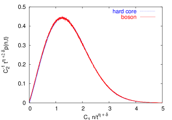
Figure 2: Critical scaling function for the PNPD in one dimension with full lines for boson models (pair annihilation and pair coagulation) and with dashed lines for hard-core particles models (the contact process and the bond directed percolation). The curve corresponding to the contact process is chosen for reference, and the other data sets are plotted for the best overlap with the reference curve by varying the constants $C_{1}$ and $C_{2}$.

The scaling analysis predicts that the critical PNPD at large $t$ has the form

$$p(n,t)=\frac{C_{2}}{t^{\eta+2\delta}}\;g\!\left(C_{1}\frac{n}{t^{\eta+\delta}}\right)\ ,$$ (39)

where $C_{1}$, $C_{2}$ are two non-universal metric factors which depend on the values of the microscopic parameters and $g$ is the universal scaling function. The two-scale factor universality is worth while to be mentioned at this point. Since we are interested in the dynamic behavior of the system, there are, in general, three independent metric factors which are related to the number of particles, the time, and the distance from the critical point, respectively. The third metric factor does not appear in Eq. (39), because the system is at the critical point. This should be compared to the two-scale factor universality in equilibrium Stauffer72 .

In one dimension, it is relatively easy to test numerically the above scaling form. We performed Monte Carlo simulations for the bosonic model SCP04 described by Eq. (1) at two points in the parameter space $(D_{l},\lambda_{a},\lambda_{b},\lambda_{c})$ on the critical manifold: $D_{l}=0.1$ and $0.2$, $\lambda_{a}=(1-2D_{l})p_{c}$, $\lambda_{b}=(1-2D_{l})(1-p_{c})$, $\lambda_{c}=0.5$ with $p_{c}=0.11056(1)$ and $0.13345(4)$, respectively. We measured the PNPD at two different times $t=4000$ and $8000$ for $2\times 10^{7}$ samples. As shown in Fig. 2, we overlap the scaling functions almost perfectly by varying the constants $C_{1}$ and $C_{2}$, which implies that the scaling function $g$ is universal. The numerical values of the exponents $\eta$ and $\delta$ are taken from Ref. Jensen99 : $\eta=0.313686$ and $\delta=0.159464$. In the same figure, we also plotted the scaling function of a variant model which has a pair annihilation process $2A\to\varnothing$ instead of the pair coagulation $2A\to A$. This one also overlaps perfectly with the others.

As pointed out in Introduction, there are many other models belonging to the DP universality class. In the field theoretical formalism, they differ by extra irrelevant coupling terms in the action besides the terms in Eq. (III). Among these models, of a particular interest are the hard-core models where the dynamic rules accept only one or zero particle per site. As such examples, we have collected the PNPD data for the contact process Harris74 and the directed bond percolation Hinrichsen (2000) in one dimension at the same times as for the previous data. Their scaling functions can be also overlapped very well with those of the bosonic models in the same manner. We have noticed a minute deviation between the two scaling functions at small values of the scaling variable $C_{1}n/t^{\eta+\delta}$, but a more detailed analysis shows that this deviation is due to corrections to scaling which decay very slowly in this region.

VI Conclusions

We have shown that the generating function of the particle-number probability distribution of a DP model can be expressed as a series of cumulants of the associated field theory. Using the recurrence properties of the tree diagrams, we have calculated explicitly the mean field solution and the logarithmic corrections for the PNPD at the upper critical dimension.

From the renormalization group analysis, we have shown that the scaling function for the PNPD is universal in the critical state and the microscopic details of the model are included in two non-universal metric factors. We have tested the universality numerically in one dimension for both boson and hard-core particle models. Numerical simulations show that all models form the universality with only two adjusting parameters in the critical state.

*

Appendix A One-loop calculation and logarithmic corrections

The logarithmic corrections to the critical scaling at the upper critical dimension can be obtained using the RG equation (V). For the calculation of logarithmic correction of the critical GF up to the sub-leading order, we need the expression of the critical GF up to one-loop order and the Wilson functions up to two-loop order. The Wilson functions have been calculated previously in Ref. Janssen (2000), hence we have only to calculate one-loop correction to the critical GF.

The generic topological structure of a one-loop diagram is shown in Fig. 3. To sum up all such diagrams, we need the one-particle Green function with insertions of trees whose end points are located at the same final time $t$. The graphical representation of such calculations is shown in Fig. 4.

At zero mass, the one-particle Green function with insertions of $p$ trees is

$$K_{p}(t_{2},t_{1},k;t)=$$

$$(\alpha g)^{p}\int_{t_{1}}^{t_{2}}d\tau_{1}\int_{\tau_{1}}^{t_{2}}d\tau_{2}\dots\int_{\tau_{p-1}}^{t_{2}}d\tau_{p}T(t-\tau_{1})\dots T(t-\tau_{p})$$

$$\times e^{-Dk^{2}(t_{2}-t_{1})}$$

$$=\frac{2^{p}}{p!}\left[\log\left(\frac{1+r(t-t_{2})}{1+r(t-t_{1})}\right)\right]^{p}e^{-Dk^{2}(t_{2}-t_{1})}\ ,$$ (40)

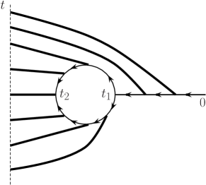
Figure 3: A generic one-loop diagram. The thick line represents the MF solution of the GF whose final time is $t$.

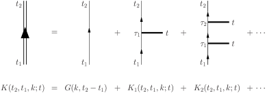
Figure 4: The one-particle Green function with insertions of trees.

where $t_{2}>t_{1}$ is assumed and

$$T(t)=(s-1)/(1+rt)$$ (41)

is the MF solution of the critical GF, i.e., $\bar{F}(s,t)$ at $\mu=0$ and $r=-(s-1)\alpha g/2$. Hence the sum over all tree insertions is

$$K(t_{2},t_{1},k;t)=\sum_{p=0}K_{p}(t_{2},t_{1},k;t)$$

$$=\theta(t_{2}-t_{1})\left(\frac{1+r(t-t_{2})}{1+r(t-t_{1})}\right)^{2}e^{-Dk^{2}(t_{2}-t_{1})}\ .$$ (42)

With the above Green function the sum over all one-loop diagrams has the form (see also Fig. 5).

$$L= -\frac{1}{2}\frac{g^{2}}{(8D\pi)^{d/2}}\int_{0}^{t}dt_{1}\int_{t_{1}}^{t}dt_{2}T(t-t_{2})$$

$$\times K^{2}(t_{2},t_{1},0;t)K(t_{1},0,0;t)(t_{2}-t_{1})^{-d/2}\ ,$$ (43)

where the integral over momentum was done.

Figure 5: The diagram of one-loop corrections to the GF. The thick line whose terminal point is $t$ is the MF GF and the double-line with arrow is the one-particle Green function with insertions of all trees.

The integrals in the foregoing expression are standard and we have, using dimensional regularization,

$$L =-\frac{u^{2}(s-1)}{(1+rt)^{2}}\left[-\frac{1}{1-\epsilon/2}\left(\frac{2}{\epsilon}\left(\frac{t}{\bar{t}}\right)^{\frac{\epsilon}{2}}+rt\left(\frac{t}{\bar{t}}\right)^{\frac{\epsilon}{2}}\right)\right.$$

$$-3\frac{2}{\epsilon}\frac{rt}{1+\epsilon/2}\left(\frac{t}{\bar{t}}\right)^{\frac{\epsilon}{2}}+3\frac{1}{1+\epsilon/2}\left(rt-\log(1+rt)\right)$$

$$\left.-\frac{1}{2+\epsilon/2}\left(2rt-2\log(1+rt)-\frac{r^{2}t^{2}}{1+rt}\right)+O(\epsilon)\right],$$ (44)

where $\epsilon=4-d$, $u=\sqrt{K_{4}}(g/D)\kappa^{-\epsilon/2}/4$ with $K_{4}=1/(8\pi^{2})$ is the dimensionless coupling constant, and ${\bar{t}}^{-1}=8\pi D\kappa^{2}$ with $\kappa^{-1}$ an arbitrary length scale. The renormalized GF can be obtained using the standard renormalization constants $Z_{\phi}=1+(2/\epsilon)u^{2}$ and $Z_{g}=1+(5/\epsilon)u^{2}$; see Eq. (16). Hence, the renormalized GF up to one-loop order is

$$\bar{F}(s,t) =\frac{(s-1)}{1+rt}\left[1+\frac{u^{2}}{1+rt}\biggl{(}1+\log(t/\bar{t})\right.$$

$$\left.+2\log(1+rt)+rt\biggl{(}3\log(t/\bar{t})-\frac{4+\frac{9}{2}rt}{1+rt}\biggr{)}\biggr{)}\right]\ .$$ (45)

For the calculation of the logarithmic correction we use the Wilson functions in two-loop order from Ref. Janssen (2000)

$$\beta(u) =6u^{3}-\frac{1}{4}\left(169+106\ln\frac{4}{3}\right)u^{5},$$ (46)

$$\gamma_{\phi}(u) =-2u^{2}+2\left(6-9\ln\frac{4}{3}\right)u^{4},$$ (47)

$$\gamma_{D}(u) =-u^{2}+\frac{1}{4}\left(17-2\ln\frac{4}{3}\right)u^{4},$$ (48)

with the observation that in Ref. Janssen (2000) the Wilson functions are written for the square of our coupling constant multiplied by a different factor.

The characteristic system to be solved is (see Eqs. (V-36))

$$\rho\frac{du}{d\rho} =\beta(u),$$ (49)

$$\rho\frac{d\alpha(\rho)}{d\rho} =(-2+\gamma_{\phi}(u)/2)\alpha(\rho),$$ (50)

$$\rho\frac{dt(\rho)}{d\rho} =(2+\gamma_{D}(u))t(\rho)\ .$$ (51)

Using $d\rho/\rho=dw/\beta(w)$, we have

$$t(w)=tC_{t}w^{a_{0}}\exp[-1/(\beta_{3}w^{2})+b_{0}w^{2}\!+O(w^{4})]\ ,$$ (52)

$$\alpha(w)=C_{\alpha}w^{a_{1}}\exp[1/(\beta_{3}w^{2})+b_{1}w^{2}+O(w^{4})]\ ,$$ (53)

$$\int_{u}^{w}\frac{\gamma_{\phi}(w^{\prime})}{\beta(w^{\prime})}dw^{\prime}=N^{\prime}w^{a_{2}}\exp[b_{2}w^{2}+O(w^{4})]\ ,$$ (54)

where $C_{t}$, $C_{\alpha}$ are determined from the initial condition $t(w=u)=t$, $\alpha(w=u)=\alpha$. We denote by $\beta_{i}$, $\phi_{i}$ and $D_{i}$ the coefficients in the expansion of the Wilson functions $\beta(w)$, $\gamma_{\phi}(w)$ and $\gamma_{D}(w)$ that generically can be written $Q=\sum_{i}c_{Q,i}u^{i}$, similar to the notations used in Ref. Janssen and Stenull (2004). The constants $a_{0}$, $a_{1}$, $a_{2}$, $b_{0}$, $b_{1}$, $b_{2}$ are defined by the following relations

$$a_{0} =\frac{1}{\beta_{3}^{2}}(D_{2}\beta_{3}-2\beta_{5})\ ,$$ (55)

$$a_{1} =\frac{1}{2\beta_{3}^{2}}(\phi_{2}\beta_{3}+4\beta_{5})\ ,$$ (56)

$$a_{2} =\phi_{2}/\beta_{3}\ ,$$ (57)

$$b_{0} =\frac{1}{2\beta_{3}^{2}}\left(D_{4}\beta_{3}-D_{2}\beta_{5}\right)+\frac{\beta_{5}^{2}}{\beta_{3}^{3}}\ ,$$ (58)

$$b_{1} =\frac{1}{4\beta_{3}^{2}}\left(\phi_{4}\beta_{3}-\phi_{2}\beta_{5}\right)-\frac{\beta_{5}^{2}}{\beta_{3}^{3}}\ ,$$ (59)

$$b_{2} =\frac{1}{2\beta_{3}^{2}}(\phi_{4}\beta_{3}-\phi_{2}\beta_{5})\ .$$ (60)

Under scaling the generating function transforms as follows:

$$\bar{F}(s,t;w,\alpha) =\exp\left[\int_{u}^{w}dw^{\prime}\gamma_{\phi}(w^{\prime})/\beta(w^{\prime})\right]$$

$$\times\bar{F}(s,t(w);w,\alpha(w))\ ,$$ (61)

where we can eliminate $w$ with the condition $t(w)=X_{0}\bar{t}$ with $X_{0}$ an arbitrary constant of order one. The GF at large $t$ is

$$\bar{F}(s,t) =\frac{N^{\prime}(s-1)w^{a_{2}}e^{b_{2}w^{2}+O(w^{4})}(1+(\ln X_{0}+1)w^{2})}{S(w,s,t)}\left[1+\frac{w^{2}}{S(w,s,t)}\biggr{(}1+\log X_{0}+2\log(S(w,s,t))\right.$$

$$\left.-(1-S(w,s,t))\left(3\log X_{0}-\frac{9}{2}+\frac{1}{2S(w,s,t)}\right)\biggr{)}\right]\ ,$$ (62)

where

$$S(w,s,t)=1-\frac{1}{2}(s-1)\bar{D}tw^{a_{0}+a_{1}+1}e^{(b_{0}+b_{1})w^{2}+O(w^{4})}\ ,$$ (63)

$\bar{D}=C_{\alpha}C_{t}DK_{4}^{-1/2}$ and for large $t$ we have from Eq. (52)

$$w =\tau^{-1/2}\exp\left[\frac{a_{0}\beta_{3}}{4}\frac{\ln\tau}{\tau}+O\left(\tau^{-2}\ln^{2}\tau\right)\right]\ ,$$ (64)

$$\tau =\beta_{3}\ln(t/t_{0})\ .$$ (65)

with $t_{0}=(X_{0}/C_{t})\bar{t}$.

References

- Hinrichsen (2000) H. Hinrichsen, Adv. Phys. 49, 815 (2000); and the references therein.
- (2) H. -K. Janssen, Z. Phys. B 42, 151 (1981).
- (3) P. Grassberger, Z. Phys. B 47, 365 (1982).
- (4) For a recent review, see M. Henkel and H. Hinrichsen, J. Phys. A 37, R117 (2004).
- (5) H.-K. Janssen, F. van Wijland, O. Deloubrir̀e, and U. C. Täuber, Phys. Rev. E 70, 056114 (2004).
- (6) S.-C. Park and H. Park, Phys. Rev. Lett. 94, 065701 (2005); Phys. Rev. E 71, 016137 (2005).
- Cardy and Täuber (1998) J. L. Cardy and U. C. Täuber, J. Stat. Phys. 90, 1 (1998).
- Cardy (1999) J. Cardy, Field theory and non-equilibrium statistical mechanics (unpublished).
- (9) U. C. Täuber, M. Howard, and B. P. Vollmayr-Lee, J. Phys. A 38, R79 (2005); and the references therein.
- (10) H.-K. Janssen and U. C. Täuber, Ann. Phys. (NY) 315, 147 (2005); cond-mat/0409670.
- Janssen (2000) H.-K. Janssen, J. Stat. Phys. 103, 801 (2001).
- (12) H.-K. Janssen, Ü. Kutbay, K. Oerding, J. Phys. A 32, 1809 (1999).
- (13) F. van Wijland, K. Oerding, and H. J. Hilhorst, Physica A 251, 179 (1998).
- Janssen and Stenull (2004) H.-K. Janssen and O. Stenull, Phys. Rev. E 69, 016125 (2004).
- Lübeck (2004) S. Lübeck, Int. J. Mod. Phys. B 18, 3977 (2004).
- Janssen (2003) H.-K. Janssen, J. Phys.: Condens. Matter 17, S1973 (2005); cond-mat/0304631.
- (17) M. Howard and C. Godrèche, J. Phys. A 31, L209 (1998).
- (18) D. J. Amit, Field theory, the Renormalization Group, and Critical Phenomena (World Scientific, Singapore, 1984); J. Zinn-Justin, Quantum Field Theory and Critical Phenomena (Claredon, Oxford, 1996).
- (19) D. Stauffer, M. Ferer, and M. Wortis, Phys. Rev. Lett. 29, 345 (1972).
- (20) S.-C. Park, cond-mat/0412749.
- (21) I. Jensen, J. Phys. A 32, 5233 (1999).
- (22) T.E. Harris, Ann. Prob. 2, 969 (1974).