How to calculate the main characteristics of random uncorrelated networks

Abstract

We present an analytic formalism describing structural properties of random uncorrelated networks with arbitrary degree distributions. The formalism allows to calculate the main network characteristics like: the position of the phase transition at which a giant component first forms, the mean component size below the phase transition, the size of the giant component and the average path length above the phase transition. We apply the approach to classical random graphs of Erdös and Rényi, single-scale networks with exponential degree distributions and scale-free networks with arbitrary scaling exponents and structural cut-offs. In all the cases we obtain a very good agreement between results of numerical simulations and our analytical predictions.

1 Introduction

During the last years, there has been noticed a significant interest in the field of complex networks and a lot of interdisciplinary initiatives have been taken aiming at investigations of these systems 0a ; 0b ; 1 ; 14 . It was observed that despite network diversity, most of real web-like systems share three prominent characteristics: small-world property (i.e. small average path length), high clustering and scale-free degree distribution 32 ; 22 . The observed universal properties let one understand that networks are not simply a sum of nodes connected by links. Nowadays, research on networks points mainly to the so-called emergent properties, that is systems global features and capabilities which are not specified by network design and are difficult or impossible to predict from knowledge of its constituents. As a result, the interest in topological characterization of real networks gives way to growing interest in dynamical processes defined on such systems BAfluct ; BianSOC . We have already known how networks grow and how that growth process influences network topology i.e. pattern of connections 12 ; VespPRL . We have also gained a certain understanding of how network structure mediates different transport phenomena like: disease (rumor) transmission in social networks NewEp or information processing (virus infection) in computer networks PastorEp . However, there is still a number of open question like: what are the most efficient and robust topologies for different web-like systems BANature ? How to effectively fight against criminal networks netwars ? How to eliminate traffic jams in the Internet and other transportation systems TadicPRE ?

This paper is devoted to uncorrelated random networks NewPRE (also known as random graphs or configuration model) which have been repeatedly shown to be very useful in modeling different phenomena taking place on networks. Although a number of other network models have been proposed, it was also proved that in many cases there are no qualitative differences between phenomena defined on both random graphs and those more sophisticated models. For example, the main results on percolation transition NewPRL1 ; NewPRL2 and epidemic spreading PastorEp ; BagunaPRL that were obtained for random uncorrelated networks are still valid for correlated and even non-equilibrium systems. The above certifies that despite its simplicity, configuration model is not merely mathematical toy. For the mentioned reasons, the issue of structural properties of random graphs and their reliable, mathematical description seems to be very important. It does not only excel in academic challenges but it can be helpful in further exploration of networks, including dynamical processes defined on discrete, web-like topologies.

Following the idea, in this paper we proceed with microscopic description of the considered networks and ask the most basic question related to their structural properties i.e. what is the probability that the shortest distance between two given nodes $i$ and $j$ is not longer than $x$. Basing on simple, intuitive arguments we derive the probability and apply it to calculate the main network characteristics like: the position of the phase transition at which a giant component first forms molloy1 ; HavPRLpc , the mean component size below the phase transition NewPRE , the size of the giant component molloy2 ; NewPRL1 and the average path length above the phase transition DorMetric . Although most of the enumerated macroscopic properties were previously calculated by means of other methods, especially thanks to generating function formalism developed by Newman NewPRE , we think that our approach is conceptually much simpler. Furthermore, since our derivations take advantage of primary concepts they do not represent a closed project but can be thought of as a background for further network investigations, particularly those associated with network dynamics.

2 Random uncorrelated networks - microscopic description

Random uncorrelated network with arbitrary degree distribution $P(k)$ is the simplest network model. In such a network the total number of vertices $N$ is fixed. Degrees of all vertices are independent, random integers drawn from a specified distribution $P(k)$. One can easily create the network following the below instructions:

• Prepare $N$ nodes $i=1,2,\dots,N$.

• Attach to each node $k_{i}$ ends of connections taken from the given distribution $P(k)$.

• Connect at random ends of connections.

The above procedure provides maximally random, uncorrelated networks. From the mathematical point of view the lack of correlations means that the probability $P(k_{i}/k_{j})$ that an edge departing from a vertex $j$ of degree $k_{j}$ arrives at a vertex $i$ of degree $k_{i}$, is independent of the initial vertex $j$. The above translates into the fact that the nearest neighborhood of each node is the same (in statistical terms). Provided that the degree distribution in uncorrelated network is $P(k)$ one can show that the degree distribution of nearest neighbors, that is equivalent to the probability that an arbitrary link leads to a node $i$ of degree $k_{i}$, is given by

$$P(k_{i}/k_{j})=Q(k_{i})=\frac{k_{i}}{\langle k\rangle}P(k_{i}),$$ (1)

and respectively the average nearest neighbor degree equals

$$\langle k_{nn}\rangle=\frac{\langle k^{2}\rangle}{\langle k\rangle}.$$ (2)

At the moment, before we proceed with our derivations, let us introduce notation that will be used throughout the paper:

• $p^{+}_{ij}(x)$ denotes the probability that there exists at least one walk of length $x$ between two given nodes $i$ and $j$. If such a walk exists then the shortest path between the two nodes is $\leq x$.

• $p^{-}_{ij}(x)$ gives the probability that none among walks of length $x$ occurs between the two nodes, and respectively

  $$p^{-}_{ij}(x)=1-p^{+}_{ij}(x).$$ (3)

• $p^{*}_{ij}(x)$ describes the probability that the shortest distance between $i$ and $j$ is equal to $x$. In the limit of dense networks (above percolation threshold) one can deduce that if there exists at least one walk of length $x$ between $i$ and $j$ then walks longer than $x$ also exist. It follows, one can assume that $p_{ij}^{+}(x)$ (see i.) expresses also the probability that the shortest distance between the two nodes is not longer than $x$ and

  $$p^{*}_{ij}(x)=p^{+}_{ij}(x)-p^{+}_{ij}(x-1).$$ (4)

Now, we try to derive formulas describing the above probabilities. At the beginning, let us imagine a random walker that starts at a given node $i$ and assign the walker one-step memory in order to avoid backward steps. Next, let the walker perform $x$ steps. It is easy to see that in average the walker may pass

$$W(i,x)=k_{i}(\langle k_{nn}\rangle-1)^{x-1}$$ (5)

different walks. If, at least one such a walk ends at the node $j$ one can say that both vertices $i$ and $j$ are at most $x-$th neighbors i.e. the shortest path between the two nodes is not longer than $x$. It follows that

$$p^{+}_{ij}(x)=P\left(\bigcup_{r=1}^{W(i,x)}W^{(r)}_{i\rightarrow j}\right),$$ (6)

where $W^{(r)}_{i\rightarrow j}$ represents a single walk between $i$ and $j$, whereas the sum goes over all possible $x-$walks starting at $i$ (5).

To simplify the last expression (6) let us assume mutual independence of all walks $W^{(r)}_{i\rightarrow j}$. Then, the considered formula may be rewritten in the following form (see Appendix A)

$$p^{+}_{ij}(x)\simeq 1-\exp\left[-\sum_{r=1}^{W(i,x)}P\left(W^{(r)}_{i\rightarrow j}\right)\right].$$ (7)

To finalize derivation of $p^{+}_{ij}(x)$ note that, due to the lack of correlations, every walk starting at $i$ has the same chance to end up in $j$. The probability of such an event is just equal to the probability that the last connection in the sequence of edges representing the considered walk is attached to $j$

$$P\left(W^{(r)}_{i\rightarrow j}\right)=\frac{k_{j}}{\langle k\rangle N}.$$ (8)

Inserting the last formula into (7) and taking advantage of both (5) and (2) one gets

$$p^{+}_{ij}(x)=1-F(x),$$ (9)

where

$$F(x)=\exp\left[-\frac{k_{i}k_{j}}{\langle k\rangle N}\left(\frac{\langle k^{2}\rangle}{\langle k\rangle}-1\right)^{x-1}\right].$$ (10)

The last formula for $p^{+}_{ij}(x)$ constitutes the most important result of the paper. Let us stress that it does not include any free parameters, therefore one can directly employ it to calculate all the interesting structural characteristics of the considered networks. In the following sections we show, how the formula for percolation threshold in random graphs several times naturally emerges from our approach. We also calculate, in turn, the mean component size below the percolation transition, the size of the giant component and also the average path length above this transition.

3 Mean component size below percolation threshold

To calculate the mean component size below the percolation threshold one can make use of the introduced probabilities $p^{+}_{ij}(x)$ and $p^{-}_{ij}(x)$.

Taking advantage of (9), the probability that none among the walks of length $x$ between the nodes $i$ and $j$ exists is given by (3)

$$p_{ij}^{-}(x)=\exp\left[-\frac{k_{i}k_{j}}{\langle k\rangle N}\left(\frac{\langle k^{2}\rangle}{\langle k\rangle}-1\right)^{x-1}\right],$$ (11)

and respectively the probability that there is no walk of any length between these vertices may be written as

$$P_{ij}^{-}=\prod_{x=1}^{\infty}p_{ij}^{-}(x)=\exp\left[-\frac{k_{i}k_{j}}{\langle k\rangle N}\sum_{y=0}^{\infty}\left(\frac{\langle k^{2}\rangle}{\langle k\rangle}-1\right)^{y}\right].$$ (12)

The value of $P_{ij}^{-}$ strongly depends on the common ratio of the geometric series present in the last equation. When the common ratio is greater then $1$, i.e. $\langle k^{2}\rangle\geq 2\langle k\rangle$, random graphs are above the percolation threshold. The sum of the geometric series in (12) tends to infinity and $P_{ij}^{-}=0$. Below the phase transition, when $\langle k^{2}\rangle<2\langle k\rangle$, the probability that the nodes $i$ and $j$ belong to separate clusters is given by

$$P_{ij}^{-}=\exp\left[-\frac{k_{i}k_{j}}{N}\frac{1}{(2\langle k\rangle-\langle k^{2}\rangle)}\right],$$ (13)

and respectively the probability that $i$ and $j$ belong to the same cluster may be written as

$$P_{ij}^{+}=1-P_{ij}^{-}=1-\exp\left[-\frac{k_{i}k_{j}}{N}\frac{1}{(2\langle k\rangle-\langle k^{2}\rangle)}\right].$$ (14)

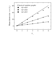
Figure 1: Average size of the component that a node of degree $k$ belongs to. Scatter plots represent numerical data, whereas solid lines represent the prediction of Eq. (15).

Now, it is simple to calculate the mean size of the cluster that the node $i$ belongs to. It is given by

$$\langle s\rangle(k_{i})=1+\sum_{k_{j}}P(k_{j})P_{ij}^{+}\simeq\frac{\langle k\rangle}{2\langle k\rangle-\langle k^{2}\rangle}k_{i}+1.$$ (15)

Note, that the mean size of the component that a node $i$ belongs to, is a linear function of degree $k_{i}$ of the node (see Fig. 1). The last transformation in (15) was obtained by taking only the first two terms of power series expansion of the exponential function in (14). Averaging the above expression (15) over all nodes in the network one obtains the known formula NewPRE for the mean component size in random graphs below the phase transition

$$\langle s\rangle=1+\frac{\langle k\rangle^{2}}{2\langle k\rangle-\langle k^{2}\rangle}.$$ (16)

As in percolation theory Stauffer , the mean cluster size diverges at

$$\langle k^{2}\rangle=2\langle k\rangle,$$ (17)

one more time certifying that the expression (17) describes the position of the percolation threshold in random uncorrelated networks with arbitrary degree distributions molloy1 ; HavPRLpc .

4 Size of the giant component

When $\langle k^{2}\rangle>2\langle k\rangle$ the giant component (GC) is present in the graph. Its relative size $S$, i.e. the probability that a node belongs to GC, is an important quantity and is often identified as the order parameter of the percolation transition. In this section, we demonstrate how to calculate the size of the giant component $S$ in uncorrelated networks with arbitrary degree distributions. The underlying concept of our derivations is closely related to the method of calculating $S$ in Cayley tree and originates from Flory (1941) Flory ; Stauffer .

At the beginning, we deal with classical random graphs of Erdös and Rényi, then we generalize our calculations for the case of random graphs with arbitrary degree distributions and we show that our derivations are consistent with the formalism based on generating functions that was introduced by Newman et al. NewPRE .

4.1 Classical random graphs of Erdös and Rényi (ER)

In general, one defines the classical random graph as N labeled nodes and every pair of the nodes being connected with probability $p$ Bollobas . The probability that an arbitrary node $i$ belongs to the giant component is equivalent to the probability that at least one of its $N-1$ possible links connects it to GC. In order to describe the above equivalence by means of mathematical expression, let us assume that $A_{\{i,j\}}$ represents an event: the connection $\{i,j\}$ (if exists!) leads to the giant component. The notation $A_{\{i,j\}}$ refers to each of $N(N-1)/2$ possible links, not only to those existing! Now, the size of the giant component is given by

$$S=P\left(\bigcup_{j=1}^{N-1}A_{\{i,j\}}\right),$$ (18)

and due to the mutual independence of different links, the last formula may be rewritten as (see Appendix A)

$$S=1-\exp\left[-\sum_{j=1}^{N-1}P(A_{\{i,j\}})\right].$$ (19)

Next, to further simplify the expression for $S$ note that the mentioned mutual independence implies that every link has the same probability to belong to the infinite cluster i.e.

$$\forall_{\{i,j\}}\;\;P(A_{\{i,j\}})=R.$$ (20)

Inserting (20) into (19) one gets

$$S=1-\exp[-(N-1)R].$$ (21)

To finalize derivation of $S$ one has to find $R$. To do so, let us recall that $R$ describes the probability that an arbitrary node $i$ is connected to the giant component through a fixed link $\{i,j\}$, where $j$ is another arbitrary node. Now, if $j$ belongs to GC it means that at least one of its connections also leads to the giant component. Given that every node may have $N-1$ links the formula for $R$ may be expressed as a product of the probability of a link $\{i,j\}$ and the probability that at least one of $N-1$ possible links emanating from $j$ connects the considered node to the giant component. Summarizing the above considerations one obtains a self-consistency equation for $R$

$$R=P(A_{\{i,j\}})=pP\left(\bigcup_{m=1}^{N-1}A_{\{j,m\}}\right)$$ (22)

$$=p(1-\exp[-(N-1)R]).\;$$

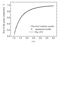
Figure 2: Size of the giant component $S$ versus the average degree $\langle k\rangle$ in classical random graphs of size $N=10000$. The scatter plot represents numerical data whereas the solid line gives the solution of the Eq. (23)

.

Finally, comparing both relations (21) and (22) it is easy to see that $R=pS$ and the expression for the giant component in classical random graphs may be rewritten in the following form molloy2

$$S=1-\exp[-\langle k\rangle S],$$ (23)

where $\langle k\rangle=pN$ (see Fig. 2). At the moment let us point a certain interesting property of the last equation, that makes the equation very intuitive example of percolation transition (at least for those acquainted with Ising model). Below the percolation threshold (i.e. for $\langle k\rangle<1$ ) the identity has only one solution $S=0$ (see Fig. 3). Above the threshold another solution $S\neq 0$ appears signifying transition of the system to the ordered phase.

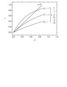
Figure 3: Graphical solution of the Eq. (23).

4.2 Giant component in random graphs with arbitrary degree distributions

In this section, taking advantage of the intuition gained from the analysis of the giant component in classical random graphs, we develop a more general approach allowing to calculate the size of the giant cluster in random networks with arbitrary degree distributions $P(k)$.

In the case of classical random graphs all nodes have been considered equivalent. It is not acceptable in the case of random graphs with a given degree sequence $P(k)$, where every node has a fixed number of connections. In order to meet the requirements imposed by $P(k)$, we have to slightly rearrange the previous meaning of the probability $R$ (20). Now, let us assume that $R$ describes the probability that an arbitrary but existing (!) connection belongs to the giant component. It is also useful to think of $R$ as the probability that following arbitrary direction of a randomly chosen edge one arrives at the giant component. In fact, we know that following an arbitrary edge we arrive at a vertex of degree $k$. The probability that the node, we have just arrived at, is connected to GC equals $1-(1-R)^{k-1}$. The last relation simply expresses the probability that at least one of $k-1$ edges emanating from $i$ and other than the edge we arrived along connects $i$ to the giant component . Summarizing the above considerations makes simple to write the self-consistency condition for $R$ (compare with Eq. (22))

$$R=\sum_{k}\left(1-(1-R)^{k-1}\right)Q(k),$$ (24)

where $Q(k)$ is given by (1). Then, knowing $R$ it is easy to calculate the relative size $S$ of the giant component that is equivalent to the probability that at least one of $k$ links attached to an arbitrary node connects the node to GC

$$S=\sum_{k}\left(1-(1-R)^{k}\right)P(k).$$ (25)

To make derivations of this section more concrete, we should immediately introduce some examples of specific networks. Since however, one can show that both formulas (25) and (24) are completely equivalent to equations derived by other authors (see Appendix B), we just refer the reader to analyze examples presented in those related papers NewPRE ; NewSIAM .

5 Average path length in random uncorrelated networks

We turn now to the quantitative description of the small-world effect in random uncorrelated networks with arbitrary degree distributions $P(k)$. To our knowledge, the below derivations are the simplest and the most accurate among those previously reported NewPRE ; MotterPRE ; DorMetric , therefore we illustrate them with a larger number of examples.

Taking advantage of (9), we are in a position to calculate $p_{ij}^{*}(x)$ (4) i.e. probability distribution for the shortest distance between any two nodes $i$ and $j$

$$p_{ij}^{*}(x)=F(x-1)-F(x),$$ (26)

where $F(x)$ is given by (10). Although, due to the condition $p_{ij}^{*}(x)\geq 0$ the last expression is only correct above the percolation threshold, the formula (26) is very important and, given that the giant component contains almost all vertices, it allows to find a number of structural properties of the considered networks. For example, averaging (26) over all pairs of nodes one obtains the intervertex distance distribution $p(x)=\langle\langle p_{ij}^{*}(x)\rangle_{i}\rangle_{j}$. It is also possible to calculate $z_{x}$ i.e. the mean number of vertices a certain distance $x$ away from a randomly chosen node $i$. The quantity can be obtained as $z_{x}=N\int p_{ij}^{*}(x)P(k_{j})dk_{j}$. At the moment, let us note that taking only the first two terms of power series expansion of both exponential functions $F$ in (26) one gets the relationship $z_{x}=z_{1}(z_{2}/z_{1})^{x-1}=\langle k\rangle(\langle k_{nn}\rangle-1)^{x-1}$ (compare it with (5)) that was obtained by other authors given the assumption of a tree-like structure of random graphs. Finally, the average path length (APL) between any two nodes $i$ and $j$ of degrees $k_{i}$ and $k_{j}$ is simply the expectation value of the distribution (26)

$$l_{ij}(k_{i},k_{j})=\sum_{x=1}^{\infty}xp_{ij}^{*}(x)=\sum_{x=0}^{\infty}F(x).$$ (27)

The Poisson summation formula allows one to simplify the above sum (see Appendix C)

$$l_{ij}(k_{i},k_{j})=\frac{-\ln(k_{i}k_{j})+\ln(\langle k^{2}\rangle-\langle k\rangle)+\ln N-\gamma}{\ln(\langle k^{2}\rangle/\langle k\rangle-1)}+\frac{1}{2},$$ (28)

where $\gamma\simeq 0.5772$ is the Euler’s constant. The average intervertex distance for the whole network depends on a specified degree distribution $P(k)$

$$l=\frac{-2\langle\ln k\rangle+\ln(\langle k^{2}\rangle-\langle k\rangle)+\ln N-\gamma}{\ln(\langle k^{2}\rangle/\langle k\rangle-1)}+\frac{1}{2}.$$ (29)

As one could expect, the both formulas (28) and (29) diverge when the considered networks approach percolation threshold $\langle k^{2}\rangle=2\langle k\rangle$ (17).

To test the formula (29) we have performed numerical simulations of the well-known networks: classical random graphs proposed by Erdös and Rényi (ER), single-scale networks with exponential degree distribution (EXP) and scale-free networks (SF).

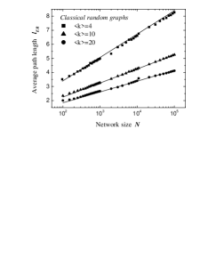
Figure 4: Average path length $l_{ER}$ versus network size $N$ in $ER$ classical random graphs with $\langle k\rangle=pN=4,10,20$. The solid curves represent numerical prediction of Eq. (31).

Classical random graphs (ER). For these networks the degree distribution is Poissonian

$$P(k)=\frac{e^{-\langle k\rangle}\langle k\rangle^{k}}{k!}.$$ (30)

However, since $\langle\ln k\rangle$ cannot be calculated analytically for Poisson distribution thus the $APL$ may not be directly obtained from (29). To overcome this problem we take advantage of the mean field approximation and assume that all vertices within a graph possess the same degree $\forall_{i}\>k_{i}=\langle k\rangle$. It implies that the $APL$ between two arbitrary nodes $i$ and $j$ (28) also describes the average intervertex distance characterizing the whole network

$$l_{ER}=\frac{\ln N-\gamma}{\ln(pN)}+\frac{1}{2}.$$ (31)

Until now only a rough estimation of the quantity has been known. One has expected that the average shortest path length of the whole ER graph scales with the number of nodes in the same way as the network diameter. We remind that the diameter $d$ of a graph is defined as the maximal distance between any pair of vertices and $d_{ER}=\ln N/\ln(pN)$ 1 . Figure 4 presents the prediction of the equation (31) in comparison with the numerically calculated APL in classical random graphs.

Figure 5: Characteristic path length $l_{EXP}$ versus network size $N$ in exponential networks. Solid lines represent Eq. (33).

Exponential networks (EXP). Now, let us suppose that the degree distribution is exponential

$$P(k)=\frac{e^{(1-k)/a}}{a},$$ (32)

where $k=1,2,\dots$ . Applying the distribution to Eq. (29) immediately provides the formula for the average path length in the considered single-scale networks

$$l_{EXP}=\frac{\ln N+\ln(2a^{2}+a)-2e^{1/a}\Gamma(0,1/a)-\gamma}{\ln(2a^{2}+a)-\ln(a+1)}+\frac{1}{2},$$ (33)

where $\Gamma(0,1/a)$ is an incomplete gamma function. Figure 5 shows that the obtained formula perfectly fits numerical results obtained for different values of the parameter $a$.

Scale-free networks (SF). As mention at the beginning of the paper degree distributions are scale-free in most of real systems

$$P(k)=\frac{(\alpha-1)m^{(\alpha-1)}}{k^{\alpha}},$$ (34)

where $k=m,m+1,\dots,k_{max}$. It was found that the most generic mechanism driving real networks into scale-free structures is the linear preferential attachment. The simplest model that incorporates the rule of preferential attachment was introduced by Barabási and Albert 22 . Other interesting mechanisms leading to scale-free networks were proposed by Goh et al. gohPRL2001 and Caldarelli et al. calPRL2002 . Unfortunately, the mentioned mechanisms leading to scale-free network topologies incorporate structural correlations, making our approach useless. The simple procedure of generating random uncorrelated networks that was described at the beginning of this paper also fails when applied to fat-tailed degree distributions with diverging second moment $\langle k^{2}\rangle$. In particular, the procedure may not be applied to generate uncorrelated scale-free networks (34) with the scaling exponent $2<\alpha<3$. In order to avoid the inconvenience connected with those scale-free distributions we apply the so-called structural cutoffs by imposing the largest degree to scale as $k_{max}=\sqrt{\langle k\rangle N}$ BurdaPRE ; BogunaEPJB ; CatanzaroPRE , instead of unbounded cutoff predicted by extreme value theory $k_{max}\sim N^{1/(\alpha-1)}$.

We have found that depending on the value of the exponent $\alpha$ one can distinguish three scaling regions for the average path length (29) in scale-free networks (see Fig. 6). In the limit of large systems $N\rightarrow\infty$, $APL$ scales according to relations

• for $\alpha>3$

  $$l^{\alpha>3}\sim\ln N,$$ (35)

• for $\alpha=3$

  $$l^{\alpha=3}\sim\frac{\ln N}{\ln\ln N},$$ (36)

• for $2<\alpha<3$

  $$l^{\alpha<3}=const.$$ (37)

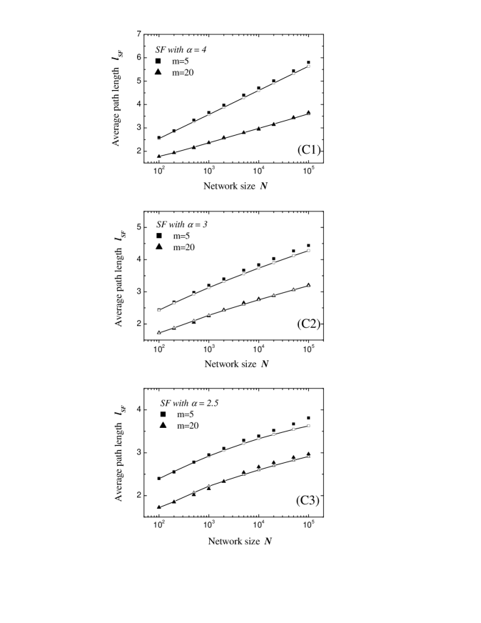
Figure 6: Average path length versus number of nodes $N$ in scale-free networks with $\alpha=4$ (C1), $\alpha=3$ (C2) and $\alpha=2.5$ (C3). The scatter data represent numerical calculations. Solid curves with open symbols express analytical predictions of Eq. (31).

Note that although the results for $\alpha\geq 3$ are consistent with estimations obtained by other authors DorMetric ; HavPRLultra , the case of $2<\alpha<3$ is different. In opposite to previous estimations signaling the double logarithmic dependence $l^{\alpha<3}\sim\ln\ln N$, our calculations for the same range of $\alpha$ predict that there is a saturation effect for the mean path length in large networks. Unfortunately, at the moment it is impossible to assess what is the correct estimation (to perform reliable tests very large networks, even with $N>10^{10}$, should be analyzed). On the other hand, it is truth that looking at Figure 6 one can observe two effects: i. the difference between results of numerical calculations and our analytical predictions continuously grows with $N$, ii. denser networks are better described by our approach. The first effect may result form the fact that our mean-field derivations work worse for networks with degree distributions characterized by large fluctuations (note that the second moment of scale-free distribution described by the exponent $\alpha\leq 3$ increases with $N$), whereas the second effect may be related to the fact that our approach (in particular Eq. (26)) works better for networks further above the percolation threshold

6 Conclusions

To conclude, in this paper we have presented theoretical approach for metric properties of uncorrelated random networks with arbitrary degree distributions. We have derived a formula for probability $p^{+}_{ij}(x)$ (9) that there exists at least one walk of length $x$ between two arbitrary nodes $i$ and $j$. We have shown that given $p^{+}_{ij}(x)$ one can find a number of structural characteristics of the studied networks. In particular, we have applied our approach to calculate the mean component size below the percolation transition, the size of the giant component and the average path length above the phase transition. We have successfully applied our formalism to such diverse networks like classical random graphs of Erdös and Rényi, single-scale networks with exponential degree distributions and uncorrelated scale-free networks with structural cut-offs. In all the studied cases we noticed a very good agreement between our theoretical predictions and results of numerical investigation.

7 Appendices

7.1 Appendix A

Lemma 1

If $A_{1},A_{2},\dots,A_{n}$ are mutually independent events and their probabilities fulfill relations $\forall_{i}P(A_{i})\leq\varepsilon$ then

$$P(\bigcup_{i=1}^{n}A_{i})=1-\exp(-\sum_{i=1}^{n}P(A_{i}))-Q,$$ (38)

where $0\leq Q<\sum_{j=0}^{n+1}(n\varepsilon)^{j}/j!-(1+\varepsilon)^{n}$.

Proof. Using the method of inclusion and exclusion Feller we get

$$P(\bigcup_{i=1}^{n}A_{i})=\sum_{j=1}^{n}(-1)^{j+1}S(j),$$ (39)

with

$$S(j)=\sum_{1\leq i_{1}<i_{2}<\dots<i_{j}\leq n}^{n}P(A_{i_{1}})P(A_{i_{2}})\dots P(A_{i_{j}})$$

$$=\frac{1}{j!}\left(\sum_{i=1}^{n}P(A_{i})\right)^{j}-Q_{j},$$ (40)

where $0\leq Q_{j}\leq\left(n^{j}/j!-\left({}^{n}_{j}\right)\right)\varepsilon^{j}$. The term in bracket represents the total number of redundant components occurring in the last line of (7.1). Neglecting $Q_{j}$ it is easy to see that $(1-P(\cup A_{i}))$ corresponds to the first $(n+1)$ terms in the MacLaurin expansion of $\exp(-\sum P(A_{i}))$. The effect of higher-order terms in this expansion is smaller than $R<(n\varepsilon)^{n+1}/(n+1)!$. It follows that the total error of (38) may be estimated as $Q<\sum_{j=1}^{n}Q_{j}+R$. This completes the proof.

Let us notice that the terms $Q_{j}$ in (7.1) disappear when one approximates multiple sums $\sum_{1\leq i_{1}<i_{2}<\dots<i_{j}\leq n}^{n}$ by corresponding multiple integrals. For $\varepsilon=A/n\ll 1$ the error of the above assessment is less then $A^{2}\exp(A)/n$ and may be dropped in the limit $n\rightarrow\infty$.

7.2 Appendix B

It is easy to show that our formulas (25) and (24) are completely equivalent to equations derived by Newman et al. NewPRE by means of generating functions

$$S=1-G_{0}(v),$$ (41)

where $v$ is the solution of equation given below

$$v=G_{1}(v).$$ (42)

We recall that $G_{0}(x)$ is the generating function for the degree distribution

$$G_{0}(x)=\sum_{k}P(k)x^{k},$$ (43)

whereas $G_{1}(x)$ is related to $Q(k)$ (1)

$$G_{1}(x)=\frac{1}{\langle k\rangle}\frac{dG_{0}(x)}{dx}=\sum_{k}Q(k)x^{k-1}.$$ (44)

Let us start with Eq. (24) that may be transformed in the following way

$$R=\sum_{k}Q(k)-\sum_{k}Q(k)(1-R)^{k-1}=1-G_{1}(1-R).$$ (45)

Note, that the last formula directly corresponds to Eq. (42) with

$$v=1-R.$$ (46)

Taking into account the last identity one can show that the expression (25) may be transformed into Eq. (41) in a similar way. Now, it is clear that the unknown parameter $v$ in both Eqs. (41) and (42) has the following meaning - it describes the probability that an arbitrary edge in a random graph does not belong to the giant component.

7.3 Appendix C

The Poisson summation formula states

$$\sum_{x=0}^{\infty}F(x)=\frac{1}{2}F(0)+\;\;\;\;\;\;\;\;\;\;\;\;\;\;\;\;\;\;\;\;\;\;\;\;\;\;\;\;\;\;\;\;\;\;\;\;\;\;\;\;\;\;\;\;\;\;\;\;\;\;\;\;\;\;$$ (47)

$$\;\;\;\;\;\;\;\;\;\;\;\;\;\;\;\int_{0}^{\infty}F(x)dx+2\sum_{n=1}^{\infty}\left(\int_{0}^{\infty}F(x)\cos(2n\pi x)dx\right).$$

Applying the formula to (28)

$$l_{ij}(k_{i},k_{j})=\sum_{x=0}^{\infty}\exp\left[-\frac{k_{i}k_{j}}{(\langle k^{2}\rangle-\langle k\rangle)N}\left(\frac{\langle k^{2}\rangle}{\langle k\rangle}-1\right)^{x\;}\right]$$ (48)

one realizes that in most of cases

$$\frac{k_{i}k_{j}}{(\langle k^{2}\rangle-\langle k\rangle)N}\simeq 0$$ (49)

that gives $F(0)=1$. One can also find that

$$\int_{0}^{\infty}F(x)dx=-Ei\left(-\frac{k_{i}k_{j}}{(\langle k^{2}\rangle-\langle k\rangle)N}\right)/\ln\left(\frac{\langle k^{2}\rangle}{\langle k\rangle}-1\right),$$ (50)

where $Ei(y)$ is the exponential integral function that for negative arguments is given by $Ei(-y)=\gamma+\ln y$ Ryzyk , where $\gamma\simeq 0.5772$ is the Euler’s constant. Finally, it is easy to see that owing to the generalized mean value theorem every integral in the last term of the summation formula (47) is equal to zero. It follows that the equation for $l_{ij}(k_{i},k_{j})$ is given by (28).

References

- (1) S. Bornholdt and H.G. Schuster, Handbook of Graphs and networks, Wiley-Vch (2002).
- (2) S.N. Dorogovtsev and J.F.F. Mendes, Evolution of Networks, Oxford Univ.Press (2003).
- (3) R. Albert and A.L. Barabási, Rev. Mod. Phys. 74, 47 (2002).
- (4) S.H. Strogatz, Nature 410, 268 (2001).
- (5) D.J. Watts and S.H. Strogatz, Nature 393, 440 (1998).
- (6) A.L. Barabási and R. Albert, Science 286, 509 (1999).
- (7) M. Argollo de Menezes and A.L. Barabási, Phys. Rev. Lett. 92, 028701 (2004).
- (8) G. Bianconi and M. Marsili, Phys. Rev. E 70, 035105(R) (2004).
- (9) S.N. Dorogovtsev et al., Phys. Rev. Lett. 85, 4633 (2000).
- (10) A. Barrat et al., Phys. Rev. Lett. 92, 228701 (2004).
- (11) M.E.J. Newman, Phys. Rev. Lett. 66, 016128 (2002).
- (12) R. Pastor-Satorras and A. Vespignani, Phys. Rev. Lett. 86, 3200 (2001).
- (13) R. Albert et al., Nature 406, 378 (2000).
- (14) V.E. Krebs, Connections 24(3), 43 (2001).
- (15) B. Tadić et al., Phys. Rev. E 69, 036102 (2004).
- (16) M.E.J. Newman et al., Phys. Rev. E 64, 026118 (2001).
- (17) D.S. Callaway et al., Phys. Rev. Lett. 85, 5468 (2002).
- (18) M.E.J. Newman et al., Phys. Rev. Lett. 89, 208701 (2002).
- (19) M. Boguñá et al., Phys. Rev. Lett. 90, 028701 (2003).
- (20) M. Molloy and B. Reed, Ran. Struct. and Algor. 6, 161 (1995).
- (21) R. Cohen et al., Phys. Rev. Lett. 85, 4626 (2000).
- (22) M. Molloy and B. Reed, Combinatorics, Probab. Comput. 7, 295 (1998).
- (23) S.N. Dorogovtsev et al., Nucl. Phys. B 653, 307 (2003).
- (24) D. Stauffer and A. Aharony, Introduction to Percolation Theory, Taylor and Francis, London (1994).
- (25) P.J. Flory, J. Amer. Chem. Soc. 63, 3083 (1941).
- (26) B. Bollobás, Random graphs, Academic Press, New York (1985).
- (27) M.E.J. Newman, SIAM Review 45, 167 (2003).
- (28) A.E. Motter et al., Phys. Rev. E 66, 065103(R) (2002).
- (29) K.-I. Goh et al., Phys. Rev. Lett. 87, 278701 (2001).
- (30) G. Caldarelli et al., Phys. Rev. Lett. 89, 258702 (2002).
- (31) Z. Burda and A. Krzywicki, Phys. Rev. E 67, 046118 (2003).
- (32) M. Boguñá et al., Euro. Phys. J. B 38, 205 (2004).
- (33) M. Catanzaro et al., cond-mat/0408110 (2004).
- (34) R. Cohen and S. Havlin, Phys. Rev. Lett. 90, 058701 (2003).
- (35) W. Feller, An Introduction to Probability Theory and its Applications, John Wiley and Sons (1968).
- (36) I.S. Gradshteyn et al., Table of Integrals, Series, and Products, Academic Press (2000).
- (37) R.J. Wilson, Introduction to Graph Theory, Longman (1985).