Quantum Charge Fluctuations in a Superconducting Grain

Abstract

We consider charge quantization in a small superconducting grain that is contacted by a normal-metal electrode and is controlled by a capacitively coupled gate. At zero temperature and zero conductance $G$ between the grain and the electrode, the charge $Q$ as a function of the gate voltage $V_{g}$ changes in steps. The step height is $e$ if $\Delta<E_{c}$, where $\Delta$ and $E_{c}$ are, respectively, the superconducting gap and the charging energy of the grain. Quantum charge fluctuations at finite conductance remove the discontinuity in the dependence of $Q$ on $V_{g}$ and lead to a finite step width $\propto G^{2}\Delta$. The resulting shape of the Coulomb blockade staircase is of a novel type. The grain charge is a continuous function of $V_{g}$ while the differential capacitance, $dQ/dV_{g}$, has discontinuities at certain values of the gate voltage. We determine analytically the shape of the Coulomb blockade staircase also at non-zero temperatures.

I Introduction

In the conditions of Coulomb blockade, the charge of a grain is well-defined and discrete. It can be varied by means of the external parameter, gate voltage $V_{g}$. Periodically in $V_{g}$, the ground state of the system approaches a point of degeneracy, in which two consecutive allowed values of charge yield the same energy of the ground state. In the limit of no tunneling between the grain and particle reservoirs (leads), the degeneracy between the ground states is indeed reached at the corresponding special values of $V_{g}$. However, electron tunneling between the grain and leads may remove the degeneracy. The nature of the resulting many-body ground state is sensitive to the spectrum of excitations in the grain and in the leads. Except for the case of ultra-small grains,vonDelftO1 the level spacing between the single-particle excitations $\delta$ in metallic grains is usually negligible. Under this condition, there are the following three known types of evolution of the ground state with the variation of the external parameter $V_{g}$.

If the grain and leads are normal metals (N-I-N junction) the system at the charge degeneracy point can be mapped on the multi-channel Kondo problem.Matveev91 In this mapping, two subsequent values of charge and the gate voltage play the role of the pseudo-spin and magnetic field, respectively. (Normal grain charging was experimentally studied in Ref. Lehnert, .) Similar mapping is also possibleZaikin for a system consisting of a normal lead and a superconducting grain (S-I-N junction) in the case of relatively small charging energy $E_{c}<\Delta$ ($\Delta$ is the superconducting gap in the spectrum of excitations); tunneling then lifts the degeneracy between two states with charges differing by $2e$. The corresponding $2e$ steps in the grain charge were observed experimentally,Lafarge93b ; Lafarge93a but there was no detailed study of the charge dependence on $V_{g}$ near the degeneracy point.

In the opposite case of a fully superconducting system (S-I-S junction) with $E_{c}<\Delta$, the degeneracy removal is equivalent to the formation of an avoided crossing in a two-level system. Charge degeneracy for such junctions was studied experimentally.Schoelkopf

The third and the last out of the studied classes of junctions is represented by a system consisting of a normal grain and a superconducting lead (N-I-S junction), in which case the degeneracy is not removed by tunneling. Indeed, the ground state is degenerate with respect to changing the number of electrons in the grain by one, whereas the particle reservoir may supply only pairs of electrons.Matveev1998

We demonstrate here the existence of a new class of behavior of the ground state. It occurs in an S-I-N junction having normal lead made of a metal and characterized by charging energy $E_{c}>\Delta$. An adequate model for such a junction has large number of channels. We show that in the limit of infinite number of channels, the dependence of charge $Q$ on $V_{g}$ has no discontinuities, but the corresponding differential capacitance, $C_{\text{diff}}=dQ/dV_{g}$, remains singular, exhibiting a jump at some value of $V_{g}$. We find the full dependence $Q(V_{g})$ at a finite (but small, $G\ll 4\pi e^{2}/\hbar$) conductance. The smearing of the steps in $Q(V_{g})$ due to quantum fluctuations may be observed in experiments of the type performed in Refs. Lafarge93b, and Lafarge93a, at higher values of the junction conductance, or by using the sensitive charge measuring techniques of Ref. Lehnert, . We also find the evolution of the $Q(V_{g})$ dependence with temperature, and find conditions at which thermal fluctuations do not mask the quantum effects.

It may seem that within the framework of the constant interaction model employed here and in the limit of small mean level spacing in the grain the shape of the Coulomb blockade staircase in the S-I-N case should not differ from that for the N-I-S system studied in Ref. Matveev1998, . Indeed, the charging energy of the system, see Eq. (2) below, can be reexpressed in a similar form in terms of the number of electrons in the lead. Upon this procedure the Hamiltonian of the S-I-N system is formally identical to that of an N-I-S system. The physical difference between these cases is that, despite the small mean level spacing in the grain, for the S-I-N system it is possible in the experiments to reach the low temperature regime, $T<T^{*}=\Delta/\ln(\sqrt{8\pi}\Delta/\delta)$, at which no thermal quasiparticles are present in the superconductor. Tinkhambook For the N-I-S system with a macroscopic superconducting lead such regime is beyond experimental reach because the mean level spacing in the lead, $\delta_{l}$, is many orders of magnitude smaller than that in the grain.

The paper is organized as follows. We present a simplified derivation of our main results in Section II. In Section III we present a rigorous analysis of the problem, justify our main approximations and evaluate corrections to them. In Section IV we present a derivation of our finite temperature results. In Section V we summarize and discuss our main results.

II Qualitative considerations and main results

In the absence of tunneling between a superconducting grain and a normal lead, the system is described by Hamiltonian

$$H=H_{c}+H_{s}+H_{l}\,,$$ (1)

where $H_{c}$, $H_{s}$, and $H_{l}$ describe respectively the charging energy of the grain, including the dependence on the gate voltage, the BCS state in the grain, and the lead,

$$H_{c}=E_{c}({\hat{N}}-{\cal N})^{2}, H_{s}=\sum_{k\sigma}\epsilon_{k}\gamma_{k\sigma}^{\dagger}\gamma_{k\sigma},$$

$$H_{l}=\sum_{p\sigma}\xi_{p}c_{p\sigma}^{\dagger}c_{p\sigma}.$$ (2)

Here $c^{\dagger}_{p\sigma}$ and $c_{p\sigma}$ are the creation and annihilation operators for electrons in the lead, $\gamma_{k\sigma}^{\dagger}$ and $\gamma_{k\sigma}$ are the corresponding operators for the Bogolubov quasiparticles in the superconducting grain; indices $p$ and $k$ denote orbital states in the lead and grain, respectively, and the spin indices take values $\sigma=\pm$. We assume that the electron spectrum $\xi_{p}$ has a constant density of states near the Fermi level (which is a reasonable assumption for a metallic lead), while the Bogolubov quasiparticles have a gap $\Delta$ in their spectrum, $\epsilon_{k}=\sqrt{\zeta_{k}^{2}+\Delta^{2}}$, where $\zeta_{k}$ is the electron spectrum (with the constant density of states, too) in the absence of superconductivity. The electron number operator in the grain is denoted by $\hat{N}$. The electrostatic energy of the grain is of the order of $E_{c}=e^{2}/(2C)$ and depends on the gate voltage $V_{g}$ via the term ${\cal N}=C_{g}V_{g}/e$ in Hamiltonian $H_{c}$, where $C$ and $C_{g}$ are the total and gate capacitances, respectively.

II.1 position of the step

In the limit of vanishingly small single particle mean level spacing in the grain, $\delta\to 0$, the ground state energy of the system is periodic in gate voltage ${\cal N}$ with period 2. It is also a symmetric function of ${\cal N}-2l$ with $l$ being an integer. Therefore, when describing the shape of the Coulomb blockade steps it suffices to study the steps between the charge plateaus with $2l$ and $2l+1$ electrons in the grain. The shape and position of the $2l-1\to 2l$ steps is then readily obtained using the aforementioned symmetry properties.

Without tunneling, the charge of the grain ${\hat{Q}}=e\hat{N}$ commutes with the Hamiltonian (1) and thus is a conserved quantity. Minimizing the system energy with respect to the discrete number of electrons $N$, we find the positions of the steps in charge. The transition between the “even” and “odd” plateaus with $2l$ and $2l+1$ electrons in the grain, respectively, occurs at

$${\cal N}_{0}=2l+\frac{E_{c}+\Delta}{2E_{c}}.$$ (3)

In the case of a normal grain ($\Delta=0$), the steps are located at equally spaced half-integer values of ${\cal N}$. At a finite $\Delta<E_{c}$, the “odd” plateaus of the Coulomb staircase become narrower, the positions of the steps being shiftedmodphyslett by $\pm\Delta/(2E_{c})$.

Tunneling between the lead and the grain results in a correction to the ground state of the system. The excitation spectra of the superconducting grain and normal lead differ from each other, leading to the difference in this “vacuum correction” between the even and odd states of the system. To evaluate the correction, we introduce the tunneling Hamiltonian $H_{t}$,

$$H_{t}=\sum_{kp\sigma}t_{kp}a_{k\sigma}^{\dagger}c_{p\sigma}+\text{h.c.}$$ (4)

The electron annihilation operators in the grain are related to the Bogolubov quasiparticle operators by $\gamma_{k\sigma}=u_{k}a_{k\sigma}-\sigma v_{k}a_{-k-\sigma}^{\dagger}$, where $-k$ labels the time-reversed state of $k$, and $u_{k},v_{k}=(1/\sqrt{2})(1\pm\zeta_{k}/\epsilon_{k})^{1/2}$. The tunnel matrix elements $t_{kp}$ are related to the conductance of the junction,

$$G=\frac{e^{2}}{2\pi\hbar}g,\qquad g=8\pi^{2}\sum_{kp}\left|t_{kp}\right|^{2}\delta(\zeta_{k})\delta(\xi_{p}).$$ (5)

We are interested in the corrections to the ground state energy introduced by $H_{t}$ near a degeneracy point. Such “vacuum corrections” appear in the second order of the perturbation in $H_{t}$ and result from the formation of virtual electron-hole pairs across the junction. In the even state, the prevailing (because of the charging energy) type of pairs has a hole in the normal lead, while in the odd state holes are predominantly created in the grain. In the latter state, the creation of a pair involves taking out an electron from the condensate, which costs extra energy $2\Delta$, see Fig. 1.

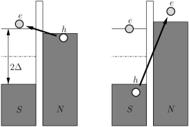
Figure 1: Picture of the virtual electron-hole pairs contributing to the “vacuum correction” of the ground state energy in a superconducting grain near the charge degeneracy point. On the even side of the charge degeneracy points (left panel), without coupling, all electrons in the grain are accommodated in the condensate. In the presence of the coupling, the virtual states consist of a hole created in the lead and an electron in the grain. On the odd side (right panel), one quasiparticle is inevitably present above the gap and the prevailing virtual states consist in creating a hole in the grain and an electron in the lead, with energy cost at least $2\Delta$. In comparison, the virtual states which result from annihilation of a quasiparticle already present in the grain and creating an electron in the lead do not have such energy cost. However, by construction the number of such virtual states is much smaller than the number of states with the energy gap $2\Delta$. Therefore the former do not contribute significantly to the vacuum correction.

The resulting vacuum corrections, $\Delta E_{e}$ and $\Delta E_{o}$, at the even and odd sides of the step, respectively, are different from each other. This can be easily seen in the second-order perturbation theory in $H_{t}$,

$$\Delta E_{o}-\Delta E_{e}=\frac{g}{2\pi^{2}}\int_{0}^{\infty}d\xi\int_{\Delta}^{\infty}d\epsilon\frac{E_{c}\epsilon}{\sqrt{\epsilon^{2}-\Delta^{2}}}$$ (6)

$$\times\left(\frac{1}{E_{-}}+\frac{1}{E_{+}+2E_{c}}-\frac{1}{E_{+}}-\frac{1}{E_{-}+2E_{c}}\right),$$

where $E_{\pm}=\epsilon+\xi\pm\Delta$. The corrected step position, ${\cal N}^{*}$, to the first order in $g$ is defined by equation

$$2E_{c}({\cal N}^{*}-{\cal N}_{0})=\Delta E_{o}-\Delta E_{e}.$$ (7)

In the limit $\Delta\ll E_{c}$, the result of evaluation of Eq. (6) yields

$${\cal N}^{*}={\cal N}_{0}+\frac{g}{4\pi^{2}}\frac{\Delta}{E_{c}}\left[1+\ln\frac{4E_{c}}{\Delta}\right]>{\cal N}_{0}.$$ (8)

At $(E_{c}-\Delta)\ll E_{c}$, the factor $[1+\ln(4E_{c}/\Delta)]$ in Eq. (8) should be replaced by $\sqrt{2}\ln[1/(3-2\sqrt{2})]\simeq 2.49$. Equation (8) should be viewed as the first two terms of the perturbative expansion for the ${\cal N}^{*}(g)$ function.

When the conductance of the contact increases, the odd plateaus become shorter, as it is shown by Eq. (8). At the same time, the plateaus acquire a finite slope which can also be calculated in the second-order perturbation theory in $H_{t}$ and is of the order of $g/\pi^{2}$ at integer values of ${\cal N}$. The slope must be small for the plateaus to be well defined. When $E_{c}-\Delta\ll E_{c}$, odd plateaus are completely suppressed at $g$ exceeding $7.9(1-\Delta/E_{c})$. Depending on the ratio $\Delta/E_{c}$, this condition can be realized while the even plateaus still remain flat.

In the following, we neglect the small correction to the average grain charge $Q$ related to the finite slope of the plateaus, and determine the large (of the order of $1$) variation of $Q$ which gives the shape of the step separating the “even” and “odd” plateaus in the $Q$ vs. $V_{g}$ dependence.

II.2 shape of the step at zero temperature

The shape of the step is described by the dependence of the average grain charge, $Q=e\langle{\hat{N}}\rangle$, on the gate voltage. At zero temperature, it can be foundmodphyslett by differentiating the ground state energy of the system,

$$\langle{\hat{N}}\rangle_{0}={\cal N}-\frac{1}{2E_{c}}\frac{\partial E_{g}}{\partial{\cal N}}.$$ (9)

The shift of the step position evaluated above comes from the grain charge fluctuations with a typical energy of the order of $\Delta$. On the other hand, the shape of the step is determined by the low-energy excitations. The band width for these excitations is controlled by the closeness to the (shifted) charge degeneracy point. This separation of energy scales allows us to derive an effective low-energy Hamiltonian, $H_{0}$, in which the renormalization of the step position is already accounted for. The new Hamiltonian $H_{0}$ acts in a narrow energy band of width $D\ll\Delta$, and is designed to describe the low-energy physics of the system near the charge degeneracy point,

$$2E_{c}|{\cal N}-{\cal N}^{*}|\lesssim D.$$ (10)

The bandwidth is defined with the energy reference in Hamiltonian $H_{0}$ set as the energy of the odd state obtained from Hamiltonian $H+H_{t}$ in second order perturbation theory. That is, energy $E_{c}(2l+1-{\cal N})^{2}+\Delta+\Delta E_{o}$ is subtracted from the initial Hamiltonian. All the states whose number of electrons on the grain differs from $2l$ or $2l+1$ have energy higher than $2E_{c}$. Thus, they are excluded from the low-energy subspace. Moreover, as a consequence of $D\ll\Delta$, the even states cannot accommodate any excitation in the grain (it would cost at least the energy $2\Delta$), while the odd states accommodate exactly one excitation. Starting from Eqs. (1) and (4) and using the Schrieffer-Wolff transformation, we are able to derive the low-energy Hamiltonian, see Section III. Here we present only the relevant for the discussion terms of that Hamiltonian:

$$H_{0} = \epsilon_{0}\left|0\right>\left<0\right|+\sum_{k\sigma}\frac{\zeta^{2}_{k}}{2\Delta}\left|k\sigma\right>\left<k\sigma\right|+\sum_{p\sigma}\xi_{p}c_{p\sigma}^{\dagger}c_{p\sigma}$$ (11)

$$+\sum_{kp\sigma}\left[\tilde{t}_{kp}\left|k\sigma\right>\left<0\right|c_{p\sigma}+\tilde{t}_{kp}^{*}c^{\dagger}_{p\sigma}\left|0\right>\left<k\sigma\right|\right],$$

Here $\epsilon_{0}$ is the energy of the grain in the “even” state $|0\rangle$; it accounts for the renormalization of the step position by virtual electron-hole pairs with energy exceeding $D$. Up to small terms of the order of $g\sqrt{\Delta D}$, this energy is $\epsilon_{0}=2E_{c}({\cal N}-{\cal N}^{*})$, cf. Eq. (8). The energies of allowed states for the Hamiltonian Eq. (11) are within the band of width $\sim 2D$. States $\left|k\sigma\right>$ have an excitation in state $(k\sigma)$ of the grain with energy $\epsilon_{k}-\Delta\approx\zeta^{2}_{k}/(2\Delta)$. The tunnel matrix elements $\tilde{t}_{kp}=u_{k}t_{kp}\approx(1/\sqrt{2})t_{kp}$ account for the coherence factors values at small energies. Note, that the Hamiltonian (11) allows only for zero or one additional electron in the grain.

With the change of energy reference, Eq. (9) defining the average grain charge must be replaced by

$$\langle{\hat{N}}\rangle_{0}=2l+1-\frac{1}{2E_{c}}\frac{\partial E_{0}}{\partial{\cal N}},$$ (12)

where $E_{0}$ is the ground state energy of Hamiltonian (11).

In the zeroth order in $\tilde{t}_{kp}$, the wave function of an even state is a direct product of $|0\rangle$ for the grain and some state $|f\rangle$ of the Fermi sea in the lead; the ground state is $|0\rangle\otimes|f_{0}\rangle$. Tunneling terms in Eq. (11) modify the eigenfunctions. In the lowest order of perturbation theory, the wave function acquires the form

$$\left|\Psi\right>=\left(A\left|0\right>+\sum_{kq\sigma}\beta_{kq\sigma}c_{p\sigma}\left|k\sigma\right>\right)\otimes\left|f\right>.$$ (13)

The second term in parentheses in Eq. (13) describes amplitude of a quasiparticle-hole pair state created due to the tunneling; this amplitude is small within the perturbation theory. In higher orders of the perturbation theory, additional electron-hole pairs may be created in the normal lead. However, as we show in the next Section, these additional terms are small if the number $N_{\rm ch}$ of quantum channels in the junction is large. In the simplest case, the number of channels is of the order of the junction area measured in units of the Fermi wavelength in the metallic electrodes (see Sec. III for details), and the condition $N_{\rm ch}\gg 1$ is not restrictive. If it is satisfied, the wavefunction Eq. (13) is valid beyond the perturbation theory. Having this in mind, for now we may use it as a trial function for an eigenstate originating from the state $|f\rangle$ in the absence of tunneling. Then the ground state energy is the lowest value of $E_{0}$ which solves the equation

$$E=\epsilon_{0}+\sum_{kp\sigma}\frac{\left|\tilde{t}_{kp}\right|^{2}\theta(-\xi_{p})}{E-\zeta^{2}_{k}/(2\Delta)+\xi_{p}}.$$ (14)

This lowest-energy solution

$$E_{0}({\cal N}) = -2E_{c}\delta{\cal N}\left(\sqrt{1+\frac{{\cal N}^{*}-{\cal N}}{\delta{\cal N}}}-1\right)^{2}\theta({\cal N}^{*}-{\cal N}),$$

$$\delta{\cal N} = \left(\frac{g}{8\pi}\right)^{2}\frac{\Delta}{E_{c}},$$ (15)

is separated at ${\cal N}<{\cal N}^{*}$ from the continuum of states $E>0$ allowed by Eq. (14) and can be associated with a bound state. This state is formed by the quasiparticle (virtually) populating the grain and the corresponding hole in the lead. Upon approaching the threshold value ${\cal N}={\cal N}^{*}$, the binding energy of this state vanishes, $E_{0}({\cal N})\propto({\cal N}-{\cal N}^{*})^{2}$. At ${\cal N}\geq{\cal N}^{*}$ the hole is not localized near the junction any more; the formerly discrete energy level merges with the edge of the continuum spectrum. The described qualitative change of the spectrum at the even-odd transition is identical to the one in a well-known problem of single-particle quantum mechanics. Indeed, the same transformation occurs with the spectrum of a particle attracted to a three-dimensional well upon the gradual reduction of the well depth; particle becomes delocalized at a certain strength of the potential,Fano and the discrete energy level ceases to exist.

The number of electrons in the grain at zero temperature is obtained from Eqs. (12) and (15):

$$\langle{\hat{N}}\rangle_{0} = 2l+1-\theta({\cal N}^{*}-{\cal N})f\left(\frac{{\cal N}^{*}-{\cal N}}{\delta{\cal N}}\right)\,,$$

$$f(x) = 1-\frac{1}{\sqrt{1+x}}.$$ (16)

Eq. (16) describes the transition between the “even” plateau with $2l$ electrons in the grain and the “odd” plateau with $2l+1$ electrons. The dependence of $\langle{\hat{N}}\rangle_{0}$ on ${\cal N}$ is shown in Fig. 2.

Figure 2: Coulomb staircase at different temperatures $T=0$ (thick line) and $T=10,20,50T_{q}$. $\langle{\hat{N}}\rangle$ is the average number of electrons in the grain, $V_{g}$ is the gate voltage. The plots correspond to the following values of parameters: $g=2$, $\Delta/E_{c}=0.7$, $\sqrt{8\pi}\Delta/\delta=10^{4}$. With these parameters, $T^{*}\approx 0.1\Delta$, $T_{q}\approx 0.001\Delta$, and ${\cal N}^{*}\approx 2l+0.8$. The correction due to the finite slope of the steps at integer values of $C_{g}V_{g}/e$ is not accounted for in the plots.

At the degeneracy point (${\cal N}={\cal N}^{*}$), the charge is a continuous function of ${\cal N}$, but there is a jump in the differential capacitance, $C_{\text{diff}}=C_{g}d\langle{\hat{N}}\rangle_{0}/d{\cal N}$. We can define the step position by equation $\langle{\hat{N}}\rangle_{0}=2l+\frac{1}{2}$ and characterize the step width by the value of $W_{0}=(d\langle{\hat{N}}\rangle_{0}/d{\cal N})^{-1}$ at the step position. The smearing of the steps of the Coulomb staircase occurs in the second-order in $g$, with a typical width $W_{0}=16\delta{\cal N}$.

II.3 shape of the step at finite temperature

We turn now to the effect of a finite temperature, $T$, on the average grain charge, $\langle{\hat{N}}\rangle$. Equation (12) can still be used, except that $E_{0}$ should be replaced with the free energy $F=-T\ln Z$, where

$$Z=\mathrm{Tr}\exp\left(-\beta H_{0}\right)$$ (17)

is the partition function of the systemmodphyslett described by Hamiltonian (11).

To compute $Z$, we must determine the energies of the excited states. For that we once again will be using Eq. (13) as a trial wave function. The corresponding eigenenergy can be represented in the form $E={\cal E}_{f}+{\cal E}$. Here ${\cal E}_{f}$ is the energy of the “bare” state $|f\rangle$. In the limit of a thermodynamically large lead, ${\cal E}$ is a solution of the already used Eq. (14), where the step function $\theta(\xi)$ should be replaced by the Fermi distribution function. Similarly to the zero temperature case there are two classes of solutions at ${\cal N}<{\cal N}^{*}$. In the first class there is just one discrete solution whose energy at low temperatures is ${\cal E}=E_{0}$, see discussion in the paragraph below Eq. (19). The second class is represented by continuum spectrum ${\cal E}=\zeta_{k}^{2}/(2\Delta)-\xi_{p}$. The full energy for a state in the second class can be written in the form $E={\cal\bar{E}}_{f}+\zeta^{2}/(2\Delta)$, where ${\cal\bar{E}}_{f}$ is the energy of the state that differs from $|f\rangle$ by the presence of one hole in state $p$. Since the partition function involves summation over all states the difference between ${\cal\bar{E}}_{f}$ and ${\cal E}_{f}$ drops out and we have,

$$Z=\sum_{f}e^{-\beta({\cal E}_{f}+E_{0})}+\sum_{f,k\sigma}e^{-\beta({\cal E}_{f}+\zeta^{2}_{k}/(2\Delta))}.$$ (18)

Factorizing the ${\cal N}$-independent partition function of the lead, $Z_{\text{lead}}=\sum_{f}e^{-\beta{\cal E}_{f}}$, and integrating the second term over $k$, we get

$$Z=Z_{\text{lead}}\left[e^{-\beta E_{0}}+N_{\text{eff}}(T)\right],\quad N_{\text{eff}}(T)=\sqrt{\frac{8\pi\Delta T}{\delta^{2}}},$$ (19)

where $\delta$ is the one-electron level spacing in the grain. A rigorous derivation of the finite-temperature partition function is detailed in Section IV.

We would like to note that the replacement of $\theta(\xi)$ by the Fermi function in Eq. (14) leads to a small difference between the energy of the discrete state and $E_{0}$. This finite temperature correction is small in $T/E_{0}$. For the purpose of evaluating the partition function this correction can be ignored at all temperatures because at $T/E_{0}\gtrsim 1/\ln N_{\text{eff}}(T)$, see Eq. (19), the partition function is already dominated by the contribution from the states of the continuum, while $T/E_{0}$ is still small.

Using Eq. (12), we obtain the average grain charge at finite temperature

$$\langle{\hat{N}}\rangle=2l+1-\frac{\theta({\cal N}^{*}-{\cal N})}{1+N_{\text{eff}}(T)e^{\beta E_{0}({\cal N})}}f\left(\frac{{\cal N}^{*}-{\cal N}}{\delta{\cal N}}\right),$$ (20)

where $E_{0}({\cal N})$ and $f(x)$ are defined in Eqs. (15) and (16), respectively.

The temperature dependence of the Coulomb staircase is shown in Fig. 2. At $T\to 0$ Eq. (20) reproduces the average charge, $\langle{\hat{N}}\rangle_{0}$, given by Eq. (16). At finite temperature, the odd plateaus become broader. The position of the step, defined by equation $\langle{\hat{N}}\rangle=2l+\frac{1}{2}$, results from the competition between the energy of the grain in an even state, $E_{0}$, and the entropy of the large number of odd states, given by $N_{\text{eff}}(T)$ in Eq. (19). The step is shifted from ${\cal N}={\cal N}^{*}$ to ${\cal N}={\cal N}^{*}(T)$,

$${\cal N}^{*}(T)={\cal N}^{*}-\frac{T}{2E_{c}}\ln N_{\text{eff}}(T)$$ (21)

when

$$T\gtrsim T_{q}=\left(\frac{g}{8\pi}\right)^{2}\frac{\Delta}{\ln\frac{g\Delta}{\delta\sqrt{8\pi}}},$$ (22)

that is when the shift exceeds the zero-temperature width of the step, $W_{0}=16\delta{\cal N}$. Note that the thermal width $W_{T}=T/E_{c}$ of the charge step at $T\gtrsim T_{q}$ is smaller than that at zero temperature, $W_{T_{q}}\lesssim W_{0}$. We thus expect a strong nonmonotonic temperature dependence of the step width with the minimum width occurring at $T\sim T_{q}$. The temperature dependence of the step position and width are shown in Fig. 3.

Figure 3: Temperature dependence of the step position, ${\cal N}^{*}(T)$, and width $W_{T}$. The same values of parameters as in fig. 2 is used.

The junction conductance $g$ does not affect the charge steps at $T\gg T_{q}$. At even larger temperature, $T\sim T^{*}=\Delta/\ln(\sqrt{8\pi}\Delta/\delta)$, the “odd” plateaus were shown to reach the same size as the “even” ones.modphyslett

In the rest of the paper, we aim at giving a rigorous derivation of the main results, Eqs. (15), (16), and (20) . We’ll show that they hold for the experimentally relevant case of a wide multichannel junction between the grain and the lead. In Section III, we derive the low-energy effective Hamiltonian (11); we demonstrate there that the corrections in the number of channels to the ground state energy, are small. In Section IV, we derive the partition function for our system.

III Effective Hamiltonian and the grain charge at zero temperature

In this Section we derive the effective low-energy Hamiltonian (11) which is used to describe the shape of the step of the Coulomb staircase between the even state of the grain with a charge $Q=(2l)e$ and the odd state with a charge $Q=(2l+1)e$. We show that it gives the same physics as the Hamiltonian of the system, $H+H_{t}$, given by Eqs. (1) and (4), for a wide multichannel contact between the grain and the lead.

The effective Hamiltonian $H_{0}$ is acting in a narrow bandwidth $D$, on a limited set of states which was characterized in Section II: only low-energy electrons (or holes) may be excited in the lead, and the states of the grain are only those with zero or one low-energy excitation,

$$|\xi_{k}|,E_{c}({\cal N}^{*}-{\cal N})+\zeta^{2}/2\Delta\lesssim D.$$

The states outside the bandwidth $D$ are accounted in $H_{0}$ perturbatively. For the present problem, it is enough to calculate such contribution in the second order in $H_{t}$. Therefore, the appropriate Schrieffer-Wolff transformation of the initial Hamiltonian is QM

$$H_{0}\approx M(H+H_{t})M-MH_{t}(1-M)\frac{1}{H}H_{t}M.$$ (23)

Here, $M$ is the projector operator on the unperturbed states whose energy lies within the band $D$. We obtain

$$H_{0} =H^{\prime}+V,$$ (24)

$$H^{\prime} =\epsilon_{0}P_{e}+\sum_{k\sigma}\frac{\zeta^{2}_{k}}{2\Delta}P_{o}\gamma^{\dagger}_{k\sigma}\gamma_{k\sigma}P_{o}+\sum_{p\sigma}\xi_{p}c^{\dagger}_{p\sigma}c_{p\sigma}$$

$$V =\sum_{kp\sigma}\left[\tilde{t}_{kp}P_{o}\gamma^{\dagger}_{k\sigma}c_{p\sigma}P_{e}+\tilde{t}_{kp}^{*}P_{e}c^{\dagger}_{p\sigma}\gamma_{k\sigma}P_{o}\right]$$

$$+\sum_{p\neq p^{\prime}\sigma}\sum_{i=e,o}w_{pp^{\prime}}^{i}c_{p\sigma}^{\dagger}c_{p^{\prime}\sigma}P_{i}+\sum_{k\neq k^{\prime}\sigma}w_{kk^{\prime}}P_{o}\gamma^{\dagger}_{k\sigma}\gamma_{k^{\prime}\sigma}P_{o}.$$

Here, $P_{e}$ and $P_{o}$ are projection operators on the even and odd states with $2l$ or $2l+1$ electrons in the grain, respectively, $\tilde{t}_{kp}=u_{k}t_{kp}$, and

$$\epsilon_{0}=2E_{c}({\cal N}_{0}-{\cal N}^{*})+\sum_{kp\sigma}^{\prime}\frac{\left|\tilde{t}_{kp}\right|^{2}\theta(-\xi_{p})}{\frac{\zeta^{2}_{k}}{2\Delta}-\xi_{p}}.$$ (25)

The prime here means that only excited states in the bandwidth $D$, (i.e., such as $|\zeta^{2}_{k}/(2\Delta)-\xi_{p}|<D$) are included. Making the summation on $k$ and $p$, we obtain

$$\epsilon_{0}\approx 2E_{c}\left({\cal N}-{\cal N}^{*}+\frac{g}{2\pi^{2}}\frac{\sqrt{2\Delta D}}{2E_{c}}\right).$$ (26)

The degeneracy point ${\cal N}$ defined by condition $\epsilon_{0}=0$ would slightly differ from ${\cal N}^{*}$. This difference comes from the virtual states with energies within the band $D$; such states were accounted for in the evaluation of ${\cal N}^{*}$, but do not contribute to $\epsilon_{0}$. This difference is small at small ($D\ll\Delta$) bandwidth. Note, that by construction of the Hamiltonian $H_{0}$, we need energy $\epsilon_{0}$ at ${\cal N}={\cal N}^{*}$ to be within the band $D$. This sets a condition $D\gtrsim\frac{g^{2}}{2\pi^{4}}\Delta$, which does not contradict our initial assumption $D\ll\Delta$.

Perturbation $V$ in Eq. (24) has terms describing electron-hole pair fluctuations across the junction, and terms describing scattering off the junction within the grain or lead. The latter terms correspond to second-order processes in $H_{t}$ generated by the Schrieffer-Wolf transformation (23). For instance, the term corresponding to scattering off the lead when the grain is in the even state has probability amplitude

$$w_{pp^{\prime}}^{e}=-\sum^{\prime\prime}_{k}t_{kp^{\prime}}t_{kp}^{*}\left(\frac{u_{k}^{2}}{\epsilon_{k}-\Delta}-\frac{v_{k}^{2}}{2E_{c}+\epsilon_{k}+\Delta}\right).$$ (27)

Here, the first and second term in parentheses correspond to virtual excitations with charge $(2l+1)e$ and $(2l-1)e$ in the grain, respectively; the double-prime means that only virtual states with excitation energy outside the bandwidth are included in the sum, it reduces to condition $\epsilon_{k}-\Delta>D$ for the first term (we also used property $t_{kp}^{*}=t_{-k-p}$ valid for tunneling Hamiltonian preserving the time-reversal symmetry). The amplitudes $w^{o}_{pp^{\prime}}$ and $w_{kk^{\prime}}$ have expressions similar to Eq. (27). We will put terms proportional to $w^{i}_{pp^{\prime}}$ and $w_{kk^{\prime}}$ in $V$ aside for a while and return to the discussion of their effect at the end of the Section.

Let us calculate the ground state energy of $H_{0}$. At ${\cal N}<{\cal N}^{*}$, the unperturbed ground state on the “even” side, $\left|e\right>=|0\rangle\otimes|f_{0}\rangle$, is the direct product of the BCS ground state with $2l$ electrons in the grain, $|0\rangle$, times Fermi sea ground state in the lead, $|f_{0}\rangle$. Its bare energy is $\epsilon_{0}$. In the presence of $V$, we determine its renormalized energy, $E_{0}$, with Brillouin-Wigner perturbation theory.QM It is the solution of the infinite order equation

$$E_{0}=\epsilon_{0}+\left<e\right|V\left|e\right>+\sum_{n\neq 0}\frac{\left<e\right|V\left|n\right>\left<n\right|V\left|e\right>}{E_{0}-\epsilon_{n}}$$ (28)

$$+\sum_{n_{1},\cdots,n_{j}\neq 0}\frac{\left<e\right|V\left|n_{1}\right>\left<n_{1}\right|V\left|n_{2}\right>\cdots\left<n_{j}\right|V\left|e\right>}{(E_{0}-\epsilon_{n_{1}})\cdots(E_{0}-\epsilon_{n_{j}})}+\cdots,$$

where $\left|n\right>$ are eigenstates of $H^{\prime}$, with energy $\epsilon_{n}$. Anticipating that, for typical S-I-N systems with multichannel contacts, the series in the Eq. (28) can be truncated at the term of the second order in $V$, we obtain:

$$E_{0}=\epsilon_{0}+\sum_{kp\sigma}^{\prime}\frac{\left|\tilde{t}_{kp}\right|^{2}\theta(-\xi_{p})}{E_{0}-\frac{\zeta^{2}_{k}}{2\Delta}+\xi_{p}}.$$ (29)

Here again, the prime means that only excited states in the bandwidth $D$ are included. This equation is identical to Eq. (14). As a result of the summation in Eq. (29), the bandwidth $D$ disappears from the equation for the ground state energy and we arrive at Eq. (15).

The above result holds when higher order in $V$ terms can be neglected in Eq. (29). This is the case for a generic tunnel junction between a lead and metallic grain. Indeed, typically the area of junction $S$ exceeds significantly the square of the Fermi wavelength in a metal. The effective number of quantum channels in the junction, $N_{\text{ch}}\sim Sk_{F}^{2}\gg 1$ provides us with a parameter allowing the truncation of series Eq. (29) in the ballistic regime. In a realistic setup, electrons are backscattered to the junction from the impurities and the boundaries in the grain and in the lead. In a typical situation of a small junction to a macroscopic lead the the backscattering of electrons from the lead to the junction may be neglected. We therefore concentrate on the effects of electron returns from the grain to the junction. Due to the finite grain size such returns are bound to occur. Quantum interference between returning electron trajectories in the grain may lead to a reduction of $N_{\text{ch}}$.Hekking However, we shall see that the corresponding contribution to Eq. (16) remains small in the parameter $1/N_{\rm ch}^{\rm eff}=\delta/g\Delta\ll 1$.

We start with the analysis of higher-order perturbation theory terms which involve matrix elements ${\tilde{t}}_{kp}$ only. Let us first consider the “even” side of the transition, at ${\cal N}<{\cal N}^{*}$. The first term in Eq. (28) that we neglect is

$$J=\sum_{kk^{\prime}pp^{\prime}\sigma}^{\prime}\frac{\theta(-\xi_{p})\theta(\xi_{p^{\prime}})\tilde{t}_{kp}\tilde{t}_{kp^{\prime}}^{*}\tilde{t}_{k^{\prime}p^{\prime}}\tilde{t}_{k^{\prime}p}^{*}}{[E_{0}-\epsilon_{kp}][E_{0}-\epsilon_{pp^{\prime}}][E_{0}-\epsilon_{k^{\prime}p}]},$$ (30)

where $\epsilon_{kp}=\zeta^{2}_{k}/(2\Delta)-\xi_{p}$ and $\epsilon_{p^{\prime}p}=\epsilon_{0}+\xi_{p^{\prime}}-\xi_{p}$, and the prime means that $|\epsilon_{kp}|,|\epsilon_{k^{\prime}p}|,|\epsilon_{p^{\prime}p}|<D$. We define the correlation function

$$K(\xi,\xi^{\prime};\zeta,\zeta^{\prime})=\sum_{kk^{\prime}pp^{\prime}}t_{kp}t_{kp^{\prime}}^{*}t_{k^{\prime}p^{\prime}}t_{k^{\prime}p}^{*}\delta(\xi-\xi_{p})$$

$$\times\delta(\xi^{\prime}-\xi_{p^{\prime}})\delta(\zeta-\zeta_{k})\delta(\zeta^{\prime}-\zeta_{k^{\prime}}),$$ (31)

which simplifies Eq. (30) to

$$J=-\int^{\prime}d\xi d\xi^{\prime}d\zeta d\zeta^{\prime}\frac{\theta(-\xi)\theta(\xi^{\prime})K(\xi,\xi^{\prime};\zeta,\zeta^{\prime})}{[\epsilon_{\zeta\xi}-E_{0}][\epsilon_{\xi^{\prime}\xi}-E_{0}][\epsilon_{\zeta^{\prime}\xi}-E_{0}]},$$ (32)

with $\epsilon_{\zeta\xi}=\zeta^{2}/(2\Delta)-\xi$ and $\epsilon_{\xi^{\prime}\xi}=\epsilon_{0}+\xi^{\prime}-\xi$; the prime means $|\epsilon_{\zeta\xi}|,|\epsilon_{\xi^{\prime}\xi}|,|\epsilon_{\zeta^{\prime}\xi}|<D$.

The value of $J$ depends on a concrete model of the junction. We consider here a thin homogeneous insulating layer separating the grain from lead; the appropriate barrier potential is $U(\mathbf{r})=U_{0}\delta(z)$, where $z$ is the distance from the interface. The transmission coefficient ${\cal T}$ for such a barrier depends on the angle of incidence for the incoming electron characterized by the normal component $k_{z}$ of its momentum $\mathbf{k}$; in the limit of low barrier transparency ${\cal T}(k_{z})=(k_{z}/mU_{0})^{2}\ll 1$. The dimensionless conductance of the junction is $g={\cal T}Sk_{F}^{2}/4\pi$, where $k_{F}$ is the Fermi wavevector and $S$ is the area of the junction and ${\cal T}={\cal T}(k_{F})$. We can introduce the number of channels in the junction by expressing the conductance $g={\overline{\cal T}}N_{\rm ch}$ in terms of the angle-averaged transmission coefficient, ${\overline{\cal T}}={\cal T}/3$. This definition of $N_{\rm ch}$ yields $N_{\rm ch}=3Sk_{F}^{2}/4\pi$. In terms of the matrix elements in the tunneling Hamiltonian, the above model of the barrier corresponds to

$$t_{\mathbf{kp}}=\frac{\sqrt{\cal T}}{\nu\sqrt{V_{l}V}}k_{z}p_{z}\delta^{2}(\mathbf{k}_{\|}-\mathbf{p}_{\|}).$$ (33)

with $\nu=(mk_{F}/2\pi^{2})$, $V$, and $V_{l}$ being the density of states, volume of the grain and volume of the lead, respectively; $m$ is the effective electron mass. Equation (33) accounts for the conservation of the component $\mathbf{k}_{\|}$ of the electron momentum parallel to the barrier. Inserting now Eq. (33) into (31), we obtain the correlation function in the ballistic regime

$$K_{\text{b}}(\xi,\xi^{\prime};\zeta,\zeta^{\prime})=\frac{3g^{2}}{8\pi^{4}N_{\text{ch}}}.$$ (34)

We can now evaluate Eq. (32). It yields the dominant contribution in $|E_{0}|$:

$$J_{\text{b}}=-\frac{g^{2}}{8\pi^{2}N_{\text{ch}}}\Delta\ln\frac{D}{-E_{0}}\ln\frac{D}{\epsilon_{0}}.$$ (35)

In the vicinity of the degeneracy point, at ${\cal N}^{*}-{\cal N}\lesssim\delta{\cal N}$, the energy $E_{0}$ is much smaller than $\epsilon_{0}\propto g(\Delta D)^{1/2}$, as the bandwidth $D$ satisfies the conditions $\frac{g^{2}}{2\pi^{2}}\Delta\ll D\ll\Delta$. Therefore, the logarithmic term $\ln(D/\epsilon_{0})$ in Eq. (35) is approximately constant and of the order of $\ln(1/g)$. As the result, for a grain in the “ballistic” regime, the contribution (35) yields a correction to the grain charge

$$\delta Q\sim e\frac{\ln(1/g)}{N_{\rm ch}}\frac{\delta{\cal N}}{{\cal N}^{*}-{\cal N}}$$ (36)

which is small outside the region ${\cal N}^{*}-{\cal N}\sim\delta{\cal N}/N_{\text{ch}}$; this region is much smaller than $\delta{\cal N}$.

The ballistic estimate Eq. (35) holds if the virtual excitation in the grain travels a distance shorter than the grain size $L$ and the electron mean free path $\ell$; for definiteness, we assume $L\lesssim\ell$. The length of the path of the excitation depends on its typical energy given by $|E_{0}|$. Indeed, the velocity of excitation is $v\sim v_{F}\zeta/\Delta$, and the time of travel is limited by $1/|E_{0}|$; here $v_{F}$ is the Fermi velocity. The limitation on the excitation path length sets the condition for the applicability of the ballistic approximation, $\Delta|E_{0}|\gtrsim v_{F}^{2}/L^{2}$. The condition is violated sufficiently close to the charge degeneracy point,

$${\cal N}^{*}-{\cal N}\sim\frac{gv_{F}}{E_{c}L}.$$ (37)

Here we assumed sufficiently large $N_{\rm ch}$, so that the interval of ${\cal N}$ defined by Eq. (37) is shorter than $\delta{\cal N}$. We turn now to the estimate of the fourth-order term (30) deep inside this interval.

If an excitation bounces off the grain walls many times, it is reasonable to expect chaotization of its motion. This prompts one to consider ensemble-averaged observables, rather than their specific values for a given grain. To this end, we need to express $J$ of Eq. (30) in terms of the correlation functions of the electron states in the grain. We start with representing prada the matrix elements $t_{kp}$ in terms of the true electron eigenstates $\phi^{*}_{k}$ and $\chi_{p}$,

$$t_{kp}=\frac{\sqrt{\cal T}}{8\pi^{2}\nu}\int_{S}d^{2}\mathbf{x}\left.\partial_{z}\phi^{*}_{k}(\mathbf{r})\partial_{z}\chi_{p}(\mathbf{r})\right|_{z=0}.$$ (38)

Here, $\mathbf{x}$ is the longitudinal with respect to the barrier component of coordinate $\mathbf{r}$. Inserting Eq. (38) into (5) and averaging independently the states in the grain and in the lead, we can express the conductance

$$g=\frac{{\cal T}}{8\pi^{2}\nu^{2}}\int_{S}d^{2}\mathbf{x}d^{2}\mathbf{x}^{\prime}\partial_{z}\partial_{z^{\prime}}K_{\zeta\approx 0}(\mathbf{r},\mathbf{r}^{\prime})$$

$$\times\left.\partial_{z}\partial_{z^{\prime}}K_{\xi\approx 0}(\mathbf{r}^{\prime},\mathbf{r})\right|_{z=z^{\prime}=0},$$ (39)

in terms of the ensemble-averaged Green’s function in the grain,

$$K_{\zeta}(\mathbf{r},\mathbf{r}^{\prime})\equiv-\frac{1}{\pi}\mathrm{Im}G^{R}_{\zeta}(\mathbf{r},\mathbf{r}^{\prime})=\overline{\sum_{k}\phi_{k}(\mathbf{r})\phi^{*}_{k}(\mathbf{r}^{\prime})\delta(\zeta-\zeta_{k})},$$ (40)

and similarly in the lead $K_{\xi}\equiv(-1/\pi)\mathrm{Im}G^{R}_{\xi}$. As the conductance is determined by tunneling events taking place on the spatial range $1/k_{F}$ close to the junction, it is enough to take the Green’s functions for half-infinite spaces with the appropriate boundary condition that they vanish at the interface. Averaging each of them independently on the disorder in the metals, we recover the result $g={\overline{\cal T}}N_{\text{ch}}$ of the ballistic regime. At the same time, the correlation function (31) is strongly affected by the disorder.Hekking Expressing Eq. (31) in terms of the Green’s functions in the metals and ensemble-averaging the product of two Green’s functions, the authors of Ref. Hekking, obtained

$$K_{\text{d}}(\xi,\xi^{\prime};\zeta,\zeta^{\prime})=\frac{g^{2}}{128\pi^{5}\nu}\int\frac{d^{2}\mathbf{x}d^{2}\mathbf{x}^{\prime}}{S^{2}}\left[P_{\zeta^{\prime}-\zeta}(\mathbf{r}^{\prime},\mathbf{r})\right.$$

$$\left.+P_{\zeta-\zeta^{\prime}}(\mathbf{r},\mathbf{r}^{\prime})\right]_{z=z^{\prime}=0}.$$ (41)

Here $P_{\omega}(\mathbf{r},\mathbf{r}^{\prime})$ describes the evolution of the probability density to find an electron at a given point $\mathbf{r}$. For diffusive motion (under the condition $\ell\ll L$), the diffuson $P_{\omega}(\mathbf{r},\mathbf{r}^{\prime})$ obeys the diffusion equation,

$$\left(i\omega-D\mathbf{\nabla}_{\mathbf{r}}^{2}\right)P_{\omega}(\mathbf{r},\mathbf{r}^{\prime})=\delta^{3}(\mathbf{r}-\mathbf{r}^{\prime}),$$ (42)

and $D=(v_{F}\ell)/3$ is the diffusion constant in the grain. At frequencies $\omega$ smaller than the Thouless energy $D/L^{2}$, the solution of Eq. (42) reaches the universal (zero-mode) limit where

$$P_{\omega}(\mathbf{r},\mathbf{r}^{\prime})+P_{-\omega}(\mathbf{r}^{\prime},\mathbf{r})\approx\frac{2\pi}{V}\delta(\omega)$$ (43)

is independent of the coordinates in the grain. In the case of a smaller grain, $L\lesssim\ell$, Eq. (42) does not hold, but the universal limit for $P_{\omega}(\mathbf{r},\mathbf{r}^{\prime})$ is the same ABG , and is reached at $\omega\lesssim v_{F}/L$. With the help of Eq. (43), we may now evaluate Eq. (32) to find

$$J_{\text{d}}\approx-\frac{g^{2}\ln(1/g)}{64\pi^{3}}\,\delta\,\sqrt{\frac{2\Delta}{-E_{0}}}.$$ (44)

Here $\delta=1/\nu V$ is the electron level spacing in the grain. Equation (44) yields (in the region ${\cal N}^{*}-{\cal N}\ll\delta{\cal N}$) a correction to the charge of the order

$$\delta Q\sim e\frac{\ln(1/g)}{N_{\rm ch}^{\rm eff}}\left(\frac{\delta{\cal N}}{{\cal N}^{*}-{\cal N}}\right)^{2},\quad\frac{1}{N_{\rm ch}^{\rm eff}}=\frac{\delta}{g\Delta}$$ (45)

Comparing Eqs. (36) and (45), we see that they match each other at the gate voltage given by Eq. (37). The latter defines the crossover between the ballistic and “zero-mode” limits, and corresponds to the path length of the virtual excitations of the order of $L$. The correction Eq. (45) remains small everywhere except a very narrow region around the charge degeneracy point, ${\cal N}^{*}-{\cal N}\lesssim\delta{\cal N}/(N_{\rm ch}^{\rm eff})^{1/2}$.

On the odd side of the charge degeneracy point, at ${\cal N}>{\cal N}^{*}$, the unperturbed ground state is $P_{o}\gamma^{\dagger}_{k\sigma}\left|e\right>$, where $k$ is the closest to the Fermi level state. In the zeroth in $1/N_{\rm ch}^{\rm eff}$ limit, the ground state energy is zero. The correction induced in $E_{0}$ by the perturbation $V$ in the Hamiltonian $H_{0}$ is found from equation

$$E_{0}=\sum_{p}^{\prime}\frac{\left|\tilde{t}_{kp}\right|^{2}\theta(\xi_{p})}{E_{0}-\epsilon_{0}-\xi_{p}}.$$ (46)

As the tunneling matrix element involves a single state $k$, its solution should exhibit strong mesoscopic fluctuations. The typical value, however, is easy to find,

$$E_{0}\sim-\frac{1}{2\pi^{2}}g\delta\ln(1/g).$$ (47)

Therefore the coupling to the lead induces a small shift of ${\cal N}^{*}$ which scales proportionally to the one-level spacing in the grain and is of the order of $g\delta/E_{c}$. Beyond this small shift, the ground state energy at ${\cal N}>{\cal N}^{*}$ is not modified by perturbation $V$.

Now we return briefly to the effect of the terms proportional to $w_{kk^{\prime}}$ and $w_{pp^{\prime}}^{i}$ in $V$. Indeed, they do also contribute to the Brillouin-Wigner expansion (28) and give correction to the ground state energy (15). In particular, at ${\cal N}<{\cal N}^{*}$, the fourth-order-in-$H_{t}$ corrections to $E_{0}$ formed with such terms are given by integrals similar to Eq. (32). They only differ by the energy ranges of integration which account for the virtual states outside the bandwidth involved in the evaluation of $w_{kk^{\prime}}$ and $w_{pp^{\prime}}^{i}$. The resulting correction is of the same order as, and not more singular at ${\cal N}\to{\cal N}^{*}$ than the contributions we have already evaluated, see Eqs. (35) and (44).

To summarize this Section, we have demonstrated that in the case of a wide junction ($N_{\rm ch}\gg 1$) corrections to the ground state energy Eq. (15) are parametrically small. The smearing of the non-analytical ${\cal N}$–dependence of the grain charge, see Eq. (16) vanishes in the limit of zero level spacing $\delta$ in the grain. Identifying $\left|0\right>$ and $\left|k\sigma\right>$ with $P_{e}\left|\Phi\right>$ and $P_{o}\gamma^{\dagger}_{k\sigma}\left|\Phi\right>$, respectively, where $\left|\Phi\right>$ is the BCS ground state in the grain in the grand-canonical ensemble, and discarding the terms proportional to $w_{kk^{\prime}}$ and $w_{pp^{\prime}}^{i}$ in $V$, we can put Hamiltonian (24) in the form (11).

We note finally that in the opposite limit of a point contact, $N_{\rm ch}=1$, instead of the jump in $C_{\rm diff}$ we would find a smooth crossover Pesin of width $\delta{\cal N}$ in the region of even-odd transition.

IV Charge steps at finite temperature

In this Section, starting from the effective Hamiltonian (11) for a wide, multichannel contact between the superconducting grain and a normal lead, we derive rigorously Eq. (19) which gives the partition function of the system near the charge degeneracy point ${\cal N}^{*}$.

IV.1 Density of states

To compute $Z$, we must determine the excited states.

Without coupling, the many-body “even” eigenstates of the system without excitation in the grain are denoted $|0,f\rangle\equiv|0\rangle\otimes|f\rangle$. We recall that $|0\rangle$ is the wavefunction for the grain in the even state, while $|f\rangle$ is the wavefunction of the lead corresponding to a particular set $f\equiv\{n_{p\sigma}\}$ of electron occupation numbers for each state $(p\sigma)$. The energy of the state $|0,f\rangle$ is ${\cal E}_{f}+\epsilon_{0}$, where

$${\cal E}_{f}=\sum_{p\sigma}\xi_{p}\left(n_{p\sigma}-\theta(\xi_{p})\right)$$ (48)

is the excitation energy for the lead in state $|f\rangle$. The many-body “odd” states with one excitation in state $(k\sigma)$ in the grain are $|k\sigma,f\rangle\equiv|k\sigma\rangle\otimes|f\rangle$, their energy is ${\cal E}_{f}+\zeta^{2}_{k}/(2\Delta)$.

At finite coupling, even and odd state hybridize. In order to find the eigenergies, we can still use Brillouin-Wigner perturbation theory like we did for determining the ground state energy in Section III. Starting from an unperturbed eigenstate $|0,f\rangle$, we can write the Brillouin-Wigner equation for its energy in the presence of the coupling by replacing $\{|e\rangle,\epsilon_{0},E_{0}\}$ with $\{|0,f\rangle,{\cal E}_{f}+\epsilon_{0},E\}$ in Eq. (28). The solutions of this equation are the exact eigenenergies. For a wide junction (in the limits $\delta\to 0$ and $N_{\text{ch}}\to\infty$), such equation can still be truncated up to second order terms in the perturbation $V$, like in Section III. However the Brillouin-Wigner equation generalizing Eq. (29)

$$E=\epsilon_{0}+{\cal E}_{f}+\sum_{kq\sigma}^{\prime}\frac{\left|\tilde{t}_{kq}\right|^{2}n_{q\sigma}}{E-{\cal E}_{f}+\xi_{q}-\zeta^{2}_{k}/(2\Delta)},$$ (49)

now defines a large number of excited states and is impractical to solve for each of them. The prime in the sum means that only unperturbed eigenstates in the bandwidth $D$ are included in the sum. Here, let us note that Eq. (29) is obtained from (49) for the particular set $f_{0}=\{n_{p\sigma}\}$ determined by the Fermi function at zero temperature, $n_{p\sigma}=\theta(-\xi_{p})$, and with the property ${\cal E}_{f_{0}}=0$ . At zero temperature, we were only looking for the solution with lower energy, corresponding to the ground state.

The partition function (17) which is the sum over the full set of eigenstates $E_{\lambda}$ can be expressed in terms the exact density of states, $\nu(E)$:

$$Z=\int_{-\infty}^{\infty}dE\nu(E)e^{-\beta E},$$ (50)

where $\nu(E)=\sum_{\lambda}\delta(E-E_{\lambda})$. The density of state is related to the exact Green’s function $G_{E}=(E-H_{0})^{-1}$ at energy $E$:

$$\nu(E)=-\frac{1}{\pi}\mathrm{Im}\,\mathrm{Tr}\,G_{E_{+}},\quad E_{+}=E+i0^{+}.$$ (51)

We evaluate $\mathrm{Tr}\,G$ in the basis of the unperturbed eigenstates $|0,f\rangle$ and $|k\sigma,f\rangle$. Thus we can write the density of states

$$\nu(E)=-\frac{1}{\pi}\mathrm{Im}\left[\sum_{f}G_{E_{+}}(0,f)+\sum_{k\sigma,f}G_{E_{+}}(k\sigma,f)\right]$$ (52)

in terms of the diagonal elements of $G_{E}$ in this basis:

$$G_{E}(0,f) = \langle 0,f|(E-H_{0})^{-1}|0,f\rangle,$$ (53a)

$$G_{E}(k\sigma,f) = \langle k\sigma,f|(E-H_{0})^{-1}|k\sigma,f\rangle.$$ (53b)

In order to evaluate $G_{E}(0,f)$, we need to introduce the additional matrix elements of $G_{E}$

$$G_{E}(0,f;0,f^{\prime}) = \langle 0,f|(E-H_{0})^{-1}|0,f^{\prime}\rangle,$$ (54a)

$$G_{E}(k\sigma,f;0,f^{\prime}) = \langle k\sigma,f|(E-H_{0})^{-1}|0,f^{\prime}\rangle.$$ (54b)

They solve the closed set of equations

$$\delta_{ff^{\prime}} = (E-{\cal E}_{f}-\epsilon_{0})G_{E}(0,f;0,f^{\prime})$$ (55a)

$$-\sum_{kq\sigma}^{\prime}\tilde{t}_{kq}n_{q\sigma}G_{E}(k\sigma,f_{q\sigma};0,f^{\prime}),$$

$$0 = (E-{\cal E}_{f}-\zeta^{2}_{k}/(2\Delta))G_{E}(k\sigma,f;0,f^{\prime})$$ (55b)

$$-\sum_{q}^{\prime}\tilde{t}_{kq}^{*}(1-n_{q\sigma})G_{E}(0,f^{q\sigma};0,f^{\prime}),$$

Here we defined $\delta_{ff^{\prime}}=1$ if all the electron occupation numbers in the sets $f$ and $f^{\prime}$ coincides, otherwise $\delta_{ff^{\prime}}=0$. Moreover, the set $f_{q\sigma}$ (respectively $f^{q\sigma}$) coincides with $f$, except for the occupation number in state $(q\sigma)$ which is set to $n_{q\sigma}=0$ (respectively $n_{q\sigma}=1$). Inserting (55b) into (55a), and defining the self-energy

$$\widetilde{\Sigma}_{E}(0,f)=\sum_{kq\sigma}^{\prime}\frac{|\tilde{t}_{kq}|^{2}n_{q\sigma}}{E-{\cal E}_{f}+\xi_{q}-\zeta^{2}_{k}/(2\Delta)}$$ (56)

we get the equation

$$\delta_{ff^{\prime}}=(E-{\cal E}_{f}-\epsilon_{0}-\widetilde{\Sigma}_{E}(0,f))G_{E}(0,f;0,f^{\prime})$$ (57)

$$-\sum_{k,p\neq q,\sigma}^{\prime}\frac{\tilde{t}_{kq}\tilde{t}^{*}_{kp}n_{q\sigma}(1-n_{p\sigma})}{E-{\cal E}_{f}+\xi_{q}-\zeta^{2}_{k}/(2\Delta)}G_{E}(0,[f_{q\sigma}]^{p\sigma};0,f^{\prime})$$

The second term in the r.h.s of this equation gives a negligible contribution in the limit $N_{\text{ch}}\to\infty$. (This can be shown along the same lines as in Section III.) As a result, we find

$$G_{E}(0,f)\equiv G_{E}(0,f;0,f)=[E-{\cal E}_{f}-\epsilon_{0}-\widetilde{\Sigma}_{E}(0,f)]^{-1}.$$ (58)

The last term in Eq. (25) defining $\epsilon_{0}$ depends on bandwidth $D$. By subtracting this term from $\epsilon_{0}$ and adding it to $\widetilde{\Sigma}_{E}(0,S)$, we write the Green’s function (58) equivalently

$$G_{E}(0,f)=[E-{\cal E}_{f}-\omega_{0}-\Sigma_{E}(0,f)]^{-1},$$ (59)

where $\omega_{0}=2E_{c}({\cal N}-{\cal N}^{*})$, and

$$\Sigma_{E}(0,f)=\widetilde{\Sigma}_{E}(0,f)+\epsilon_{0}-\omega_{0}.$$ (60)

Inserting Eqs. (25) and (56) into (60) we obtain

$$\Sigma_{E}(0,f)=\sum_{kq\sigma} \left\{\frac{\left|\tilde{t}_{kq}\right|^{2}n_{q\sigma}}{E-{\cal E}_{f}+\xi_{q}-\zeta^{2}_{k}/(2\Delta)}\right.$$ (61)

$$\left.-\frac{\left|\tilde{t}_{kq}\right|^{2}\theta(-\xi_{q})}{\xi_{q}-\zeta^{2}_{k}/(2\Delta)}\right\}.$$

At high energies $|\xi_{p}|$, the electron occupation numbers asymptotically behave as the zero temperature Fermi function. Therefore, the sum in Eq. (61) is convergent and we don’t need to specify anymore that only the states in the low energy subspace are included in it.

We can determine $G_{E}(k\sigma,f)$ in a similar way. In the same limit $N_{\text{ch}}\to\infty$, we obtain

$$G_{E}(k\sigma,f) = g_{E}(k\sigma,f)+g_{E}(k\sigma,f)^{2}$$ (62)

$$\times\sum_{p}|\tilde{t}_{kp}|^{2}(1-n_{p\sigma})G_{E}(0;f^{p\sigma}).$$

The first term in the r.h.s. of Eq.(62) coincides with the Green’s function for the unperturbed state $|k\sigma,f\rangle$ with one excitation in the grain, $g_{E}(k\sigma,f)=[E-{\cal E}_{f}-\zeta^{2}_{k}/(2\Delta)]^{-1}$. The second term comes from its hybridization with the many-body states with no excitation in the grain.

Inserting Eqs. (59) and (62) into (52), we express the density of states as the sum of different contributions:

$$\nu(E) = \sum_{f}\left[\sum_{k\sigma}\delta(E-{\cal E}_{f}-\frac{\zeta^{2}_{k}}{2\Delta})+\delta\nu_{f}(E)\right],$$ (63)

$$\delta\nu_{f}(E) = -\frac{1}{\pi}\mathrm{Im}\left[G_{E_{+}}(0,f)\left(1-\frac{d\Sigma_{E_{+}}(0,f)}{dE}\right)\right].$$ (64)

In Eq. (63), the sum of $\delta$-functions comes from the first term in Eq. (62) while the terms $\delta\nu_{f}(E)$ come from Eq. (59) and the second term in Eq. (62).

In the next Section, we use Eqs. (63) and (64) to evaluate the partition function. We show that the contribution of $\delta\nu_{f}(E)$, Eq. (64), to the partition function can be approximated by that of a single state with energy $E=E_{0}+{\cal E}_{f}$ and derive Eq. (19) for the partition function. Finally, we show that Eqs. (19) and (20) accurately account for the thermodynamic quantities of the grain in the entire temperature range $T<T^{*}$, and at any sign of ${\cal N}-{\cal N}^{*}$ as well.

IV.2 Partition function

Inserting Eq. (63) into (50), we obtain the partition function

$$Z = \sum_{f}e^{-\beta{\cal E}_{f}}\left(\sum_{k\sigma}e^{-(\beta\zeta^{2}_{k}/2\Delta)}\right.$$ (65)

$$+\left.\int^{\infty}_{-\infty}d\omega e^{-\beta\omega}\delta\nu_{f}(\omega+{\cal E}_{f})\right).$$

Introducing the reduced partition function of the grain, $\widetilde{Z}=Z/Z_{\text{lead}}$ and inserting Eqs. (59) and (60) into (64) we obtain

$$\widetilde{Z}=N_{\text{eff}}(T)-\int^{\infty}_{-\infty}d\omega\frac{e^{-\beta\omega}}{\pi}\mathrm{Im}\left\langle\frac{1-d\Sigma_{f}(\omega_{+})/d\omega}{\omega_{+}-\omega_{0}-\Sigma_{f}(\omega_{+})}\right\rangle_{T}.$$ (66)

$Z_{\text{lead}}$ and $N_{\text{eff}}(T)$ were defined in Eq. (19). In the second term of Eq. (66), $\langle\ldots\rangle_{T}$ denotes thermal averaging over with the Hamiltonian of the isolated lead and we introduced the reduced self-energy

$$\Sigma_{f}(\omega)=\Sigma_{\omega+{\cal E}_{f}}(0,f).$$ (67)

The integrand in the second term in Eq. (66) is a regular function of the occupation numbers $n_{p\sigma}$. We can expand the integrand in series in the set of $n_{p\sigma}$. Then we replace them by their thermal average $f(\xi_{p})=[1+\exp(\beta\xi_{p})]^{-1}$ (Their fluctuations $\langle[n_{p\sigma}-f(\xi_{p})]^{2}\rangle_{T}$ scale as the inverse number of electrons in the lead and can be safely ignored in the thermodynamic limit.) Finally, we re-sum the series and obtain

$$\widetilde{Z}=N_{\text{eff}}(T)-\int^{\infty}_{-\infty}d\omega\frac{e^{-\beta\omega}}{\pi}\mathrm{Im}\frac{1-d\Sigma(\omega_{+})/d\omega}{\omega_{+}-\omega_{0}-\Sigma(\omega_{+})},$$ (68)

in terms of the thermally averaged self-energy

$$\Sigma(\omega) \equiv \langle\Sigma_{f}(\omega)\rangle_{T}$$

$$= \sum_{kq\sigma}\left\{\frac{\left|\tilde{t}_{kq}\right|^{2}f(\xi_{q})}{\omega+\xi_{q}-\zeta^{2}_{k}/(2\Delta)}-\frac{\left|\tilde{t}_{kq}\right|^{2}\theta(-\xi_{q})}{\xi_{q}-\zeta^{2}_{k}/(2\Delta)}\right\}.$$

In (IV.2) we can replace the summations over $k$ and $p$ by integrals, then integrate over $\zeta_{k}$, then take the integrals over $\xi_{p}$ by parts. Finally, we get

$$\Sigma(\omega_{+})\equiv\frac{g}{16\pi T}\int^{\infty}_{-\infty}d\xi\frac{\sqrt{2\Delta(-\omega_{+}-\xi)}}{\cosh^{2}(\xi/2T)}.$$ (70)

Equations (68) and (70) express the thermodynamic quantities of the system in terms of two definite integrals. They form the main results of this section. Below we show that the grain charge may be approximated by Eq. (20).

If the Boltzmann weight $e^{-\beta\omega}$ is removed from the integrand in the second term of Eq. (68) it integrates to unity. Indeed, at $g=0$, this term corresponds to the density of states of the single state of the grain without quasiparticle on it. Therefore, by counting argument it must still correspond to a single state at finite coupling. It is easy to see that only the spectral weight of the Green’s function residing at frequencies $\omega\lesssim-\omega_{i}\equiv-T\ln N_{\text{eff}}(T)$ results in non-negligible contribution to the partition function in comparison with that of the first large term. We can therefore restrict the integration over $\omega$ in the second term of Eq. (68) to $\omega<\omega_{i}$.

For $\omega<-\omega_{i}$ the integral in the last expression can be readily evaluated and yields

$$\Sigma(\omega_{+})\approx\frac{g}{4\pi}\sqrt{2\Delta(-\omega)}\left[1+{\cal O}\left(\frac{T}{|\omega|}\right)\right]-i\frac{g}{4}\sqrt{\frac{\Delta T}{2\pi}}e^{\beta\omega}.$$ (71)

It is clear from Eq. (71) that the integral over $\omega$ in Eq. (68) converges at the lower limit. Its integrand has a pole precisely at $E_{0}<0$ when ${\cal N}<{\cal N}^{*}$, see Eq. (15). If $E_{0}<-\omega_{i}$ the pole $E_{0}$ lies within the region of integration over $\omega$ and gives the dominant contribution to the integral which equals to $\exp(-\beta E_{0})$. At higher temperatures, the integral in the second term in Eq. (68) may not be evaluated by taking the residue at the pole. However at these temperatures, the second term is negligible in comparison with the first one. This is also true at ${\cal N}>{\cal N}^{*}$ when $E_{0}=0$, and thus we obtain Eq. (19).

V Conclusion

We studied charge quantization in a small superconducting grain with charging energy $E_{c}>\Delta$ contacted by a normal-metal electrode in the limit when the single particle mean level spacing in the grain, $\delta$, is small. At zero conductance $g$ of the junction between the grain and the electrode the steps in the charge vs. gate voltage dependence, $Q({\cal N})$, are sharp and positioned in the dimensionless gate voltage ${\cal N}$ at ${\cal N}_{0}=2l\pm[1/2+\Delta/(2E_{C})]$.

At a finite conductance and zero temperature, the steps are shifted by an amount $\propto g\Delta/E_{C}$, Eq. (8), making the odd charge plateaus even shorter. The charge steps become asymmetric and acquire a finite width $W_{0}\propto g^{2}\Delta/E_{C}$. We find the shape of the Coulomb blockade staircase, $Q({\cal N})$, for the experimentally relevant case of a wide junction with a large number of tunneling channels, $N_{\text{ch}}$. In the $N_{\text{ch}}\to\infty$ limit the ground state energy of the system can be determined analytically and is given by Eq. (15). The resulting grain charge in the ground state is given by Eq. (16). Although the charge steps are broadened at $g\neq 0$ and the dependence $Q({\cal N})$ becomes continuous, the differential capacitance remains singular, displaying discontinuities at certain values of the gate voltage.

At finite temperature $T<T^{*}=\Delta/\ln(\sqrt{8\pi}\Delta/\delta)$, we obtain analytic expressions for the partition function in terms of two definite integrals, Eqs. (68) and (70). The resulting grain charge can be approximated by Eq. (20). The shape of the charge step is plotted in Fig. (2) for several characteristic values of the system parameters. At temperatures exceeding the characteristic “quantum” temperature scale $T_{q}$, Eq. (22), the steps acquire an additional thermal shift described by Eq. (21). Finite tunneling also leads to a non-monotonic temperature dependence of the steps width with the minimal width achieved at $T\sim T_{q}$. The temperature dependent shift of the step and its width are plotted in Fig. 3.

The existing experiment on such systemsLafarge93b ; Lafarge93a perhaps is not sensitive enough to see the quantum broadening evaluated in this paper. Indeed one may think that the saturation of the ratio between even and odd plateaus at low temperature observed in the experiment was due to the quantum fluctuations rather than due to an impurity creating a state within the gap, as suggested by the authors of Ref. Lafarge93a, . This explanation however calls for fairly large junction conductance of the order of $g=5$. This value exceeds the experimental estimate of $25\text{k}\Omega$ for the resistance of the junction,LafargePhD and also would have lead to a significant slope of the charge plateaus, contrary to the observations.Lafarge93a Nevertheless, the evaluated broadening for the N-I-S junction is easier to measure than the charge step width in a normal-grain device (there the width is exponentially small at small $g$). Recent experimentLehnert mapped out a considerable portion of a charge step, broadened by quantum fluctuations, in a normal device. We expect that similar experiments with a hybrid device considered in this paper may resolve the structure of entire step.

The authors are grateful to M. Pustilnik for valuable discussions. The work at the University of Minnesota was supported by NSF grants DMR-02-37296 and EIA-02-10736. The work of D.A.P. and A.V.A. was supported by the NSF grant DMR-9984002, by the David and Lucille Packard Foundation and by Lucent Technologies Bell Labs.

References

• (1) J. von Delft and D. C. Ralph, Phys. Rep. 345, 61 (2001).
• (2) K. A. Matveev, Zh. Eksp. Teor. Fiz. 99, 1598 (1991) [Sov. Phys. JETP 72, 892 (1991)].
• (3) K.W. Lehnert, B.A. Turek, K. Bladh, L.F. Spietz, D. Gunnarsson, P. Delsing, and R.J. Schoelkopf, Phys. Rev. Lett. 91, 106801 (2003)
• (4) A. D. Zaikin, Physica B 203, 255 (1994).
• (5) P. Lafarge, P. Joyez, D. Esteve, C. Urbina, and M. H. Devoret, Nature 365, 422 (1993).
• (6) P. Lafarge, P. Joyez, D. Esteve, C. Urbina, and M. H. Devoret, Phys. Rev. Lett. 70, 994 (1993).
• (7) V. Bouchiat, D. Vion, P. Joyez, D. EstΓ©ve, M. H. Devoret, Physica Scripta T76, 165 (1998); K.W. Lehnert, K. Bladh, L.F. Spietz, D. Gunnarson, D.I. Schuster, P. Delsing, and R.J. Schoelkopf, Phys. Rev. Lett. 90, 027002 (2003).
• (8) K. A. Matveev and L. I. Glazman, Phys. Rev. Lett. 81, 3739 (1998).
• (9) M. Tinkham, Introduction to superconductivity, (McGraw Hill, New York 1996).
• (10) K.A. Matveev, L.I. Glazman, and R.I. Shekhter, Modern Physics Letters, 8, 1007 (1994)
• (11) P. Fulde, Electron correlations in molecules and solids, 3rd ed., Springer, 1995.
• (12) U. Fano, Phys. Rev. 124, 1866 (1961).
• (13) F. W. J. Hekking and Yu. V. Nazarov, Phys. Rev. B 49, 6847 (1994) ; R. Bauernschmitt, J. Siewert, Yu. V. Nazarov, and A. A. Odintsov, Phys. Rev. B 49, 4076 (1994).
• (14) E. Prada and F. Sols, Eur. Phys. J. B 40, 379 (2004).
• (15) I.L. Aleiner, P. Brouwer, L.I. Glazman, Phys. Rep. 358, 309 (2002).
• (16) D. A. Pesin and A. V. Andreev, Phys. Rev. Lett. 93, 196808 (2004).
• (17) P. Lafarge, ThΓ¨se de doctorat de l’UniversitΓ© Paris 6, 1993.