Current Dissipation in Thin Superconducting Wires:
Accurate Numerical Evaluation Using the String Method

Abstract

Current dissipation in thin superconducting wires is numerically evaluated by using the string method, within the framework of time-dependent Ginzburg-Landau equation with a Langevin noise term. The most probable transition pathway between two neighboring current-carrying metastable states, continuously linking the Langer-Ambegaokar saddle-point state to a state in which the order parameter vanishes somewhere, is found numerically. We also give a numerically accurate algorithm to evaluate the prefactors for the rate of current-reducing transitions.

PACS numbers: 74.40.+k, 74.20.De, 82.20.Wt, 05.10.-a

I Introduction

The picture of resistive (current-reducing) phase slips was first discussed by Little [1]. Langer and Ambegaokar then used a Ginzburg-Landau free-energy functional to analytically obtain the lowest free-energy saddle point between two current-carrying metastable states [2]. The time scale of the resistive phase slips have been formulated by McCumber and Halperin [3]. The theory developed in Refs. [2] and [3] is generally referred to as the Langer-Ambegaokar-McCumber-Halperin (LAMH) theory. Recently, new technique has been developed for fabricating superconducting nanowires. Since resistive transition region broadens with decreasing cross-sectional area of the wire, nanowires therefore become ideal samples for a more precise test of the LAMH theory [4]. For this purpose, a quantitative evaluation of the thermal-activation rate of phase slip events is needed. In particular, this is the case since the thermal rate serves as the background for distinguishing quantum fluctuations at low temperature, a topic of considerable basic scientific interest [4]

Recently, the string method [5, 6, 7, 8] has been presented for the numerical evaluation of thermally activated rare events. This method first locates the most probable transition pathway connecting two metastable states in configuration space. This is done by evolving strings, i.e., smooth curves with intrinsic parametrization, into the minimal energy path. The transition rates can then be computed using an umbrella sampling technique which simulates the fluctuations around the most probable path. In this paper we show that the string method can be employed as an efficient numerical tool for the study of thermally activated phase slips in thin superconducting wires below $T_{c}$.

The system is modeled by a one-dimensional (1D) time-dependent Ginzburg-Landau equation (TDGLE) with a Langevin noise term. Applying the string method to this particular system, we obtain the most probable transition pathway between two neighboring current-carrying metastable states. This pathway continuously connects the Langer-Ambegaokar saddle-point state [2] to a state in which the order parameter vanishes somewhere to allow a phase slip of $2\pi$, as first proposed by Little [1]. We also give a numerically accurate algorithm to evaluate the prefactors for the rate of resistive phase slips.

II String Method

To outline the string method [5], consider a system governed by the overdamped Langevin equation

$$\gamma\dot{q_{i}}=-\nabla_{i}V({\bf q})+\zeta_{i}(t),$$ (1)

where $\gamma$ is the frictional coefficient, $\bf q$ denotes the generalized coordinates $\{q_{i}\}$, $\dot{q_{i}}=\partial q_{i}/\partial t$, $\nabla_{i}=\partial/\partial q_{i}$, and $\zeta_{i}(t)$ is a white noise satisfying $\langle\zeta_{i}(t)\zeta_{j}(t^{\prime})\rangle=2\gamma k_{B}T\delta_{ij}\delta(t-t^{\prime})$, with $k_{B}$ denoting the Boltzmann constant and $T$ the temperature. Metastable and stable states are located in configuration space as the minima of the potential $V({\bf q})$. Assume ${\bf q}_{A}$ and ${\bf q}_{B}$ are the two minima of $V$. In terms of the topography of $V({\bf q})$, the most probable fluctuation which can carry the system from ${\bf q}_{A}$ to ${\bf q}_{B}$ (or ${\bf q}_{B}$ to ${\bf q}_{A}$) corresponds to the lowest intervening saddle point between these two minima. The minimal energy path (MEP) is defined as a smooth curve ${\bf q}^{*}(s)$ connecting ${\bf q}_{A}$ and ${\bf q}_{B}$ with intrinsic parametrization such as arc length $s$, which satisfies

$$\left(\nabla V\right)^{\perp}({\bf q}^{*})=0,$$ (2)

where $\left(\nabla V\right)^{\perp}$ is the component of $\nabla V$ normal to the path ${\bf q}^{*}(s)$. This MEP is the most probable pathway for thermally activated transitions between ${\bf q}_{A}$ and ${\bf q}_{B}$. To numerically locate the MEP in configuration space, a string ${\bf q}(s)$ (a smooth curve with intrinsic parametrization by $s$) connecting ${\bf q}_{A}$ and ${\bf q}_{B}$ is evolved according to

$$\dot{\bf q}=-\left(\nabla V\right)^{\perp}({\bf q}).$$ (3)

A re-parametrization is applied once in a while to enforce accurate parametrization by arc length. The stationary solution of Eq. (3) satisfies Eq. (2) which defines the MEP.

Once the MEP is determined, the lowest saddle point is known and the transition rate can be computed by evaluating the fluctuations around the MEP [5]. Following Kramers’ approach and its generalizations [9, 10, 11], the transition rate is given by

$$\Gamma_{T}({A\rightarrow B})=\displaystyle\frac{|\lambda_{s}|}{2\pi\gamma}\left[\displaystyle\frac{\det H({\bf q}_{A})}{|\det H({\bf q}_{s})|}\right]^{1/2}\exp\left\{-\displaystyle\frac{1}{k_{B}T}[V({\bf q}_{s})-V({\bf q}_{A})]\right\},$$ (4)

where ${\bf q}_{s}$ is the saddle point found at the MEP, $H({\bf q})$ denotes the Hessian of $V({\bf q})$, and $\lambda_{s}$ is the negative eigenvalue of $H({\bf q}_{s})$. (By definition, $H({\bf q}_{s})$ has one and only one negative eigenvalue.) The determinant ratio in Eq. (4) are numerically obtained by linear interpolation as follows [7].

Let $F$ and $G$ be two $N\times N$ positive definite matrices and $\bf q$ a column vector in $R^{N}$ space. A harmonic potential parametrized by $\alpha$ ($0\leq\alpha\leq 1$) is constructed as

$$U^{\alpha}({\bf q})=\displaystyle\frac{1}{2}{\bf q}^{T}[(1-\alpha)F+\alpha G]{\bf q},$$ (5)

with the corresponding partition function given by

$$Z(\alpha)=\int d{\bf q}\exp\left[-\displaystyle\frac{1}{\epsilon}U^{\alpha}({\bf q})\right]=(2\pi\epsilon)^{N/2}\left(\det[(1-\alpha)F+\alpha G]\right)^{-1/2}.$$ (6)

From the expectation value

$$\begin{array}[]{ll}\displaystyle\frac{d}{d\alpha}\ln Z(\alpha)&=\displaystyle\frac{1}{Z(\alpha)}\int d{\bf q}\left[\displaystyle\frac{1}{2\epsilon}{\bf q}^{T}(F-G){\bf q}\right]\exp\left[-\displaystyle\frac{1}{\epsilon}U^{\alpha}({\bf q})\right]\\ &=\left\langle\left[\displaystyle\frac{1}{2\epsilon}{\bf q}^{T}(F-G){\bf q}\right]\right\rangle_{\alpha}:=Q(\alpha),\end{array}$$ (7)

we have

$$\frac{Z(1)}{Z(0)}=\exp\left\{\int_{0}^{1}Q(\alpha)d\alpha\right\}.$$ (8)

It follows from (6) that

$$\frac{\det F}{\det G}=\exp\left\{2\int_{0}^{1}Q(\alpha)d\alpha\right\}.$$ (9)

The expectation value $Q(\alpha)$ can be numerically evaluated in the canonical ensemble governed by potential $U^{\alpha}({\bf q})$. In practice, the ensemble is generated by solving

$$\dot{q}=-\nabla U^{\alpha}(q)+\zeta,$$ (10)

where $\zeta(t)$ is a white noise satisfying $\langle\zeta_{i}(t)\zeta_{j}(t^{\prime})\rangle=2\epsilon\delta_{ij}\delta(t-t^{\prime})$.

To apply the above technique to the present problem, it is noted that the Hessian at the saddle point, $H({\bf q}_{s})$, has a negative eigenvalue $\lambda_{s}$. Given this $\lambda_{s}$ and the corresponding normalized eigenvector ${\bf u}_{s}$, the indefinite $H({\bf q}_{s})$ has to be modified to give a positive definite $\tilde{H}({\bf q}_{s})$:

$$\tilde{H}({\bf q}_{s})=H({\bf q}_{s})+(\nu-\lambda_{s}){\bf u}_{s}{\bf u}_{s}^{T},$$ (11)

where $\nu$ is a positive parameter. It follows that $\det\tilde{H}({\bf q}_{s})$ and $\det H({\bf q}_{s})$ are related by

$$\det\tilde{H}({\bf q}_{s})=\displaystyle\frac{\nu}{\lambda_{s}}\det H({\bf q}_{s}),$$

if we remember that the determinant is the product of the eigenvalues. From the MEP ${\bf q}^{*}(s)$ parametrized by the arc length $s$, the eigenvector ${\bf u}_{s}$ can be obtained by evaluating $d{\bf q}^{*}(s)/ds$ at the saddle point, followed by a normalization, and $\lambda_{s}$ is then computed from $\lambda_{s}=[{\bf u}_{s}]^{T}H({\bf q}_{s}){\bf u}_{s}$. The ratio ${\det H({\bf q}_{A})}/{\det\tilde{H}({\bf q}_{s})}$ can be readily computed according to Eq. (9) because $H({\bf q}_{A})$ and $\tilde{H}({\bf q}_{s})$ are both positive definite. The determinant ratio in the rate expression (4) is then obtained from

$$\frac{\det H({\bf q}_{A})}{\det H({\bf q}_{s})}=\displaystyle\frac{\nu}{\lambda_{s}}\displaystyle\frac{\det H({\bf q}_{A})}{\det\tilde{H}({\bf q}_{s})}.$$

III Phase-Slip Fluctuations in One-Dimensional Superconductor

A One-Dimensional Superconductor

For a superconducting wire below $T_{c}$, if the transverse dimension $d\ll$ the coherence length $\xi(T)$, then the variations of the order parameter $\psi$ over the cross section of the wire are energetically prohibited. The wire sample therefore becomes a 1D superconductor, with $\psi$ being a function of a single coordinate $x$ along the wire. The Ginzburg-Landau free-energy functional is of the form

$$F[\psi(x)]=\sigma\int dx\left[\displaystyle\frac{K}{2}|\nabla\psi(x)|^{2}-\displaystyle\frac{\alpha_{0}(T_{c}-T)}{2}|\psi(x)|^{2}+\displaystyle\frac{\beta}{4}|\psi(x)|^{4}\right],$$ (12)

where $\sigma$ is the cross-sectional area of the wire, $K=\hbar^{2}/m^{*}$ with $m^{*}$ the effective mass of the Cooper pair, and $\alpha_{0}$ and $\beta$ are both phenomenological parameters. The time evolution of $\psi$ is governed by the time-dependent Ginzburg-Landau equation (TDGLE)

$$\gamma\displaystyle\frac{\partial}{\partial t}{\psi}=-\displaystyle\frac{1}{\sigma}\displaystyle\frac{\delta F[\psi]}{\delta\psi}+\zeta=K\nabla^{2}\psi+\alpha_{0}(T_{c}-T)\psi-\beta|\psi|^{2}\psi+\zeta,$$ (13)

where $\gamma$ is a viscosity coefficient, and $\zeta(x,t)$ is a Langevin white noise, with autocorrelation functions

$$\langle\zeta(x,t)\zeta(x^{\prime},t^{\prime})\rangle=0;\;\;\;\langle\zeta(x,t)\zeta^{*}(x^{\prime},t^{\prime})\rangle=4\sigma^{-1}\gamma k_{B}T\delta(x-x^{\prime})\delta(t-t^{\prime}).$$

This noise generates a random motion of $\psi$ and stabilizes the equilibrium distribution, which is proportional to $\exp\left\{-F[\psi(x)]/k_{B}T\right\}$.

For the convenience of presentation and computation, we use the dimensionless form

$$\bar{F}[\bar{\psi}(\bar{x})]=\int d\bar{x}\left[\displaystyle\frac{1}{2}|\bar{\nabla}\bar{\psi}(\bar{x})|^{2}-\displaystyle\frac{1}{2}|\bar{\psi}(\bar{x})|^{2}+\displaystyle\frac{1}{4}|\bar{\psi}(\bar{x})|^{4}\right],$$ (14)

for the free-energy functional. Here the over bar denotes the dimensionless quantities, obtained with $F$ scaled by $\sigma\xi\alpha_{0}^{2}(T_{c}-T)^{2}/\beta$, $\psi$ by $\sqrt{\alpha_{0}(T_{c}-T)/\beta}$, and $x$ by the correlation length $\xi(T)=\sqrt{K/\alpha_{0}(T_{c}-T)}$. Correspondingly, the dimensionless TDGLE is of the form

$$\frac{\partial}{\partial\bar{t}}\bar{\psi}=-\displaystyle\frac{\delta\bar{F}[\bar{\psi}]}{\delta\bar{\psi}}+\bar{\zeta}=\bar{\nabla}^{2}\bar{\psi}+\bar{\psi}-|\bar{\psi}|^{2}\bar{\psi}+\bar{\zeta},$$ (15)

in which the time is scaled by $\tau(T)=\gamma/\alpha_{0}(T_{c}-T)$, and the dimensionless noise $\bar{\zeta}$ satisfies the autocorrelation functions

$$\langle\bar{\zeta}(\bar{x},\bar{t})\bar{\zeta}(\bar{x}^{\prime},\bar{t}^{\prime})\rangle=0;\;\;\;\langle\bar{\zeta}(\bar{x},\bar{t})\bar{\zeta}^{*}(\bar{x}^{\prime},\bar{t}^{\prime})\rangle=\displaystyle\frac{4k_{B}T}{\sigma\xi\alpha_{0}^{2}(T_{c}-T)^{2}/\beta}\delta(\bar{x}-\bar{x}^{\prime})\delta(\bar{t}-\bar{t}^{\prime}).$$

Throughout the remainder of this paper, all physical quantities are given in terms of the dimensionless quantities, using $\sigma\xi\alpha_{0}^{2}(T_{c}-T)^{2}/\beta=\sigma\xi{H_{c}^{2}(T)}/{2\pi}$ for the energy scale ($\alpha_{0}^{2}(T_{c}-T)^{2}/4\beta={H_{c}^{2}(T)}/{8\pi}$ is the condensation energy density, where $H_{c}(T)$ is the bulk critical field), $\sqrt{\alpha_{0}(T_{c}-T)/\beta}$ for the $\psi$ scale, $\xi$ for the length scale, and $\tau$ for the time scale. Note that all the temperature effects are absorbed into these scales. The over bar will be dropped in the remainder of the paper.

B Current-Carrying Metastable States

Consider a closed superconducting ring. Periodic boundary condition for $\psi(x)$ is imposed by $\psi(-l/2)=\psi(l/2)$ where $l$ is the circumference of the ring. Metastable current-carrying states $\psi_{n}$ are obtained from the stationary Ginzburg-Landau equation

$$-{\nabla}^{2}{\psi}-{\psi}+|{\psi}|^{2}{\psi}=0,$$ (16)

as local minima of $F$:

$$\psi_{n}(x)=f_{n}e^{ik_{n}x}=\sqrt{1-k_{n}^{2}}e^{ik_{n}x},\;\;\;k_{n}=2\pi n/l$$ (17)

where $k_{n}$ is the wave vector, $f_{n}$ is the amplitude, and $n$ is an integer. The dimensionless current density in the $\psi_{n}$ state is given by $J_{n}=f_{n}^{2}k_{n}=(1-k_{n}^{2})k_{n}$. The metastability of $\psi_{n}$ requires $|k_{n}|<k_{c}=1/\sqrt{3}$. In the presence of thermodynamic fluctuations, the lifetime of these metastable states is finite. When the lifetime is made sufficiently short, the decay of persistent current becomes observable.

C Current-Reducing Phase-Slip Fluctuations

The decay of persistent current in a superconducting ring may be explained by dividing the $\psi$-function space into different subspaces, each labeled by an integer $n$, defined through $\phi(l/2)-\phi(-l/2)=2\pi n$ according to the periodic boundary condition for $\psi=|\psi|e^{i\phi}$. In each $\psi$-function subspace there is a current-carrying metastable state $\psi_{n}$, defined as a local minimum of $F$.

On the one hand, there are many low-energy configurations that are frequently accessed by the fluctuating system. Nevertheless, such low-energy fluctuations cause no change of the phase difference $\phi(l/2)-\phi(-l/2)$ across the whole ring, and therefore the global phase coherence persists. On the other hand, there exist thermodynamic fluctuations that lead to transitions between different $\psi$-function subspaces. These fluctuations involve large amplitude fluctuations of $\psi$. Heuristically, if $\psi$ vanishes somewhere, then $\phi(l/2)-\phi(-l/2)$ may change (slip) by $2\pi$ and hence the system moves from one subspace to another (from $\psi_{n}$ to $\psi_{n+1}$ or $\psi_{n-1}$) [1]. Since larger persistent current means higher free energy, transitions among different metastable states tend to reduce the persistent current on average. Large amplitude fluctuations usually cost free energies much higher than $k_{B}T$, therefore phase-slip events are rare. Only when the cross section of the ring is very small and the temperature is close enough to $T_{c}$, the decay of persistent currents due to infrequent phase-slip fluctuations becomes observable.

D Free-Energy Saddle Point

Based on the Ginzburg-Landau free-energy functional $F$, Langer and Ambegaokar have derived the lowest saddle point $\psi_{s}(x)$ between the two neighboring metastable states $\psi_{n}(x)$ and $\psi_{n-1}(x)$ [2]. This $\psi_{s}$ state corresponds to the most probable fluctuation which can carry the system from $\psi_{n}$ to $\psi_{n-1}$ (or from $\psi_{n-1}$ to $\psi_{n}$). Analytical expressions for the saddle-point state $\psi_{s}$ and the dimensionless energy barriers $\Delta F_{-}=F[\psi_{s}]-F[\psi_{n}]$ and $\Delta F_{+}=F[\psi_{s}]-F[\psi_{n-1}]$ are given in Appendix A. In Sec. V, we will show that using the string method, $\psi_{s}$ and $\Delta F_{\pm}$ can be numerically obtained from the MEP connecting $\psi_{n}(x)$ and $\psi_{n-1}(x)$.

IV Application of the String Method: Fluctuation Time Scale

The time scale of the thermodynamic phase-slip fluctuations is determined by the Langevin equation (13). The transition rates $\Gamma_{\pm}$ for the transitions $\psi_{n-1}\rightarrow\psi_{n}$ and $\psi_{n}\rightarrow\psi_{n-1}$ can be written as

$$\Gamma_{\pm}=\Omega_{\pm}\exp\left[-\displaystyle\frac{\sigma\xi H_{c}^{2}(T)}{2\pi k_{B}T}\Delta F_{\pm}\right],$$ (18)

where $\Omega_{\pm}$ are the prefactors which fix the fluctuation time scale, and $\sigma\xi{H_{c}^{2}(T)}/{2\pi}$ is the energy unit. Based upon Kramers’ formulation and its generalizations [9, 10, 11], McCumber and Halperin have derived an analytical expression for the prefactors $\Omega_{\pm}$ [3]. To our knowledge, numerical evaluation of $\Omega_{\pm}$ has never been reported. Here we outline a numerical scheme for the evaluation of $\Omega_{\pm}$ so that a complete solution of the LAMH theory may be obtained. Results based on this scheme will be presented in Sec. V.

We adopt a two-component vector representation for the complex $\psi$:

$${\mbox{\boldmath$\eta$}}(x)=\left[\eta_{1}(x)\;\;\eta_{2}(x)\right]^{T}=\left[{\rm Re}\psi(x)\;\;{\rm Im}\psi(x)\right]^{T}.$$

In terms of $\eta$, the dimensionless form of the free-energy functional in Eq. (14) becomes

$$F[{\mbox{\boldmath$\eta$}}(x)]=\int dx\left[\displaystyle\frac{1}{2}(\nabla{\mbox{\boldmath$\eta$}})^{2}-\displaystyle\frac{1}{2}{\mbox{\boldmath$\eta$}}^{2}+\displaystyle\frac{1}{4}({\mbox{\boldmath$\eta$}}^{2})^{2}\right],$$ (19)

and the dimensionless TDGLE becomes

$$\frac{\partial}{\partial t}{\mbox{\boldmath$\eta$}}=-\displaystyle\frac{\delta}{\delta{\mbox{\boldmath$\eta$}}}F[{\mbox{\boldmath$\eta$}}(x)]+{\mbox{\boldmath$\zeta$}}=\nabla^{2}{\mbox{\boldmath$\eta$}}+{\mbox{\boldmath$\eta$}}-{\mbox{\boldmath$\eta$}}^{2}{\mbox{\boldmath$\eta$}}+{\mbox{\boldmath$\zeta$}},$$ (20)

in which the noise ${\mbox{\boldmath$\zeta$}}(x)=\left[\zeta_{1}(x)\;\;\zeta_{2}(x)\right]^{T}$ satisfies the autocorrelation functions

$$\langle\zeta_{i}(x,t)\zeta_{j}(x^{\prime},t^{\prime})\rangle=\displaystyle\frac{2k_{B}T}{\sigma\xi\alpha_{0}^{2}(T_{c}-T)^{2}/\beta}\delta_{ij}\delta(x-x^{\prime})\delta(t-t^{\prime}).$$

The vector forms for the metastable state $\psi_{n}$ and the saddle-point state $\psi_{s}$ can be easily obtained. The Hessian of $F[{\mbox{\boldmath$\eta$}}(x)]$ is given by

$$H[{\mbox{\boldmath$\eta$}}]=\left[\begin{array}[]{cc}-\nabla^{2}-1+3\eta_{1}^{2}+\eta_{2}^{2}&2\eta_{1}\eta_{2}\\ 2\eta_{1}\eta_{2}&-\nabla^{2}-1+\eta_{1}^{2}+3\eta_{2}^{2}\end{array}\right].$$ (21)

The general expression (4) for the thermal-activation rate can be directly applied to the phase-slip fluctuations, with some elaboration for the symmetry properties of the system. According to Eq. (4), the dimensionless form of the prefactors $\Omega_{\pm}$ in Eq. (18) can be formally written as

$$\Omega_{+}=\displaystyle\frac{|\lambda_{s}^{(1)}|}{2\pi}\left[\displaystyle\frac{\det H_{n-1}}{|\det H_{s}|}\right]^{1/2},\;\;\;\Omega_{-}=\displaystyle\frac{|\lambda_{s}^{(1)}|}{2\pi}\left[\displaystyle\frac{\det H_{n}}{|\det H_{s}|}\right]^{1/2},$$ (22)

where $H_{n-1}$, $H_{n}$, and $H_{s}$ are the three Hessians evaluated at $\psi_{n-1}$, $\psi_{n}$, and $\psi_{s}$ according to $H[{\mbox{\boldmath$\eta$}}]$ in Eq. (21), and $\lambda_{s}^{(1)}$ is the lowest (negative) eigenvalue of $H_{s}$.

The free energy $F$ is invariant under the gauge transformation $\psi(x)\rightarrow\psi(x)e^{i\phi_{0}}$ and the translational transformation $\psi(x)\rightarrow\psi(x-x_{0})$. (The gauge invariance in terms of $\psi$ is equivalent to the rotational invariance in terms of $\eta$). As a consequence, $H_{n}$ must have a zero eigenvalue $\lambda_{n}^{(1)}$ (the lowest one, other eigenvalues are all positive), with the corresponding eigenvector

$${\bf u}_{n}^{(1)}(x)=\alpha_{n}^{(1)}\left[\begin{array}[]{cc}0&-1\\ 1&0\end{array}\right]{\mbox{\boldmath$\eta$}}_{n}(x),$$ (23)

where ${\mbox{\boldmath$\eta$}}_{n}$ is the vector form for $\psi_{n}$ and $\alpha_{n}^{(1)}$ is the normalization factor. Similarly, $H_{s}$ must have a zero eigenvalue $\lambda_{s}^{(2)}$, with the corresponding eigenvector

$${\bf u}_{s}^{(2)}(x)=\alpha_{s}^{(2)}\left[\begin{array}[]{cc}0&-1\\ 1&0\end{array}\right]{\mbox{\boldmath$\eta$}}_{s}(x),$$ (24)

where ${\mbox{\boldmath$\eta$}}_{s}$ is the vector form for $\psi_{s}$ and $\alpha_{s}^{(2)}$ is the normalization factor. The translational invariance of $F$ leads to another zero eigenvalue $\lambda_{s}^{(3)}$ because the phase-slip center in the saddle-point state $\psi_{s}$ can be continuously shifted (see Eq. (A1)).

The presence of the zero eigenvalues $\lambda_{n}^{(1)}$, $\lambda_{s}^{(2)}$, and $\lambda_{s}^{(3)}$ requires some extra efforts in evaluating the prefactors in Eq. (22). While the gauge invariance comes from an unphysical degree of freedom and hence $\lambda_{n}^{(1)}$ and $\lambda_{s}^{(2)}$ are simply discarded, the translational invariance, however, points to the fact that phase-slip fluctuations in different spatial regions are equally probable. The total rate for a transition, say $\psi_{n-1}\rightarrow\psi_{n}$, should be obtained by summing over all the phase-slip fluctuations across the whole length of the system. This is achieved as follows.

The prefactors $\Omega_{\pm}$ in Eq. (22) appear to diverge because of the presence of $[\lambda_{s}^{(3)}]^{-1/2}$ in $(\det H_{s})^{-1/2}$. This $[\lambda_{s}^{(3)}]^{-1/2}$ is contributed by the integral

$$\sqrt{\displaystyle\frac{\sigma\xi H_{c}^{2}(T)}{2\pi k_{B}T}}\int\displaystyle\frac{dc_{s}^{(3)}}{\sqrt{2\pi}}\exp\left[-\displaystyle\frac{\sigma\xi H_{c}^{2}(T)}{2\pi k_{B}T}\left(\displaystyle\frac{1}{2}\lambda_{s}^{(3)}[c_{s}^{(3)}]^{2}\right)\right]=\left[\lambda_{s}^{(3)}\right]^{-1/2},$$ (25)

where $(1/2)\lambda_{s}^{(3)}[c_{s}^{(3)}]^{2}$ comes from a Taylor expansion at ${\mbox{\boldmath$\eta$}}_{s}$ for $F[{\mbox{\boldmath$\eta$}}]$, representing the second-order term contributed by the component of ${\mbox{\boldmath$\eta$}}-{\mbox{\boldmath$\eta$}}_{s}$ in the direction of ${\bf u}_{s}^{(3)}$. Here ${\bf u}_{s}^{(3)}(x)$ is the normalized eigenvector corresponding to $\lambda_{s}^{(3)}$ and $c_{s}^{(3)}$ is the coordinate in the direction of ${\bf u}_{s}^{(3)}(x)$:

$$H_{s}{\bf u}_{s}^{(3)}(x)=\lambda_{s}^{(3)}{\bf u}_{s}^{(3)}(x),\;\;\;c_{s}^{(3)}=\int dx[{\bf u}_{s}^{(3)}(x)]^{T}\left[{\mbox{\boldmath$\eta$}}(x)-{\mbox{\boldmath$\eta$}}_{s}(x)\right].$$

Given $\lambda_{s}^{(3)}=0$, equation (25) may be rewritten as

$$\left[\lambda_{s}^{(3)}\right]^{-1/2}=\displaystyle\frac{1}{2\pi}\sqrt{\displaystyle\frac{\sigma\xi H_{c}^{2}(T)}{k_{B}T}}\int dc_{s}^{(3)}.$$ (26)

It can be shown that $\int dc_{s}^{(3)}$ is an integral proportional to the system length $l$: $\int dc_{s}^{(3)}=\Lambda l$, and hence

$$\left[\lambda_{s}^{(3)}\right]^{-1/2}=\displaystyle\frac{1}{2\pi}\sqrt{\displaystyle\frac{\sigma\xi H_{c}^{2}(T)}{k_{B}T}}\Lambda l.$$ (27)

Thus the prefactors $\Omega_{\pm}$ in Eq. (22) are proportional to the system length, as required physically by the translational symmetry of the system. In Ref. [3] an analytical expression has been derived for $\Lambda$ (see Appendix. B). Below we outline a method for evaluating $\Lambda$ numerically.

The eigenspace of $H_{s}$ corresponding to the zero eigenvalue is two-dimensional. An orthonormal basis can be constructed from the saddle-point state ${\mbox{\boldmath$\eta$}}_{s}(x)$. The translational invariance of $F$ gives $\nabla{\mbox{\boldmath$\eta$}}_{s}(x)$ as an eigenvector of $H_{s}$: $H_{s}\nabla{\mbox{\boldmath$\eta$}}_{s}(x)={\bf 0}$. The gauge invariance gives ${\bf u}_{s}^{(2)}(x)$ in Eq. (24) as another eigenvector of $H_{s}$: $H_{s}{\bf u}_{s}^{(2)}(x)={\bf 0}$. Both $\nabla{\mbox{\boldmath$\eta$}}_{s}(x)$ and ${\bf u}_{s}^{(2)}(x)$ are readily computed from ${\mbox{\boldmath$\eta$}}_{s}(x)$ numerically. Based on these two nonorthogonal eigenvectors, the eigenvector ${\bf u}_{s}^{(3)}(x)$, normalized and orthogonal to ${\bf u}_{s}^{(2)}(x)$, is obtained:

$${\bf u}_{s}^{(3)}(x)=\alpha_{s}^{(3)}\left[\nabla{\mbox{\boldmath$\eta$}}_{s}(x)-\left\langle{\bf u}_{s}^{(2)}(x),\nabla{\mbox{\boldmath$\eta$}}_{s}(x)\right\rangle{\bf u}_{s}^{(2)}(x)\right],$$ (28)

where $\alpha_{s}^{(3)}$ is the normalization factor and $\langle{\bf u}_{s}^{(2)}(x),\nabla{\mbox{\boldmath$\eta$}}_{s}(x)\rangle$ stands for the inner product $\int dx[{\bf u}_{s}^{(2)}(x)]^{T}\nabla{\mbox{\boldmath$\eta$}}(x)$. Consider an infinitesimal variation of ${\mbox{\boldmath$\eta$}}_{s}(x)$, $d{\mbox{\boldmath$\eta$}}_{s}(x)=\nabla{\mbox{\boldmath$\eta$}}_{s}(x)dx_{c}$, where $dx_{c}$ denotes an infinitesimal translation of the phase-slip center. The corresponding change of the coordinate in the direction of ${\bf u}_{s}^{(3)}(x)$ is given by

$$dc_{s}^{(3)}=\left\langle{\bf u}_{s}^{(3)}(x),d{\mbox{\boldmath$\eta$}}_{s}(x)\right\rangle=\left\langle{\bf u}_{s}^{(3)}(x),\nabla{\mbox{\boldmath$\eta$}}_{s}(x)\right\rangle dx_{c}=\Lambda dx_{c},$$ (29)

where $\Lambda$ is related to the normalization factor $\alpha_{s}^{(3)}$ in Eq. (28) by $\Lambda=[\alpha_{s}^{(3)}]^{-1}$. Heuristically, Eq. (28) defines ${\bf u}_{s}^{(3)}(x)$ to represent a special direction in the $\eta$-function space. Along this direction, the change of ${\mbox{\boldmath$\eta$}}_{s}(x)$ is a “pure” translation of the phase-slip center, without any rotation of the global phase angle, which is an unphysical degree of freedom. Then in Eq. (29), the projection of $d{\mbox{\boldmath$\eta$}}_{s}(x)$ onto ${\bf u}_{s}^{(3)}(x)$ measures the infinitesimal translation of the phase-slip center in the $\eta$-function space, along the physically nontrivial direction of ${\bf u}_{s}^{(3)}(x)$. With the help of Eq. (29) and $\int dx_{c}=l$, Eq. (27) is obtained from Eq. (26).

To summarize, the dimensionless expressions for the prefactors $\Omega_{\pm}$ are obtained as

$$\begin{array}[]{ll}\Omega_{+}=\displaystyle\frac{|\lambda_{s}^{(1)}|}{4\pi^{2}}\sqrt{\displaystyle\frac{\sigma\xi H_{c}^{2}(T)}{k_{B}T}}\Lambda l\left[\displaystyle\frac{\det^{\prime}H_{n-1}}{|\det^{\prime\prime}H_{s}|}\right]^{1/2},\\ \Omega_{-}=\displaystyle\frac{|\lambda_{s}^{(1)}|}{4\pi^{2}}\sqrt{\displaystyle\frac{\sigma\xi H_{c}^{2}(T)}{k_{B}T}}\Lambda l\left[\displaystyle\frac{\det^{\prime}H_{n}}{|\det^{\prime\prime}H_{s}|}\right]^{1/2},\end{array}$$ (30)

where the zero eigenvalues $\lambda_{n}^{(1)}$ and $\lambda_{s}^{(2)}$ are omitted and Eq. (27) is used for $[\lambda_{s}^{(3)}]^{-1/2}$. Here $\det^{\prime}$ in $\det^{\prime}H_{n-1}$ and $\det^{\prime}H_{n}$ indicates that the only zero eigenvalue is to be omitted when computing the determinant, and $\det^{\prime\prime}$ in $\det^{\prime\prime}H_{s}$ indicates that the two zero eigenvalues are to be omitted when computing the determinant. Using those relevant eigenvectors (corresponding to the negative and zero eigenvalues), the matrices $H_{n-1}$, $H_{n}$, and $H_{s}$ can all be modified into positive definite matrices (as expressed by Eq. (11)), for which the determinant ratio can be computed according to Eq. (9).

V Numerical Results

A Minimal Energy Path

The string method has been employed to calculate the MEPs connecting neighboring metastable states $\psi_{n}$ and $\psi_{n-1}$. All quantities in the numerical calculation are dimensionless. The length of the system is $l=32\pi$. The local minima of $F$ are given in Eq. (17) with $|n|\leq 9$. (The maximum $|n|$ allowed by $|k_{n}|<k_{c}$ is $9$.)

We first show in Fig 1 the MEP which connects $\psi_{4}$ to $\psi_{3}$. The string is discretized by $M=101$ points in the $\psi(x)$-function space. The initial string is taken from a linear interpolation between $\psi_{4}(x)$ and $\psi_{3}(x)$. In order to reach the MEP, the string is evolved toward the steady state according to Eq. (3), with the potential force given by

$$-\displaystyle\frac{\delta}{\delta{\mbox{\boldmath$\eta$}}}F[{\mbox{\boldmath$\eta$}}(x)]=\nabla^{2}{\mbox{\boldmath$\eta$}}+{\mbox{\boldmath$\eta$}}-{\mbox{\boldmath$\eta$}}^{2}{\mbox{\boldmath$\eta$}}.$$

During this process, the string is re-parametrized by arc length every 10 steps. In the calculation, $\psi(x)$ is represented by a column vector of $2N$ entries, with the $x$ interval $[0,l]$ discretized by a uniform mesh of $N=100$ points. Spatial derivatives in the potential force are discretized using central finite difference.

To fix the global rotation of the system, a spring force is applied to the endpoint order parameter $\psi(0)$. In the form of $f_{0}=-{\cal K}\eta_{2}(0)$ with ${\cal K}=50$, this force restricts $\psi(0)$ to the real axis.

The first column in Fig 1 displays a sequence of the configurations along the MEP from $\psi_{4}(x)$ to $\psi_{3}(x)$, and the second column displays the corresponding sequence of $|\psi(x)|$. Along this particular MEP, there is a phase slip of $2\pi$, nucleated in the middle of the system. Through this phase slip, the winding number changes from $n=4$ to $n-1=3$. From Fig. 1, it is seen that $|\psi(x)|$ first decreases and reaches zero somewhere (at $x=l/2$, see the fourth figure from the top), then the phase slip occurs and $|\psi(x)|$ rebounds to accomplish the transition. The third figure from the top shows the saddle point $\psi_{s}(x)$ between $\psi_{4}(x)$ and $\psi_{3}(x)$, which has a locally diminished amplitude and possesses the highest energy along the MEP.

Little [1] first pointed out that a persistent current in a closed loop will not be destroyed, “unless a fluctuation occurs which is of such an amplitude that the order parameter is driven to zero for some section of the loop”. However, the configuration of a vanishing order-parameter amplitude somewhere does not necessarily correspond to the lowest saddle point between two current-carrying metastable states. Using the stationary Ginzburg-Landau equation, Langer and Ambegaokar [2] have obtained the analytical solution for the free-energy saddle point. They also pointed out the following: “It is plausible that, from this state of locally diminished amplitude, the system will run downhill in free energy through a configuration in which the amplitude vanishes somewhere, and finally will achieve the configuration in which one less loop in $\psi$ occurs across the length $L$.” This picture about the transition pathway has been quantitatively confirmed by the MEP obtained here.

For comparison, we have carried out direct simulations for the motion of $\psi$ in the presence of thermal noise, using the stochastic equation (20). For $k_{B}T\ll\sigma\xi\alpha_{0}^{2}(T_{c}-T)^{2}/\beta$, reasonably clean transition pathways can be obtained from the rare transition events which carry the system from one metastable state to the other. Figure 2 displays a sequence of $\psi(x)$ and $|\psi(x)|$, collected along a transition pathway from $\psi_{4}(x)$ to $\psi_{3}(x)$, calculated for $l=32\pi$ and $k_{B}T=0.02\sigma\xi\alpha_{0}^{2}(T_{c}-T)^{2}/\beta$. A comparison of Figs. 1 and 2 shows remarkable similarities. The advantage of a MEP is also seen from this comparison: As a smooth path in configuration space, the MEP reveals the transition behavior better than those noisy pathways obtained from stochastic simulations. While some fine features of the transition may be lost due to the noise in stochastic simulations, they can be well preserved in the MEP. In particular, in order to obtain a clean pathway from stochastic simulation, the temperature must be kept low enough to reduce local fluctuations, but a low temperature inevitably makes the transition events rare and difficult to catch, thus requiring very long simulation time.

Figure 3 shows the energy variation along the MEP from $\psi_{4}$ to $\psi_{3}$. The dimensionless free-energy barrier for the transition $\psi_{4}\rightarrow\psi_{3}$ is obtained as $\Delta F_{-}=F[\psi_{s}]-F[\psi_{4}]=0.338$. Figure 4 shows the energy profile along the MEP from $\psi_{8}$ to $\psi_{-8}$. This MEP consists of $16$ segments, each connecting two neighboring metastable states $\psi_{n}$ and $\psi_{n-1}$, with $n$ running from $8$ to $-7$.

B Prefactor

In calculating the prefactor $\Omega_{-}$ in Eq. (30) for $n=4$, we use the following procedure:

(1) From the MEP calculated in Sec. V A, the minimum ${\mbox{\boldmath$\eta$}}_{n}$ and the saddle point ${\mbox{\boldmath$\eta$}}_{s}$ are obtained.

(2) The (unphysical) degenerate directions ${\bf u}_{n}^{(1)}$ at ${\mbox{\boldmath$\eta$}}_{n}$ and ${\bf u}_{s}^{(2)}$ at ${\mbox{\boldmath$\eta$}}_{s}$ in the $\eta$-function space are obtained by simple rotation according to Eqs. (23) and (24).

(3) The degenerate direction ${\bf u}_{s}^{(3)}$ at ${\mbox{\boldmath$\eta$}}_{s}$ in the $\eta$-function space is calculated using Eq. (28), and the parameter $\Lambda$ defined in Eq. (29) is then obtained to be $0.894$.

(4) The unstable direction ${\bf u}_{s}^{(1)}$ at $\mbox{\boldmath$\eta$}_{s}$ is obtained from the normalized difference between two neighboring configurations, evaluated at the saddle point along the MEP. The corresponding negative eigenvalue is obtained as $\lambda_{s}^{(1)}=\langle{\bf u}_{s}^{(1)},H_{s}{\bf u}_{s}^{(1)}\rangle=-0.364$;

(5) The Hessians $H_{n}$ and $H_{s}$ are modified to give two positive definite matrices

$$\tilde{H}_{n}=H_{n}+\nu_{n}^{(1)}\left[{\bf u}_{n}^{(1)}\right]\left[{\bf u}_{n}^{(1)}\right]^{T}$$ (31)

and

$$\tilde{H}_{s}=H_{s}+\sum_{i=1}^{3}\nu_{s}^{(i)}\left[{\bf u}_{s}^{(i)}\right]\left[{\bf u}_{s}^{(i)}\right]^{T}$$ (32)

where $\nu_{n}^{(1)}$ and $\nu_{s}^{(i)}$’s are all positive parameters; In our calculation the parameters $\nu_{n}^{(1)}$ and $\nu_{s}^{(i)}$’s are set to be $1$.

(6) The ratio $\det\tilde{H}_{n}/\det\tilde{H}_{s}$ is calculated using Eq. (9). Figure 5 shows the expectation value $Q(\alpha)$, defined in Eq. (7) as a function of $\alpha$ in the interval $[0,1]$. This interval of $\alpha$ is discretized using a non-uniform mesh of 352 points. Since $Q(\alpha)$ varies rapidly near $\alpha=0$ and $1$, more points are distributed near these two ends, with the grid size $\Delta\alpha=5\times 10^{-4}$. In the middle of $[0,1]$, a larger grid size $\Delta\alpha=1.25\times 10^{-2}$ is used. For each $\alpha$, the stochastic equation (10) is simulated with $\epsilon=1$, and $Q(\alpha)$ is obtained from a time average over $10^{5}$ realizations. The calculated value of the ratio $\det\tilde{H}_{4}/\det\tilde{H}_{s}$ is $0.608$. Using this ratio and the computed negative eigenvalue at the saddle point, we obtain the ratio $\det^{\prime}H_{4}/|\det^{\prime\prime}H_{s}|=1.06$. Other sets of values have also been used for $\nu_{n}^{(1)}$ and $\nu_{s}^{(i)}$ in Eqs. (31) and (32), and $\epsilon$ in Eq. (7), but the final result of $\det^{\prime}H_{4}/|\det^{\prime\prime}H_{s}|$ is not sensitive to those values.

C Rate

Using $l=32\pi$ and $\sigma\xi\alpha_{0}^{2}(T_{c}-T)^{2}/\beta=\sigma\xi H_{c}^{2}(T)/2\pi=50k_{B}T$ (used in stochastic simulation), and the numerical values of $\Delta F_{-}=F[\psi_{s}]-F[\psi_{4}]=0.338$, $\lambda_{s}^{(1)}=-0.364$, $\Lambda=0.894$, and $\det^{\prime}H_{4}/|\det^{\prime\prime}H_{s}|=1.06$ obtained in Secs. V A and V B, we are ready to compute the rate (in the unit of $1/\tau(T)$)

$$\Gamma_{-}=\displaystyle\frac{|\lambda_{s}^{(1)}|}{4\pi^{2}}\sqrt{\displaystyle\frac{\sigma\xi H_{c}^{2}(T)}{k_{B}T}}\Lambda l\left[\displaystyle\frac{\det^{\prime}H_{4}}{|\det^{\prime\prime}H_{s}|}\right]^{1/2}\exp\left[-\displaystyle\frac{\sigma\xi H_{c}^{2}(T)}{2\pi k_{B}T}\Delta F_{-}\right],$$ (33)

for the transition $\psi_{4}\rightarrow\psi_{3}$. The exponential factor is $e^{-0.338\times 50}\approx 4.6\times 10^{-8}$. The prefactor $\Omega_{-}$ is evaluated as

$$\Omega_{-}=\displaystyle\frac{|-0.364|}{4\pi^{2}}\times\sqrt{2\pi\times 50}\times 0.894\times 32\pi\times(1.06)^{1/2}\approx 15.1.$$

It follows that the dimensionless rate $\Gamma_{-}$ is approximately $7\times 10^{-7}$. This value is in reasonable agreement with what has been estimated through stochastic simulations.

VI Discussion

In this paper we have demonstrated that by using the string method, thermal transition rates as formulated in the LAMH theory can be numerically evaluated, even at low temperatures. In particular, the pre-exponential factor may also be determined to some precision. Thus the "electrical resistance" of a 1D superconductor may be evaluated quantitatively. However, it has to be pointed out that quantum tunneling effect, which can be important at low temperatures, is not taken into account in the present formulation. Work is presently underway to show that quantum tunneling can be similarly treated through the string method, thus enabling a complete quantitative account of the current dissipation phenomenon in 1D superconductors.

A Langer-Ambegaokar Free-Energy Saddle Point

By definition, the the lowest saddle point $\psi_{s}(x)$ between two neighboring metastable states $\psi_{n}$ and $\psi_{n-1}$ satisfies the stationary Ginzburg-Landau equation (16). Langer and Ambegaokar have obtained

$$\psi_{s}(x)=\left\{\sqrt{1-3k_{s}^{2}}\tanh\left[\sqrt{\displaystyle\frac{1-3k_{s}^{2}}{2}}x\right]-i\sqrt{2}k_{s}\right\}e^{ik_{s}x},$$ (A1)

where $k_{s}$ is a wave vector determined by the condition

$$\phi(l/2)-\phi(-l/2)=k_{s}l+2\tan^{-1}\left(\displaystyle\frac{\sqrt{1-3k_{s}^{2}}}{\sqrt{2}k_{s}}\right)=2\pi n,$$

satisfying $k_{n-1}<k_{s}<k_{n}$. Note that the amplitude of $\psi_{s}(x)$ is diminished in a small region around $x=0$, the phase-slip center. Here we note that translating the phase-slip center from $x=0$ to $x_{c}$ will produce another saddle point $\psi_{s}(x-x_{c})$, because the free energy of the system is translationally invariant. From the explicit expressions for $\psi_{n}$ and $\psi_{s}$, the dimensionless energy barriers can be readily obtained:

$$\begin{array}[]{cc}\Delta F_{-}=\displaystyle\frac{1}{4}\left[\displaystyle\frac{8\sqrt{2}}{3}\sqrt{1-3k_{s}^{2}}-8k_{s}(1-k_{s}^{2})\tan^{-1}\displaystyle\frac{\sqrt{1-3k_{s}^{2}}}{\sqrt{2}k_{s}}\right],\\ \Delta F_{+}=\displaystyle\frac{1}{4}\left[\displaystyle\frac{8\sqrt{2}}{3}\sqrt{1-3k_{s}^{2}}+8k_{s}(1-k_{s}^{2})\left(\pi-\tan^{-1}\displaystyle\frac{\sqrt{1-3k_{s}^{2}}}{\sqrt{2}k_{s}}\right)\right].\end{array}$$ (A2)

Here $\Delta F_{-}=F[\psi_{s}]-F[\psi_{n}]$ and $\Delta F_{+}=F[\psi_{s}]-F[\psi_{n-1}]$. Since $\Delta F_{-}<\Delta F_{+}$ (for $k_{s}>0$), the transition from $\psi_{n}$ to $\psi_{n-1}$ is more probable than that from $\psi_{n-1}$ to $\psi_{n}$. As a consequence, thermally activated phase slips are current-reducing dissipative process.

B McCumber-Halperin Expression for $\Lambda$

By writing the real and imaginary parts as the two components of a vector, the saddle-point state $\psi_{s}$ in Eq. (A1) can be written as

$$\begin{array}[]{ll}{\mbox{\boldmath$\eta$}}_{s}(x)&=\left[\begin{array}[]{cc}\cos k_{s}x&-\sin k_{s}x\\ \sin k_{s}x&\cos k_{s}x\end{array}\right]\left[\begin{array}[]{c}\sqrt{1-3k_{s}^{2}}\tanh\left[\sqrt{\displaystyle\frac{1-3k_{s}^{2}}{2}}x\right]\\ -\sqrt{2}k_{s}\end{array}\right]\\ &=\left[\begin{array}[]{cc}\cos k_{s}x&-\sin k_{s}x\\ \sin k_{s}x&\cos k_{s}x\end{array}\right]\tilde{\mbox{\boldmath$\eta$}}_{s}(x),\end{array}$$ (B1)

from which

$$\begin{array}[]{ll}\nabla{\mbox{\boldmath$\eta$}}_{s}(x)=\left[\begin{array}[]{cc}0&-1\\ 1&0\end{array}\right]{\mbox{\boldmath$\eta$}}_{s}(x)+\left[\begin{array}[]{cc}\cos k_{s}x&-\sin k_{s}x\\ \sin k_{s}x&\cos k_{s}x\end{array}\right]\nabla\tilde{\mbox{\boldmath$\eta$}}_{s}(x)\end{array}$$ (B2)

is obtained. This equation indicates that while $\nabla{\mbox{\boldmath$\eta$}}_{s}$ is an eigenvector of $H_{s}$ corresponding to the zero eigenvalue, i.e., $H_{s}\nabla{\mbox{\boldmath$\eta$}}_{s}={\bf 0}$ by definition, it can be decomposed into two physically distinct components. The first component,

$$\left[\begin{array}[]{cc}0&-1\\ 1&0\end{array}\right]{\mbox{\boldmath$\eta$}}_{s}(x)=[\alpha_{s}^{(2)}]^{-1}{\bf u}_{s}^{(2)}(x),$$ (B3)

is the eigenvector corresponding to the zero eigenvalue $\lambda_{s}^{(2)}$, arising from gauge invariance. The second component,

$$\left[\begin{array}[]{cc}\cos k_{s}x&-\sin k_{s}x\\ \sin k_{s}x&\cos k_{s}x\end{array}\right]\nabla\tilde{\mbox{\boldmath$\eta$}}_{s}(x)=\Lambda{\bf v}_{s}^{(3)}(x),$$ (B4)

is the eigenvector corresponding to the zero eigenvalue $\lambda_{s}^{(3)}$, arising from translational symmetry. Here a constant $\Lambda$ is introduced for normalization. It is easily seen that the global rotation of the phase angle is achieved by changing ${\mbox{\boldmath$\eta$}}_{s}$ in the direction of ${\bf u}_{s}^{(2)}$ while the translation of the phase-slip center is achieved by changing ${\mbox{\boldmath$\eta$}}_{s}$ in the direction of ${\bf v}_{s}^{(3)}$. The normalization constant $\Lambda$ is determined by $\Lambda^{2}=\int dx\left[\nabla\tilde{\mbox{\boldmath$\eta$}}_{s}(x)\right]^{2}=\displaystyle\frac{2\sqrt{2}}{3}(1-3k_{s}^{2})^{3/2}$. The change of ${\mbox{\boldmath$\eta$}}_{s}(x)$ due to a small change in the location of the phase-slip center, $x_{c}$, is

$$\left[\begin{array}[]{cc}\cos k_{s}x&-\sin k_{s}x\\ \sin k_{s}x&\cos k_{s}x\end{array}\right]\nabla\tilde{\mbox{\boldmath$\eta$}}_{s}(x)dx_{c}={\bf v}_{s}^{(3)}(x)dc_{s}^{(3)}.$$ (B5)

Substituting Eq. (B4) into Eq. (B5) yields $dc_{s}^{(3)}=\Lambda dx_{c}$ and thus $\int dc_{s}^{(3)}=\Lambda\int dx_{c}=\Lambda l$. Therefore the sample length dependence arises naturally from the translational degeneracy.

We want to point out that in general, ${\bf v}_{s}^{(3)}(x)$ is not orthogonal to ${\bf u}_{s}^{(2)}(x)$. From the inner products

$$\begin{array}[]{ll}&\int dx\left[\left[\begin{array}[]{cc}0&-1\\ 1&0\end{array}\right]{\mbox{\boldmath$\eta$}}_{s}(x)\right]^{T}\left[\begin{array}[]{cc}0&-1\\ 1&0\end{array}\right]{\mbox{\boldmath$\eta$}}_{s}(x)\\ =&\int dx\left[{\mbox{\boldmath$\eta$}}_{s}(x)\right]^{T}{\mbox{\boldmath$\eta$}}_{s}(x)=(1-k_{s}^{2})l-2\sqrt{2}\sqrt{1-3k_{s}^{2}},\end{array}$$ (B6)

$$\begin{array}[]{ll}&\int dx\left[\left[\begin{array}[]{cc}\cos k_{s}x&-\sin k_{s}x\\ \sin k_{s}x&\cos k_{s}x\end{array}\right]\nabla\tilde{\mbox{\boldmath$\eta$}}_{s}(x)\right]^{T}\left[\begin{array}[]{cc}\cos k_{s}x&-\sin k_{s}x\\ \sin k_{s}x&\cos k_{s}x\end{array}\right]\nabla\tilde{\mbox{\boldmath$\eta$}}_{s}(x)\\ =&\int dx\left[\nabla\tilde{\mbox{\boldmath$\eta$}}_{s}(x)\right]^{T}\nabla\tilde{\mbox{\boldmath$\eta$}}_{s}(x)=\displaystyle\frac{2\sqrt{2}}{3}(1-3k_{s}^{2})^{3/2},\end{array}$$ (B7)

$$\begin{array}[]{ll}&\int dx\left[\left[\begin{array}[]{cc}0&-1\\ 1&0\end{array}\right]{\mbox{\boldmath$\eta$}}_{s}(x)\right]^{T}\left[\begin{array}[]{cc}\cos k_{s}x&-\sin k_{s}x\\ \sin k_{s}x&\cos k_{s}x\end{array}\right]\nabla\tilde{\mbox{\boldmath$\eta$}}_{s}(x)\\ =&2\sqrt{2}k_{s}\sqrt{1-3k_{s}^{2}},\end{array}$$ (B8)

we obtain

$$\int dx\left[{\bf u}_{s}^{(2)}(x)\right]^{T}{\bf v}_{s}^{(3)}(x)=\displaystyle\frac{3^{1/2}8^{1/4}k_{s}}{\left[(1-k_{s}^{2})l-2\sqrt{2}\sqrt{1-3k_{s}^{2}}\right]^{1/2}(1-3k_{s}^{2})^{1/4}},$$ (B9)

which approaches zero as $k_{s}\rightarrow 0$ and/or $l\rightarrow\infty$. So the two are orthogonal only in these limits.

             

             

             

             

             

             

             

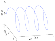
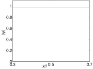
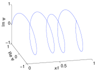
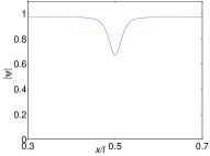
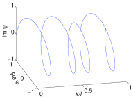
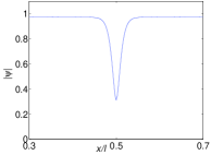
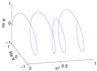
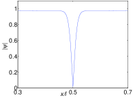
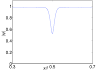
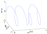
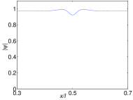
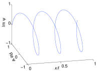
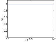
FIG. 1.: Minimal energy path from $\psi_{4}$ to $\psi_{3}$. Left column: $(Re\psi,Im\psi)$ as a function of $x$; Right column: $|\psi|$ as a function of $x$. The figures at the top and bottom correspond to $\psi_{4}$ and $\psi_{3}$, respectively. The third from the top is for the saddle point. In the fourth figure, $|\psi|$ reaches zero in the middle.

             

             

             

             

             

             

             

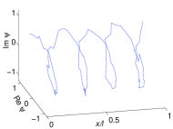
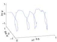
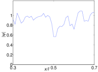
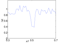
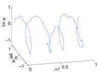
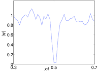
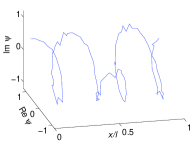
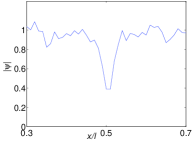
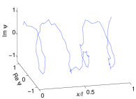
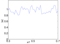
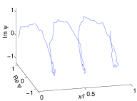
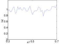
FIG. 2.: Transition pathway obtained from stochastic simulation, from $\psi_{4}$ to $\psi_{3}$ with thermal noise. Left column: $(Re\psi,Im\psi)$ as a function of $x$; Right column: $|\psi|$ as a function of $x$. The figures at the top and bottom correspond to $\psi_{4}$ and $\psi_{3}$, respectively. The third from the top is closest to the saddle point. In the fourth figure, $|\psi|$ reaches zero in the middle.

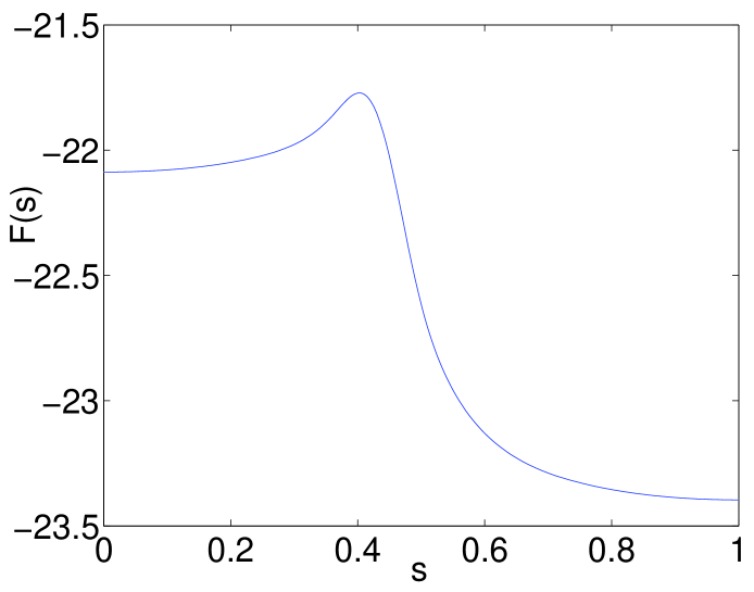
FIG. 3.: Scaled free energy $F$ evaluated along the MEP from $\psi_{4}$ to $\psi_{3}$, plotted as a function of the arc length $s$ in the $\psi(x)$-function space. The $\psi_{4}$ state is taken as the reference point where $s=0$.

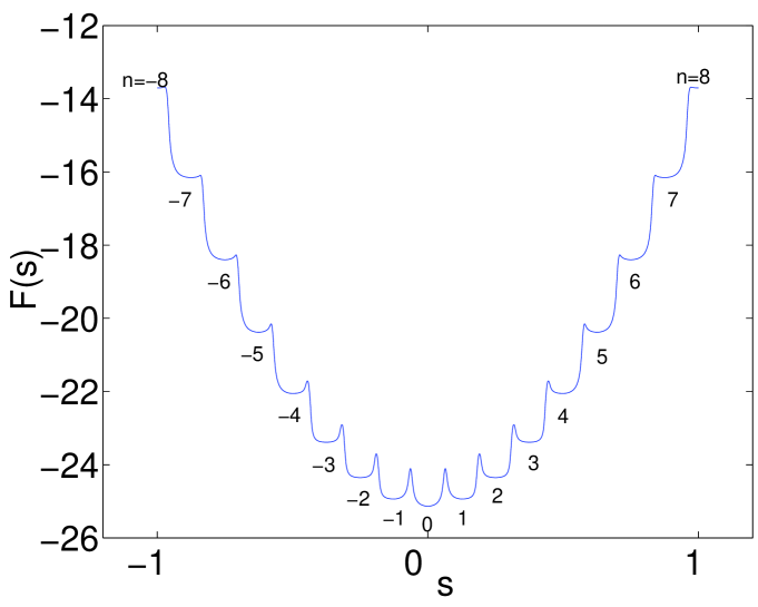
FIG. 4.: Scaled free energy $F$ evaluated along the MEPs connecting a sequence of metastable ($n\neq 0$) and stable ($n=0$) states, plotted as a function of the arc length $s$ in the $\psi(x)$-function space. The scaled system length is $l=32\pi$ and the zero-current state ($n=0$) is taken as the reference point where $F=-8\pi$ and $s=0$. The maximum $|n|$ allowed by $|k_{n}|<k_{c}$ is $9$. The plot here is up to $n=\pm 8$.

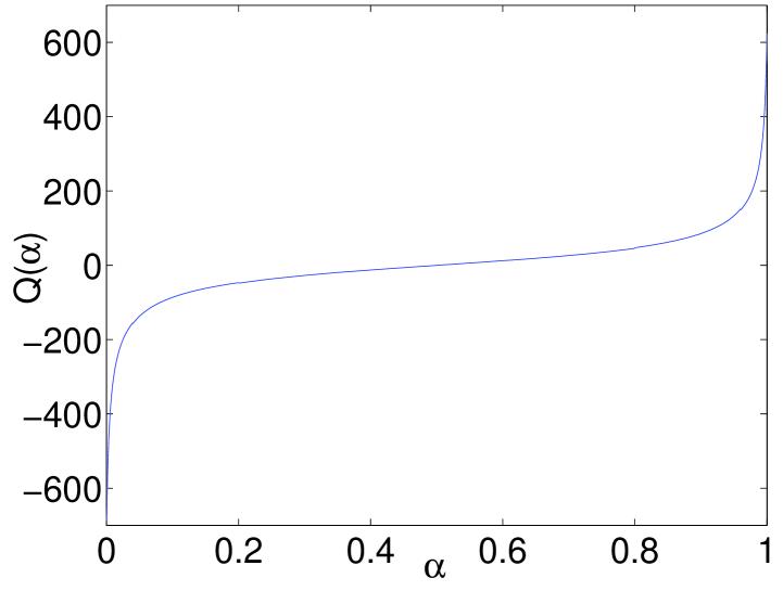
FIG. 5.: The expectation value $Q(\alpha)$ defined in Eq. (7), plotted as function of $\alpha$ in the interval $[0,1]$.

REFERENCES

- [1] W. A. Little, Phys. Rev. 156, 396 (1967).
- [2] J. S. Langer and V. Ambegaokar, Phys. Rev. 164, 498 (1967).
- [3] D. E. McCumber and B. I. Halperin, Phys. Rev. B 1, 1054 (1970).
- [4] A. Bezryadin, C. N. Lau, and M. Tinkham, Nature 404, 971 (2000); C. N. Lau, N. Markovic, M. Bockrath, A. Bezryadin, and M. Tinkham, Phys. Rev. Lett. 87, 217003 (2001).
- [5] W. E, W. Ren, and E. Vanden-Eijnden, Phys. Rev. B66, 052301 (2002).
- [6] W. E, W. Ren, and E. Vanden-Eijnden, J. Appl. Phys. 93, 2275 (2003).
- [7] W. E, W. Ren, and E. Vanden-Eijnden, String method for the study of rare events, unpublished.
- [8] W. Ren, Comm. Math. Sci. 1, 377 (2003).
- [9] H. A. Kramers, Physica 7, 284 (1940).
- [10] R. Landauer and J. A. Swanson, Phys. Rev. 121, 1668 (1961).
- [11] J. S. Langer, Phys. Rev. Lett. 21, 973 (1968).