An Empirical Tight-Binding Model for Titanium Phase Transformations

Abstract

For a previously published study of the titanium hcp ($\alpha$) to omega ($\omega$) transformation, a tight-binding model was developed for titanium that accurately reproduces the structural energies and electron eigenvalues from all-electron density-functional calculations. We use a fitting method that matches the correctly symmetrized wavefuctions of the tight-binding model to those of the density-functional calculations at high symmetry points. The structural energies, elastic constants, phonon spectra, and point-defect energies predicted by our tight-binding model agree with density-functional calculations and experiment. In addition, a modification to the functional form is implemented to overcome the “collapse problem” of tight-binding, necessary for phase transformation studies and molecular dynamics simulations. The accuracy, transferability and efficiency of the model makes it particularly well suited to understanding structural transformations in titanium.

I Introduction

Titanium is a useful starting material for many structural alloys;Leyens and Peters (2003) however, the formation of the high-pressure omega phase is known to lower toughness and ductility.Sikka et al. (1982) The atomistic mechanism of the transformation from the room temperature $\alpha$ phase (hcp) to the high-pressure $\omega$ was recently elucidated by Ref. [Trinkle et al., 2003]. The explication of the $\alpha$$\to$$\omega$ atomistic transformation relied on the comparison of approximate energy barriers for nearly 1000 different 6- and 12-atom pathways. That study required the use of an accurate and efficient interatomic potential model: in this case, a tight-binding model reparameterized using all-electron density-functional calculations.

After reparameterizing, we modify the functional form of tight-binding for small interatomic distances to overcome the collapse problem. This ensures that the potential is suitable for phase transition studies and molecular dynamics simulations. The collapse problem for tight-binding models is caused by unphysically large overlap at small distances creating a low energy binding state; by modifying the functional form using short-range splining, the collapse problem can be avoided. This paper provides the details of the model used in the previous phase transformation study of Ref. [Trinkle et al., 2003] and describes a general solution to the collapse problem.

Tight-binding is a parameterized electronic structure method for calculation of total energies and atomic forces for arbitrary structures. It is an empirical model that can reproduce density-functional results for a range of structures yet requires orders of magnitude less computational effort. The parameters of the model are determined by fitting to a database and the range of applicability is determined by comparison to structures not in the database. The end result is a model that balances three competing properties—efficiency, accuracy, and transferability—which make it applicable to a variety of important structures.

We fit our model to total energies and electron eigenvalues for several crystal structures over a range of volumes to produce a transferable model for the study of the $\alpha$$\to$$\omega$ transformation.Trinkle et al. (2003) Our fitting database is chosen to sample a large portion of the available phase space of parameters while constraining those parameters as much as possible. The resulting model accurately reproduces total energies, elastic constants, phonons, and point defects; all of which are necessary for transformation modeling. In addition, the functional forms are modified for small distances to overcome the unphysical collapse problem; this is necessary for phase transitions and molecular dynamics which sample small interatomic distances.

Section II describes tight-binding as a parameterized electronic structure method, the functional forms for titanium, the modifications for short distances, our fitting database and our method of optimization. Section III gives the optimized parameters, and tests our model against total energies, elastic constants, phonons, and point defect formation energies for $\alpha$, $\omega$, and bcc Ti. The point defect formation energies are used to compare our parameters to those of Mehl and PapaconstantopoulosMehl and Papaconstantopoulos (2002) and Rudin et al.,Rudin et al. (2004) and to demonstrate the efficacy of our modification of the short-range Hamiltonian and overlap functions.

II Methodology

II.1 Tight-binding formulation

Electronic structure methods separate the total energy of a crystal into an ionic contribution and an electronic contribution derived as the solution to a Hamiltonian problem. Treating electrons as non-interacting fermionic quasiparticles permits an appropriate one-particle solution.Kohn and Sham (1965) To numerically solve the electronic problem requires a set of basis functions $\phi_{i}$, in terms of which the matrix $H_{ij}$ of the Hamiltonian operator and overlap matrix $S_{ij}$ are

$$H_{ij}=\langle\phi_{i}|\hat{H}|\phi_{j}\rangle,S_{ij}=\langle\phi_{i}|\phi_{j}\rangle.$$

These matrices give the eigenvalue equation,

$$H\psi_{n}=\epsilon_{n}S\psi_{n},$$ (1)

where the electronic contribution to the total energy includes the term

$$2\sum_{\epsilon_{n}<E_{\text{F}}}\epsilon_{n},$$

with Fermi energy $E_{\text{F}}$. The Hamiltonian contains information about the wavefunction solutions themselves (e.g., density-functional theory). Typically, the wavefunctions must be found self-consistently, which increases the computational requirements.

In the tight-binding method, approximate Hamiltonian and overlap matrices are constructed by assuming atom-centered orbitals in a two-center approximation. This technique is related to the linear combination of atomic-like orbitals (LCAO) method, which uses a basis $\phi_{i}$ of solutions to the isolated atomic Schrödinger equation up to some energy and angular momentum quantum numbers $(nl)$: $\phi_{nlm}(\vec{r})=f_{nl}(|r|)Y_{lm}(\vec{r}/|r|)$. Tight-binding Hamiltonian and overlap functions are calculated independently of the local environment which increases efficiency but at the expense of transferability.

Empirical tight-binding eliminates explicit basis functions from the problem and parameterizes the Hamiltonian and overlap matrices in terms of simple two-center integrals.Slater and Koster (1954) The basis is chosen to be angular momentum solutions ${lm}$ up to some maximum $l$ value: For a maximum $l=1$ we use $s$, $p_{x}$, $p_{y}$ and $p_{z}$ as the basis functions; for a maximum of $l=2$, we add in the five $d$-orbitals $d_{xy}$, $d_{yz}$, $d_{zx}$, $d_{x^{2}-y^{2}}$ and $d_{3z^{2}-r^{2}}$. The Hamiltonian and overlap matrices are written as sums of parameterized functions $\bar{h}_{lm,l^{\prime}m^{\prime}}(\vec{r})$ and $\bar{s}_{lm,l^{\prime}m^{\prime}}(\vec{r})$ where $\vec{r}=\vec{R}_{i}-\vec{R}_{j}$ is the separation between two atoms $i$ and $j$. The two-center approximation allows these functions to be simplified further according to the angular momentum components of the basis.Slater and Koster (1954) For example, $\bar{h}_{p_{z},p_{z}}(\vec{r})$ separates into two symmetrized integrals

$$\bar{h}_{p_{z},p_{z}}(\vec{r})=h_{pp\sigma}(r)\cos^{2}\theta_{z}+h_{pp\pi}(r)\sin^{2}\theta_{z},$$

where $\theta_{z}$ is the angle between $\vec{r}$ and the $z$ axis. The higher rotational angular momentum integral $h_{pp\delta}(r)$ is zero because a $p$ orbital has a maximal azimuthal quantum number of 1 along the $z$ axis. The integrals $h_{pp\sigma}(r)$ and $h_{pp\pi}(r)$ are functions of only the distance of separation $r=|\vec{R}_{j}-\vec{R}_{j^{\prime}}|$. We write each Hamiltonian and overlap integral in these symmetrized functions; for a model with an $spd$ basis, there are ten integrals (for $h$ and $s$) to be determined: $(ss\sigma)$, $(sp\sigma)$, $(pp\sigma)$, $(pp\pi)$, $(sd\sigma)$, $(pd\sigma)$, $(pd\pi)$, $(dd\sigma)$, $(dd\pi)$, and $(dd\delta)$. The Hamiltonian and overlap matrices are then computed for an arbitrary atomic arrangement. The total energy of the system is given by the eigenvalues of the Eq. (1) $\epsilon_{n}$ and the ionic contribution:

$$E_{\mathrm{total}}=2\sum_{\epsilon_{n}<E_{\text{F}}}\epsilon_{n}+V(R_{\mathrm{nuclei}}),$$

where $V$ does not depend on the electronic states of the system.

We use functional forms developed at the U.S. Naval Research Laboratory (NRL) that do not use an explicit external pair potential but instead has environment dependent onsite energies.Mehl and Papaconstantopoulos (1996); Cohen et al. (1994); Yang et al. (1998) The onsite Hamiltonian elements $\epsilon_{s}$, $\epsilon_{p}$, and $\epsilon_{d}$ are not constants, but rather, depend on the distances of neighboring atoms to approximate three-body terms. The onsite energies $\epsilon_{l,i}$ are functions of the “local density” $\rho_{i}$ with four parameters

$$\epsilon_{l,i}=a_{l}+b_{l}\rho_{i}^{2/3}+c_{l}\rho_{i}^{4/3}+d_{l}\rho_{i}^{2},$$ (2)

where

$$\rho_{i}=\sum_{j\neq i}\exp(-\lambda^{2}r_{ij})f_{c}(r_{ij}).$$ (3)

The smooth cutoff function $f_{c}(r)$ is

$$f_{c}(r)=\left(1+\exp\left(\frac{r-R_{0}}{l_{0}}\right)\right)^{-1}.$$ (4)

The intersite functions $h_{ll^{\prime}m}(r)$ and $s_{ll^{\prime}m}(r)$ are given by three parameters each

$$\begin{split}h_{ll^{\prime}m}(r)&=(e_{ll^{\prime}m}+f_{ll^{\prime}m}r)\exp(-g^{2}_{ll^{\prime}m}r)f_{c}(r),\\ s_{ll^{\prime}m}(r)&=(\bar{e}_{ll^{\prime}m}+\bar{f}_{ll^{\prime}m}r)\exp(-\bar{g}^{2}_{ll^{\prime}m}r)f_{c}(r).\end{split}$$ (5)

The squared parameters $g_{ll^{\prime}m}$ and $\bar{g}_{ll^{\prime}m}$ guarantee the exponential terms to decay with increased distance.

The overlap and Hamiltonian functions have an unfortunate behavior for small distances $r$ which can lead to catastrophic failure in the Hamiltonian problem. The functional form in Eq. (5) is exponentially damped as $r$ grows; in reverse, this means that our intersite functions grow exponentially as $r$ becomes small. As $h$ or $s$ between two atoms grow in magnitude they increase the bonding between the two respective atoms; as $|s|\to 1$ the energy of the bond grows as $1/(1-|s|)$. When the bond energy grows, the bonding state is populated while the antibonding state is not; this results in a net attractive force between the two atoms. As the interatomic distance shrinks, the entire overlap matrix $S$ ceases to be positive-definite, and the Hamiltonian problem of Eqn. (1) is no longer solvable. This causes the “collapse problem” in molecular dynamics: two atoms come close to each other and see a large attractive force that pulls them towards each other until $S$ is not positive-definite. In actuality, the Hamiltonian problem is not meaningful even before $S$ is not positive-definite, because the model predicts a bond with an unphysically low energy. In a real material, the growth in bonding is counteracted by Coulumb repulsion: a two-electron term that is not included in the tight-binding formalism.

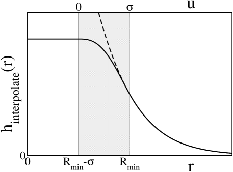
Figure 1: Interpolated intersite function with short-range spline. The parameterized function $h(r)$ grows exponentially as $r$ approaches zero, though the function is only sampled in the fitting database down to $R_{\text{min}}$. At $r=R_{\text{min}}$, we replace the function with a quartic spline that matches the value, first and second derivatives at $R_{\text{min}}$; the dashed curve shows the growth of the original function. The spline smoothly goes to a constant value in a width of $\sigma$. Only one adjustable parameter, $\sigma$, is added to the entire fitting database, as $\sigma$ is the same for all functions.

Short-range splining. To resolve this, we modify the intersite functions to keep the overlap matrix $S$ positive definite. Because our fitting database includes only interatomic distances larger than some minimum distance $R_{\text{min}}$, the functional form is guaranteed to be correct only for $r>R_{\text{min}}$. Below $R_{\text{min}}$, we smoothly interpolate both $h_{ll^{\prime}m}(r)$ and $s_{ll^{\prime}m}(r)$ to a constant value. The interpolation is performed with a quartic spline, from $r=R_{\text{min}}$ down to $r=R_{\text{min}}-\sigma$; below $R_{\text{min}}-\sigma$, the function takes on a constant value. We choose spline values to enforce continuity of value and the first and second derivatives; the final functions for both $h_{ll^{\prime}m}(r)$ and $s_{ll^{\prime}m}(r)$ are

$$h_{\text{inter.}}(r)=\begin{cases}h(r)&:r>R_{\text{min}},\\ h_{\text{spline}}(0)&:r<R_{\text{min}}-\sigma,\\ h_{\text{spline}}(r-R_{\text{min}}+\sigma)&:\mathrm{otherwise},\\ \end{cases}$$ (6)

where

$$h_{\text{spline}}(u)=h_{0}-\frac{1}{2}\sigma h^{\prime}_{0}+\frac{1}{12}\sigma^{2}h^{\prime\prime}_{0}+\left(\sigma h^{\prime}_{0}-\frac{1}{3}\sigma^{2}h^{\prime\prime}_{0}\right)\frac{u^{3}}{\sigma^{3}}\\ +\left(-\frac{1}{2}\sigma h^{\prime}_{0}+\frac{1}{4}\sigma^{2}h^{\prime\prime}_{0}\right)\frac{u^{4}}{\sigma^{4}},$$ (7)

for $u$ in $[0,\sigma]$, and $h_{0}$, $h^{\prime}_{0}$, and $h^{\prime\prime}_{0}$ are the value, first, and second derivative of $h(r)$ at $R_{\text{min}}$. Figure 1 shows this interpolation schematically. While we smoothly interpolate $h_{ll^{\prime}m}$ and $s_{ll^{\prime}m}$, we retain the environment-dependent onsite terms; this has the effect of reducing the strength of bonding while the onsite energy continues to grow—effectively producing a pair repulsion between atoms at small distances.

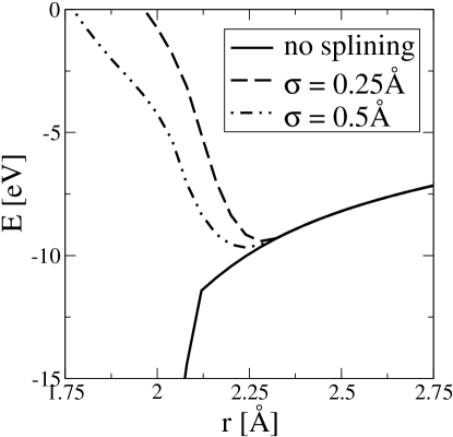
Figure 2: Energy of Ti dimer calculated with tight-binding using short-range splining. Without any short-range splining, the overlap matrix becomes artificially large, creating a bonding state with very low energy at small distances; at 1.92Å, the tight-binding dimer Hamiltonian problem becomes unsolvable. As described in the text, by short-range splining of the Hamiltonian and overlap functions, the model is stable and becomes repulsive at small distances.

Figure 2 illustrates the collapse problem for the Ti dimer and how short-range splining stabilizes the model for small distances. As the distance between the two atoms decreases, a bonding state with an artificially low energy decreases the dimer energy. The precipitous drop in the energy of this bonding state is due to an increase in the overlap; at 1.92Å, the overlap matrix becomes non-positive definite, and the eigenproblem is no longer solvable. A $\sigma$ value of 0.5Å or 0.25Å makes the dimer stable; this is necessary but not sufficient to solve the collapse problem for all cases.

Our parameterization has 74 parameters to be optimized, plus 3 fixed parameters. The cutoff function $f_{c}(r)$ has two fixed parameters $R_{0}$ and $l_{0}$, while the minimum distance $R_{\text{min}}$ is set by the database. There are 10 Hamiltonian and 10 overlap functions, each with 3 parameters for a total of 60 parameters. The 3 onsite energy functions have 4 parameters each, and a single parameter $\lambda$ for the density gives 13 parameters. Finally, the short-range spline range parameter $\sigma$ is determined using the dimer, and testing with molecular dynamic calculations and defect relaxations.

II.2 Fitting database

We compile a database of electronic structure calculations of several crystal structures using full-potential linearized augmented plane wave (FLAPW) calculationsSingh (1994) with the wien97 program suite.Blaha et al. (1999) We use the generalized gradient approximation (GGA) for the exchange-correlation energy.Perdew et al. (1996) The sphere radius is $R_{\text{MT}}=2.0\text{~{}bohr}=1.06\text{~{}\AA}$; there is a negligible charge leakage of $10^{-8}$ electrons. The planewave cutoff $K_{\text{max}}$ is given by $R_{\text{MT}}K_{\text{max}}=9$; this corresponds to an energy cutoff of 275 eV. The energy cutoff is not as large as required in a typical pseudopotential calculation because the planewaves are only used in the interstitial regions away from atom centers. The charge density is expanded in a Fourier series; the largest magnitude vector in the expansion $G_{\text{max}}$ is 18 bohr^-1 (34 Å^-1). Local orbitals are used for the $s$, $p$, and $d$ solutions inside the spheres.Singh (1994) Our core configuration is Mg with semi-core $3p$ states represented by the local $p$ orbitals; our $4s$, $3d$, and $4p$ states are the valence orbitals. A Fermi-Dirac smearing of 20 mRyd (272 meV) is used to calculate the total energy.

Table 1: Crystal structures used in tight-binding fitting database. Five different crystals structures are used, with five volumes for each of the cubic crystal structures. The lattice constant a₀, volume per atom, and nearest neighbor distance and multiplicity for each structure is listed. The equilibrium lattice constant for each structure is marked with an asterisk. The same $k$-point mesh is used for all volumes of a given structure, and is constructed using the prescription of Ref. [Chadi and Cohen, 1973; Monkhorst and Pack, 1976]. The smallest distance to appear in this fitting database is $R_{\text{min}}=2.350\text{~{}\AA}$.

Structure	a0 (Å)	V/atom (Å3)	nn (Å)	$k$-point mesh
bcc	2.887	12.03	2.500 $\times 8$	shifted $5\times 5\times 5$
	3.060	14.32	2.650 $\times 8$	(44 points)
	3.281∗	17.66	2.841 $\times 8$
	3.406	19.76	2.950 $\times 8$
	3.579	22.93	3.100 $\times 8$
fcc	3.747	13.16	2.650 $\times 12$	unshifted $5\times 5\times 5$
	3.960	15.52	2.800 $\times 12$	(47 points)
	4.127∗	17.57	2.919 $\times 12$
	4.384	21.06	3.100 $\times 12$
	4.596	24.27	3.250 $\times 12$
sc	2.350	12.98	2.350 $\times 6$	shifted $5\times 5\times 5$
	2.500	15.62	2.500 $\times 6$	(35 points)
	2.645∗	18.50	2.645 $\times 6$
	2.800	21.95	2.800 $\times 6$
	2.950	25.67	2.950 $\times 6$
$\alpha$	2.952∗	17.69	2.952 $\times 12$	unshifted $5\times 5\times 2$
	($c/a=1.588$)			(42 points)
$\omega$	4.600∗	17.23	2.656 $\times 3$	unshifted $3\times 3\times 4$
	($c/a=0.613$)			(35 points)
	∗ FLAPW equilibrium lattice constant

Table 1 shows a summary of the fitting database; it consists of the total energies and eigenvalues on a $k$-point grid for several crystal structures. Five structures are used: simple cubic (sc), body-centered cubic (bcc), face-centered cubic (fcc), hexagonal closed-packed ($\alpha$), and omega ($\omega$). The three cubic structures are calculated over a range of volumes, while the hexagonal structures are calculated only at FLAPW equilibrium volumes and $c/a$ ratios. The eigenvalues in each structure are each shifted by a constant amount so that the sum of the occupied bands (smeared by 272 meV) is the total energy. We calculate the 9 lowest bands per atom above the semicore $3p$ states; these represent the $4s$, $3d$ and $4p$ states both below and above the Fermi level. We use the lowest 6 bands at each $k$-point for fitting the cubic structures, 9 bands for $\alpha$, and 12 bands for $\omega$.

In addition to eigenvalues on a regular grid, we include eigenvalues at high symmetry points and directions in the Brillouin zone to aid in fitting.Papaconstantopoulos (1986); Jones and Albers (2002) For the three cubic structures, we calculate the eigenvalues at several high-symmetry points and directions (10 for bcc and sc, and 12 for fcc) and then decompose the electronic wavefunctions in terms of the symmetry character of the eigenvalues.Cornwell (1969) Again, we use the lowest 6 states for the high-symmetry points. We are careful not to fit too many eigenvalues at high-symmetry points, since the lowest 9 bands in the GGA band structure may not correspond to those predicted in our $spd$ basis.

Because our fit includes the electron eigenvalues, we expect our model to reproduce both total energies and energy derivatives. Phonons and elastic constants can be written in terms of the forces on atoms due to small displacements; the Hellman-Feynman theorem relates the force on an atom $R_{i}$ to the eigenvalues as

$$F_{i}=-2\sum_{\varepsilon_{n}<E_{\text{F}}}\langle\psi_{n}|\frac{\partial\hat{H}}{\partial R_{i}}|\psi_{n}\rangle.$$

Thus, the electron eigenvalues of the bulk crystal contain information about phonons and elastic constants.

II.3 Optimization of parameters

The parameters are optimized to minimize the mean squared error. We use the non-linear least-squares minimization method of Levenberg-Marquardt with a numerical Jacobian.Marquardt (1963) We weight each $k$-point by unity, and the resulting total energy by 200; accordingly the total energies are weighted approximately the same as the $k$-point data. We initialize our parameters using the Hamiltonian and overlap values for Ti from Ref. [Papaconstantopoulos, 1986] adapted to our functional form. We then fit only the environment-dependent onsite terms to the band-structure of the cubic elements. After an initial fit is found, we include the hopping terms in the optimization. We proceed using only the cubic band structure, then the cubic band structure and total energies, and finally all structures and energies. After a new minimum is found, we check each function to see if the minimization has made the exponential term $g_{(ll^{\prime}m)}$ too large; this corresponds to making the entire function approximately zero over the sampled range of $r$ values. We remedy this by resetting the $e$, $f$, and $g$ parameters to 0, 0, and 0.5. Several fitting runs are performed until the entire fit set is accurately reproduced.

III Results

III.1 Parameters and fitting residuals

Table 2 lists the parameters of the optimized tight-binding model. Figure 3 shows the hopping integrals $h_{(ll^{\prime}m)}(r)$ and $s_{(ll^{\prime}m)}(r)$ for a range of volumes; the $R_{\text{min}}$ in the database is 2.35 Å, and we interpolate each function to a constant value below $R_{\text{min}}$. Finally, Figure 4 shows the environment-dependent onsite energies as a function of volume for an hcp crystal with $c/a=1.588$.

Table 2: Tight-binding parameterization for titanium. The onsite parameters are given for the $s$, $p$, and $d$ orbitals. Each term is density dependent; the parameter in the density dependence is $\lambda$. The cutoff function has fixed parameters $R_{0}$ and $l_{0}$. Next, the intersite Hamiltonian and overlap elements are given for each of the 10 symmetrized $(ll^{\prime}m)$ combinations. Below $R_{\text{min}}$, each intersite function is smoothly interpolated to a constant value over the range $\sigma$.

	$a_{l}$ (eV)	$b_{l}$ (eV)	$c_{l}$ (eV)	$d_{l}$ (eV)
$s$:	$-3.272\times 10^{{0}}$	$3.714\times 10^{{2}}$	$8.029\times 10^{{3}}$	$7.879\times 10^{{4}}$
$p$:	$4.974\times 10^{{0}}$	$3.747\times 10^{{1}}$	$-1.874\times 10^{{3}}$	$2.721\times 10^{{4}}$
$d$:	$3.632\times 10^{{-1}}$	$3.238\times 10^{{1}}$	$8.877\times 10^{{1}}$	$9.355\times 10^{{2}}$
$\epsilon_{l,i}=a_{l}+b_{l}\rho_{i}^{2/3}+c_{l}\rho_{i}^{4/3}+d_{l}\rho_{i}^{2}$				(2)

$$\rho_{i}=\sum_{j\neq i}\exp(-\lambda^{2}r_{ij})f_{c}(r_{ij})\text{\,:\quad} \lambda^{2}=\left(0.3620\text{~{}\AA}\right)^{-1}$$ (3)

$$f_{c}(r)=\left(1+\exp\left(\frac{r-R_{0}}{l_{0}}\right)\right)^{-1}\text{\,:\quad} \begin{array}[]{c}R_{0}=6.615\text{~{}\AA}\\ l_{0}=0.2646\text{~{}\AA}\end{array}$$ (4)

		$e_{(ll^{\prime}m)}$	$f_{(ll^{\prime}m)}$	1/$g_{(ll^{\prime}m)}^{2}$
$ss\sigma$:	h=	$-1.086\times 10^{{2}}$ eV	$-3.900\times 10^{{3}}$ eV/Å	$0.3277$ Å
	s=	$9.277$	$-2.624$ Å-1	$0.8357$ Å
$sp\sigma$:	h=	$-1.793\times 10^{{3}}$ eV	$8.066\times 10^{{2}}$ eV/Å	$0.4926$ Å
	s=	$-11.81$	$0.02523$ Å-1	$0.5993$ Å
$pp\sigma$:	h=	$-4.865\times 10^{{2}}$ eV	$1.816\times 10^{{2}}$ eV/Å	$0.6929$ Å
	s=	$0.08093$	$-1.351$ Å-1	$1.036$ Å
$pp\pi$:	h=	$1.202\times 10^{{1}}$ eV	$-8.252\times 10^{{0}}$ eV/Å	$0.8925$ Å
	s=	$4.478$	$-0.2899$ Å-1	$0.8026$ Å
$sd\sigma$:	h=	$-5.537\times 10^{{2}}$ eV	$3.096\times 10^{{2}}$ eV/Å	$0.4772$ Å
	s=	$-4.331$	$-5.085$ Å-1	$0.4498$ Å
$pd\sigma$:	h=	$-2.338\times 10^{{2}}$ eV	$9.994\times 10^{{1}}$ eV/Å	$0.6321$ Å
	s=	$0.02557$	$-3.383$ Å-1	$0.5728$ Å
$pd\pi$:	h=	$-4.979\times 10^{{0}}$ eV	$7.855\times 10^{{-1}}$ eV/Å	$1.617$ Å
	s=	$0.1943$	$2.308$ Å-1	$0.5882$ Å
$dd\sigma$:	h=	$1.706\times 10^{{2}}$ eV	$-1.150\times 10^{{2}}$ eV/Å	$0.5266$ Å
	s=	$-0.9905$	$0.7605$ Å-1	$0.7990$ Å
$dd\pi$:	h=	$9.920\times 10^{{0}}$ eV	$3.538\times 10^{{1}}$ eV/Å	$0.5366$ Å
	s=	$-1.490$	$-1.498$ Å-1	$0.5213$ Å
$dd\delta$:	h=	$1.109\times 10^{{3}}$ eV	$-6.205\times 10^{{2}}$ eV/Å	$0.3340$ Å
	s=	$15.58$	$-5.276$ Å-1	$0.4412$ Å
$\{h,s\}_{(ll^{\prime}m)}(r)=\left(e_{(ll^{\prime}m)}+f_{(llm^{\prime})}r\right)\exp(-g^{2}_{(ll^{\prime}m)}r)f_{c}(r)$ (5)
$R_{\text{min}}=2.350\text{~{}\AA},\quad\sigma=0.265\text{~{}\AA}$				(6)

To use the potential for phase-transformation studies, $\sigma$ was determined by testing the stability of (1) the dimer, (2) molecular dynamics runs, and (3) defect relaxations. While the lowest energy pathways studied by Ref. [Trinkle et al., 2003] have distances of closest approach of 2.6 Å, there were possible pathways where atoms approached within 2.3 Å of each other. Without short-range splining, calculations of energies of structures with distances below our $R_{\text{min}}$ value can become problematic. Initially, a $\sigma$ value of 0.529 Å was chosen based on the dimer; however, defect relaxation calculations showed that a value of 0.265 Å was necessary to ensure stability for some of the point defects.

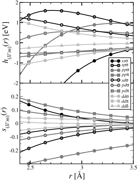
Figure 3: Tight-binding intersite Hamiltonian and overlap functions. The parameterized hopping integrals are shown for distances from 2.4 Å to 3.5 Å. The $R_{\text{min}}$ in the fit is 2.35 Å; below this, these functions are smoothly interpolated to a constant value. Circles represent $\sigma$ integrals, squares $\pi$ integrals, and triangles $\delta$ integrals; black is for $s$, dark gray for $p$, and light gray for $d$.

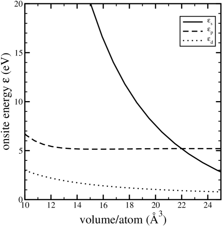
Figure 4: Tight-binding onsite energy terms for hcp structure. The onsite energies are environment dependent in our model; we show the variation with respect to the volume of an hcp crystal with $c/a=1.588$. The low volume of 10 Å³ has a lattice constant of 2.44 Å, and the high volume of 25 Å³ has a lattice constant of 3.31 Å. The equilibrium hcp volume is 17.56 Å³.

Table 3: Fitting errors in total energy and $k$-points for tight-binding model. For each structure, we report the absolute error in the total energy (first line) and the RMS error in all $k$-point energies in the fit set (second line). The total energy errors are on the order of 1 meV, while the RMS band-structure errors are on the order of 100 meV.

	low volume	equilibrium	high volume
bcc	1.64 meV	0.957 meV	4.31 meV
	200 meV	104 meV	110 meV
fcc	–1.79 meV	1.25 meV	–0.821 meV
	136 meV	87.1 meV	114 meV
sc	–0.0190 meV	–0.115 meV	–1.60 meV
	435 meV	195 meV	140 meV
$\alpha$		–1.66 meV
		69.1 meV
$\omega$		–0.00993 meV
		67.9 meV

Table 3 lists the errors in our tight-binding model with respect to the fitting database. Our average total energy errors are approximately 1 meV; root-mean square errors in the $k$-point energies are approximately 100 meV. The tight-binding parameterization adequately reproduces the database energetics. To test transferability, we compare to properties outside of this database.

III.2 Total energies

Figure 5: Comparison of tight-binding energy as a function of volume for $\alpha$ and $\omega$ with first principles data. The two filled points were included in the fit; the lines are FLAPW total energies. Our tight-binding model reproduces the fit data—slightly lower ground-state energy and equilibrium volume for $\omega$—and the equation of state of the full-potential calculations.

Figure 5 shows the tight-binding total energy as a function of volume for $\alpha$ and $\omega$. These curves were not included in the fitting database; only the two points indicated. We reproduce both the slightly lower energy of $\omega$ over $\alpha$ predicted by pseudopotential methodsTrinkle et al. (2003) and FLAPW calculations, as well as the slightly lower equilibrium volume of $\omega$. The three cubic structures were included in the fit and have errors on the order of 3 meV/atom (c.f., Table 3). This shows a wide range of applicability for our model under pressure.

III.3 Elastic constants and phonons

Table 4: Lattice parameters and elastic constants in units of GPa for $\alpha$, $\omega$, and bcc Ti from tight-binding, GGA, and experiment. GGA corresponds to the elastic constants found using vasp.Kresse and Hafner (1993); Kresse and Furthmüller (1996) The experimental $\alpha$ elastic constants are measured at 4K,Simmons and Wang (1971) and the bcc elastic constants at 1238K.Petry et al. (1991) Our tight-binding model reproduces the GGA elastic constant combinations that preserve the symmetry of the structure (e.g., $C_{11}+C_{12}$), but has larger error with those that break it (e.g., $C_{44}$). The deviation between the bcc experimental elastic constants and our calculations is due to the high temperature needed to stabilize the bcc structure in Ti.

	a (Å)	c (Å)	$C_{11}$	$C_{12}$	$C_{13}$	$C_{33}$	$C_{44}$
	Tight-binding
$\alpha$	2.94	4.71	155	91	79	173	65
$\omega$	4.58	2.84	184	90	52	261	100
bcc	3.27	—	87	112	—	—	31
	GGA
$\alpha$	2.95	4.68	172	82	75	190	45
$\omega$	4.59	2.84	194	81	54	245	54
bcc	3.26	—	95	110	—	—	42
	Experiment
$\alpha$	2.95	4.68	176	87	68	191	51
bcc	3.31	—	134	110	—	—	36

Table 4 shows the equilibrium lattice constants and elastic constants for $\alpha$, $\omega$, and bcc for our tight-binding model. The GGA numbers correspond to the elastic constants found using vasp.Kresse and Hafner (1993); Kresse and Furthmüller (1996) Elastic constant combinations which do not break symmetry such as $C_{11}+C_{12}$, $C_{13}$, $C_{33}$ in the hexagonal crystals, and $C_{11}+2C_{12}$ in bcc are reproduced within approximately 10%. However, the symmetry breaking elastic constant combinations such as $C_{11}-C_{12}$ and $C_{44}$ have larger errors. It is worth noting that none of this data, except for the bulk modulus of bcc, appears in any form in the fitting database; the agreement is a consequence of reproducing the electron eigenvalues.

We calculate phonons using the direct-force method.Kunc and Martin (1982); Wei and Chou (1992); Frank et al. (1995); Parlinski et al. (1997) We calculate the forces on all atoms in a supercell where one atom at the origin is displaced by a small amount. The numerical derivative of the forces with respect to the displacement distance approximates the force constants folded with the translational symmetry of the supercells. The Fourier transform of the force constants gives the dynamical matrix, and its eigenvalues give the phonon frequencies.Ashcroft and Mermin (1976) For $q$ vectors commensurate with the supercell, the phonon frequencies are exact; for incommensurate $q$ vectors, the calculated phonons are a Fourier interpolation between exact values. Our supercells are $4\times 4\times 3$ for $\alpha$, $3\times 3\times 4$ for $\omega$, and $4\times 4\times 4$ simple cubic cell for bcc; in all cases, a $2\times 2\times 2$ $k$-point mesh is used in the supercell.

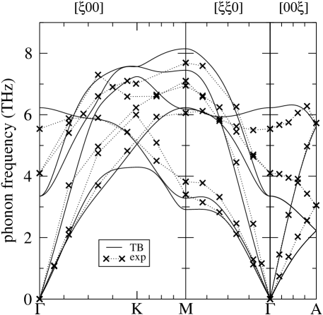
Figure 6: Comparison of tight-binding phonons for the $\alpha$ phase with experimental phonon data. The crosses are the experimental phonon frequencies at 295K.Stassis et al. (1979) The deviation from the experimental values at small $q$ corresponds to the mismatch in the $\alpha$ elastic constants. Our tight-binding model does well for the high-energy optical and acoustic branches which are important for modeling the $\alpha$$\to$$\omega$ transformation.

Figure 7: Predicted $\omega$ phonons from tight-binding. As expected from the $c/a$ ratio of 0.620, the phonon modes are stiffer along the $[00\xi]$ direction than the basal plane directions $[\xi 00]$ and $[0\xi 0]$.

Figure 8: Predicted bcc phonons from tight-binding. At $T=0$, the bcc phase in Ti is unstable, as shown by the imaginary phonon frequencies. The dip in the $[\xi\xi\xi]$ branch is near the L-$\frac{2}{3}[111]$ phonon, which corresponds to the bcc$\to$$\omega$ transformation pathway. The imaginary phonon for T-$[011]$ corresponds to the bcc$\to$$\alpha$ transformation mechanism.Burgers (1934)

Figures 6, 7, and 8 are the predicted phonon dispersions for our tight-binding model, calculated at the equilibrium volumes for each structure. The $\alpha$ phonons match the experimental values well for the high energy phonons optical and acoustic branches; these are important for modeling the shuffle during martensitic transformation. The deviation from experiment for small $q$ corresponds to our mismatch in elastic constants. The $\omega$ phonons are expectedly stiffer along the $c$ axis than in the basal plane due to the low $c/a$ ratio. The bcc phonons show phonon instabilities corresponding to the bcc$\to$$\omega$ transformation (L-$\frac{2}{3}[111]$ phonon) and the bcc$\to$$\alpha$ transformation (T-$[011]$ branch).Burgers (1934)

III.4 Point defects

Table 5 shows the formation energies of point defects for $\alpha$ and $\omega$ at the equilibrium volumes for our tight-binding model. All $\alpha$ calculations are performed with a $4\times 4\times 3$ (96 atom) supercell and all $\omega$ with a $3\times 3\times 4$ (108 atom) supercell. No point defect information is included in the initial fit; we reproduce the GGA formation energies for all of the point defects considered. This indicates that our tight-binding model is applicable to the study of the $\alpha$$\to$$\omega$ transformation path, where atoms move out of their equilibrium configurations and often close to one another.

Table 5: Point defect energies in eV for $\alpha$ and $\omega$ Ti from tight-binding for different parameterizations. GGA refers to the defect formation energies calculated with vasp; TB to the parameterization in this work; NRL to the parameterization by Mehl and Papaconstantopoulos;Mehl and Papaconstantopoulos (2002) and LANL to the parameterization by Rudin et al.Rudin et al. (2004) NN refers to the distance of closest approach for two atoms in each defect in TB. The formation energies are calculated after relaxation. The defects marked coll. fell victim to the “collapse problem” during relaxation. The $\alpha$-tetrahedral site is unstable, relaxing to form a dumbbell along the $[0001]$ direction in GGA. The $\omega$-hexahedral site is very close to the $\omega$-tetrahedral site.Hennig et al. (2005) Many of the interstitial defects sample small distances, requiring the use of short-range splining to stabilize the defects.

Defect	GGA	TB	NRL	LANL	NN [Å]
$\alpha$ defects
Octahedral	2.58	2.89	1.31	2.55	2.50 Å
Tetrahedral	unstable
Dumbbell-$[0001]$	2.87	2.81	1.81	coll.	2.18 Å
Vacancy	2.03	1.88	1.51	1.92	2.83 Å
Divacancy-AB	3.92	3.83	3.73	3.68	2.81 Å
$\omega$ defects
Octahedral	3.76	4.11	3.20	3.67	2.30 Å
Tetrahedral	3.50	3.58	2.86	coll.	2.21 Å
Hexahedral	3.49	3.86	2.88	4.37	2.28 Å
Vacancy-A	2.92	2.85	2.99	3.25	2.60 Å
Vacancy-B	1.57	1.34	1.01	1.90	2.62 Å

The formation energies of point defects shows some improvement of our model over two existing models.Mehl and Papaconstantopoulos (2002); Rudin et al. (2004) The potential by Rudin et al. uses the same functional forms as our potential without short-range splining for hopping and overlap functions; Mehl and Papaconstantopoulos use the same onsite function form, but adds additional quadratic parameters to the hopping and overlap functions in Eqn. (5). All three potentials use the same onsite functional forms. For all three potentials, the binding energies versus volume, elastic constants, and phonons are similar, though Rudin’s more accurately captures the low frequency $\alpha$ phonons. However, point defect formation energies are better predicted by our tight-binding parameterization.

The short distances sampled by the point defects emphasize the need for short-range splining of both the overlap and Hamiltonian functions. The collapse of two defects in Rudin et al.’s model is due to the growth of the overlap matrices; the lower energies predicted by Mehl and Papaconstantopoulus could be due to overly large overlap elements at short-distances as well. Interstitial defects, like phase transformation pathways, can sample interatomic distances smaller than the smallest distance included in the fitting database; without short-range splining, this can lead to artificially lower energies, or even collapse. Without short-range splining, all three tight-binding parameterizations fail for the Ti dimer at small distances: 1.92 Å for this work, 1.76Å for Mehl and Papaconstantopoulos, and 1.28 Å for Rudin et al. The use of short-range splines provides a solution to the collapse problem for non-orthogonal tight-binding models.

IV Conclusion

We present an accurate and transferable tight-binding model with parameters determined by density-functional calculations. It reproduces structural energies with pressure, elastic constants, phonons, and point defect energies. By fixing the short-range behavior of the potential, point defects can be accurately computed, which allows the calculation of energy barriers for phase transformation pathways. The wide range of applicability makes it particularly well suited to the study of martensitic phase transformations, such as $\alpha$$\to$$\omega$;Trinkle et al. (2003) and short-range splines represent a solution to the potential collapse problem of non-orthogonal tight-binding models.