Computer simulation of quantum melting in hydrogen clusters

Abstract

We introduce a new criterion—based on multipole dynamical correlations calculated within Reptation Quantum Monte Carlo—to discriminate between a melting vs. freezing behavior in quantum clusters. This criterion is applied to small clusters of para-hydrogen molecules (both pristine and doped with a CO cromophore), for cluster sizes around 12 molecules. This is a magic size at which para-hydrogen clusters display an icosahedral structure and a large stability. In spite of the similar geometric structure of CO@($p$H₂)₁₂ and ($p$H₂)₁₃, the first system has a rigid, crystalline, behavior, while the second behaves more like a superfluid (or, possibly, a supersolid).

Understanding the dynamics of quantum many-body systems is one of the major challenges presently set to theoretical and computational condensed-matter physicists. The combination of density-functional theory with molecular dynamics realized 20 years ago by Car and Parrinello CarParr opened the way to the study of the dynamics of quantum driven classical systems (i.e. of atomic systems whose dynamics is essentially classical, but driven by quantum-mechanical forces). The development of density-functional perturbation theory has allowed for a systematic calculation of the low-lying quantum excited states of these same systems in the harmonic approximation BGT . Quantum Monte Carlo methods, on the other hand, have been very successful in describing the ground-state and finite-temperature properties of interacting bosons RMP-Ceperley and of lattice models of strongly interacting fermions fermion-lattice , and they promise a similar success in the study of chemical systems in the near future QMC-RMP . In spite of all these progresses, the ability to calculate in a reliable way the properties of the excited states of interacting quantum systems remains a largely unachieved goal. Recent advances in the quantum Monte Carlo methodology have partially changed this scenario, at least in what concerns systems whose ground-state wave-function is positive (i.e. bosons) and whose low-lying energy spectrum is dominated by few excited states, which is the typical situation for superfluids noantri ; genova . Thanks to these advances, it is now possible to calculate the low-lying excitation spectrum of clusters of up to a few tens ⁴He atoms, possibly doped with some cromophore molecules which are experimentally used as spectroscopic probes of the dynamical and superfluid properties of the droplet.

Molecular hydrogen, in its nuclear-spin realization called para-hydrogen ($p$H₂, $I=J=0$), is the only substance occurring in nature, other than ⁴He, which can possibly exhibit the phenomenon of superfluidity at (not too) low temperature ginzburg . In spite of the lighter mass with respect to ⁴He, the intermolecular potential is so much stronger that the estimated value of the $\lambda$-transition temperature ($\approx 2\rm^{\circ}K$) is much lower than the observed triple-point temperature ($13.96\rm^{\circ}K$). For this reason, much attention has been and is being paid to those confined geometries (such as clusters ceperley_h2 ; toennies-science ; levi ; whaley-h2 ; toennies-PRL or films gordillo-ceperley ; boninsegni ) which may hinder crystallization and make superfluidity (or what remains of it in these geometries) observable in $p$H₂. Discriminating between a melting vs. freezing behavior in a finite system is a subtle issue which requires a careful consideration of the dynamical evolution of the system. In this paper we propose a strategy to cope with this problem, based on Reptation Quantum Monte Carlo (RQMC), a method that we developed a while ago to deal with dynamical correlations in systems of interacting bosons noantri . As a (still very preliminary) application, we show how using suitable (imaginary-) time correlation functions it is easy (and fun!) to discriminate between the melting vs. freezing behavior of small $p$H₂ clusters—with or without a CO molecule solvated in them—for sizes close to $n=13$, a magic number which favors crystallization.

Reptation Quantum Monte Carlo

The dynamics of classical stochastic processes bears close similarities with the time evolution of quantum systems in imaginary time. These similarities—together with the fact that every system tends towards the ground state at large imaginary times—lay at the basis of many quantum Monte Carlo methods which sample ground state properties from the equilibrium properties of a suitably defined classical random walk. Comparatively minor attention has been paid to the dynamical properties of the random walks used in quantum simulations. In this section we show how a careful exploitation of these similarities can be used to estimate the dynamical properties of strongly interacting boson fluids.

Most ground-state Monte Carlo techniques are based on the property that the imaginary-time evolution of (almost) any trial wave-function, $\Phi_{0}$, in the infinite-time limit tends to the ground state, $\Psi_{0}$. As a consequence, the ground-state energy can be expressed as:

$$E_{0} = \lim_{\tau\to\infty}{\langle\Phi_{0}|H{\rm e}^{-H\tau}|\Phi_{0}\rangle\over\langle\Phi_{0}|{\rm e}^{-H\tau}|\Phi_{0}\rangle}$$ (1)

$$= -\lim_{\tau\to\infty}{d\over d\tau}\log{\cal Z}_{0}$$ (2)

$$= -\lim_{\tau\to\infty}{1\over\tau}\log{\cal Z}_{0},$$ (3)

where $H=-{\partial^{2}\over\partial x^{2}}+V(x)$ is the Hamiltonian of the system and ${\cal Z}_{0}=\langle\Phi_{0}|{\rm e}^{-H\tau}|\Phi_{0}\rangle$. If ${\cal Z}_{0}$ is thought as the partition function of an auxiliary, fictitious, system, then Eqs. (2) and (3) express the free and internal energies of this system in the zero-temperature limit. By using Eq. (3), ground-state expectation values of static operators and generalized susceptibilities can be expressed as first and second logarithmic derivatives of ${\cal Z}_{0}$ with respect to the strength of a suitably chosen perturbation to the Hamiltonian noantri .

A link with the theory of stochastic processes can be established by splitting the Hamiltonian as:

$$H={\cal H}+{\cal E}(x),$$ (4)

where ${\cal H}=-{\partial^{2}\over\partial x^{2}}+{1\over\Phi_{0}(x)}\Phi^{\prime\prime}_{0}(x)$, ${\cal E}(x)=-{1\over\Phi_{0}(x)}\Phi^{\prime\prime}_{0}(x)+V(x)$, and the double prime indicates the Laplacian. Note that by construction $\Phi_{0}$ is an eigenstate of $\cal H$ with zero eigenvaue and that, if it is chosen to be node-less, it also has to be its non-degenerate ground state, so that the excited-state spectrum of $\cal H$ is strictly positive. ${\cal E}(x)$ is easily recognized as the definition of the local energy, well known to the variational Monte Carlo (VMC) and diffusion Monte Carlo (DMC) practitioners. The pseudo-partition function, ${\cal Z}_{0}$, can be given a path-integral representation by Trotter-splicing the propagator appearing therein:

$$\halign{\hbox to\displaywidth{$\hfil\displaystyle#\hfil$}\cr 0.0pt{\hfil$\displaystyle\quad{\cal Z}_{0}=\int\Phi_{0}(x_{N}){\cal G}_{\epsilon}(x_{N},x_{N-1}){\cal G}_{\epsilon}(x_{N-1},x_{N-2})\cdots\hfill\cr 0.0pt{\hfil$\displaystyle\hfill{\cal G}_{\epsilon}(x_{1},x_{0})\Phi_{0}(x_{0}){\rm e}^{-\epsilon\sum_{n}{\cal E}(x_{n})}{\cal D}[X].\quad(5)\crcr}}}$$

The short-time propagator, ${\cal G}_{\epsilon}$, can be expressed in terms of the transition matrix of a suitably defined Markovian random walk:

$${\cal G}_{\epsilon}(y,x)\propto{1\over\Phi_{0}(x)}{\cal W}_{\epsilon}(y,x)\Phi_{0}(y),$$ (6)

where ${\cal W}_{\epsilon}(y,x)\propto{\rm e}^{-{(y-x-\epsilon f(x))^{2}\over 4\epsilon}}$ is the transition probability associated with the Langevin equation:

$$dx=f(x)\epsilon+d\xi,$$ (7)

$f(x)=-{1\over\Phi_{0}(x)}{\partial\Phi_{0}(x)\over\partial x}$, and $\xi(\tau)$ is a Wiener process: $\langle d\xi\rangle=0;\quad\langle(d\xi)^{2}\rangle=2\epsilon$. $P_{0}(x)=\Phi_{0}(x)^{2}$ is the (unique) equilibrium distribution of Eq. (7). This fact, together with Eq. (6), allows to cast Eq. (4) into the form:

$${\cal Z}_{0}=\left\langle{\rm e}^{-{\cal S}[X]}\right\rangle_{RW},$$ (8)

where ${\cal S}[X]=\epsilon\sum_{n}{\cal E}(x_{n})$ is the reduced action of the system, and the brackets, $\langle\cdot\rangle_{RW}$, indicate a statistical average over an equilibrium distribution of quantum paths (or random walks), $\{X\}$.

Suppose now that the system is coupled to a (imaginary-) time dependent perturbation: $H_{\lambda}=H+\lambda(\tau)A$. The second derivatives of the pseudo-partition function, ${\cal Z}_{0}$, with respect to $\lambda$ calculated at $\lambda=0$ give the ground-state imaginary-time correlations of the $A$ operator:

$$\halign{\hbox to\displaywidth{$\hfil\displaystyle#\hfil$}\cr 0.0pt{\hfil$\displaystyle\quad\langle A(t+\tau)A(t)\rangle\hfill\cr 0.0pt{\hfil$\displaystyle\quad\quad\quad\quad\quad={\langle\Phi_{0}|{\rm e}^{-(T-t-\tau)H}A{\rm e}^{-\tau H}A{\rm e}^{-tH}|\Phi_{0}\rangle\over\langle\Phi_{0}|{\rm e}^{-TH}|\Phi_{0}\rangle}\hfill\cr 0.0pt{\hfil$\displaystyle\quad\quad\quad\quad\quad={\left\langle A(t+\tau)A(t){\rm e}^{-{\cal S}[X]}\right\rangle_{RW}\over\left\langle{\rm e}^{-{\cal S}[X]}\right\rangle_{RW}}.\hfill(9)\crcr}}}}$$

According to the above equations, a practical algorithm to calculate ground-state time correlations would be to generate segments of a random walk according to the Langevin equation, Eq. (7); each segment is then accepted or rejected according to a Metropolis test performed on the reduced action, ${\cal S}[X]$; the statistical average of time correlations calculated along the paths thus generated will provide the desired quantum time correlations. This is the heart of the Reptation Quantum Monte Carlo method noantri . This algorithm can be generalized by generating trial moves for the paths according to any a-priori probability distribution, and then accepting or rejecting them according to a Metropolis test done one the actual probability distribution for the paths, Eq. (4), PIGS .

The time correlation function of various observables which couple to external fields (such as, e.g., the electric dipole) are the Laplace transforms of spectral weight functions which, in some favorable cases, can be directly compared with experiments genova . In the next section we show how suitably defined time-correlation functions can be used to discriminate the quantum melting vs. freezing behavior of small $p$H₂ clusters.

Magic $p$H₂ clusters

Infrared and microwave spectroscopies of solvated cromophores are being widely used to probe the microscopic structure of ⁴He nano-droplets, as well as their propensity to display a superfluid behavior he-spectroscopy . It is hoped that the use of these techniques for $p$H₂ clusters of different size will help identify fingerprints of superfluidity, and to clarify the interplay between this phenomenon and the competing tendency to crystallization in these systems. Infrared spectra spectra of carbon mono-oxide (CO) molecules solvated in small ($p$H₂)_n clusters ($n\leq 14$) have been recently measured and RQMC simulation have helped unravel them and assign the identity of the individual lines botti .

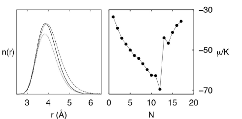
Figure 1: Left panel: radial density distribution function of $p$H₂ molecules in CO@($p$H₂)_n (dotted line: $n=11$, continuous line: $n=12$; dash-dotted line: $n=13$). Right panel: $p$H₂ chemical potential ($\mu_{N}=E_{n}-E_{n-1}$) as a function of the cluster size in CO@($p$H₂)_n.

In Fig. 1 we display the radial distribution functions of $p$H₂ around a CO molecule, for cluster sizes around the magic number $n=12$ botti . For $n\leq 12$ the magnitude of the maximum of these functions increases with the cluster size. For $n\geq 12$ this value stays nearly constant and the increase of the cluster size shows in the tail of the distribution, rather than in the height of the peak, indicating that the first solvation shell is completed at this magic number. For $n=12$ the absolute value of chemical potential also displays a maximum, suggesting the greatest stability of the clusters at this size. At the same time, the rotational distortion constant displays a minimum, indicating the largest rigidity of this clusters. All these findings suggest that the propensity of the $p$H₂ droplet to crystallize is maximum ad this cluster size. This fact has to be compared with the findings of Ref. ceperley_h2 which show clear signs of superfluidity in a cluster of 13 $p$H₂ molecules, whose structure is similar to that of CO@($p$H₂)_n with the solvated CO molecule substituted with a $p$H₂ molecule. In order to assess the melting vs. freezing behavior of finite systems, we introduce a dynamical criterion based on the persistence of geometrical signatures of the crystal structure.

The shape of a rigid body is well described by the multipole moments of, say, its mass density distribution around the center of mass, $Q^{l}_{m}$. In order to characterize the degree of rigidity of a cluster which, in addition to shape fluctuations, also experiences rotational diffusion, the shape must be described in a way which is independent of the orientation. The magnitude of the multipole, defined as $q^{l}=\sum_{m}{Q^{l}_{m}}^{*}Q^{l}_{m}$, provides such an invariant characterization of a rigid body. This quantity, however, is not suitable to discriminate the cases where a given multipole vanishes on the average, and $\langle q^{l}\rangle\neq 0$ because of the fluctuations, from those where a non vanishing value of $\langle q^{l}\rangle$ is due to the average shape of the cluster. This discrimination is best achieved in terms of a suitably defined rotationally-invariant time correlation functions of the various multipole moments in the rotating-axes frame. In order to proceed, let us define an effective angular velocity, $\mathbf{\Omega}(\tau)$, as the average of the forward angular velocities of the individual molecules. The operator corresponding to the global rotation accomplished in a time step $\epsilon$ reads:

$$\Delta R(\tau)={\rm e}^{-i\epsilon{\bf L}\cdot\mathbf{\Omega}(\tau)},$$ (10)

where $\bf L$ is the generator of the rotation group (angular momentum). The total rotation accomplished during a time $\tau$ is:

$$R(\tau) = {\cal T}{\rm e}^{-i\int_{0}^{\tau}{\bf L}\cdot\mathbf{\Omega}(\tau^{\prime})d\tau^{\prime}}$$ (11)

$$\equiv \prod_{n=1}^{T/\epsilon}\Delta R(n\epsilon),$$ (12)

where ${\cal T}{\rm e}^{(\cdot)}$ indicates the time-ordered exponential. With the aid $R(\tau)$ we define a rotating-axes multipole time-correlation function, $c_{l}(\tau)$, as the correlation between the multipole moment at (imaginary) time $\tau^{\prime}$ and the multipole at time $\tau^{\prime}+\tau$, rotated by $R(\tau^{\prime})^{-1}$ (time-translation invariance implies that these correlations are independent of $\tau^{\prime}$):

$$c_{l}(T)={\sum_{m}\left\langle Q^{l*}_{m}(\tau)\bar{Q}^{l}_{m}(\tau+T)\right\rangle\over\sum_{m}\left\langle Q^{l*}_{m}(\tau)Q^{l}_{m}(\tau)\right\rangle},$$ (13)

where $Q^{l}_{m}(\tau)$ is the multipole moment of the system at (imaginary) time $\tau$, the brackets, $\langle\cdot\rangle$, indicate an average over the random walk, and $\bar{Q}$ indicates the multipole rotated by $R^{-1}(\tau)$. If a system is rigid, $c_{l}(\tau)$ is independent of time, whereas it tends to zero at large values of $\tau$ whenever the shape of the system undergoes random fluctuations. A large value of $c_{l}(\tau)$ at large times is thus an indicator of the persistence of the shape of the system paolo .

In the case of CO@($p$H₂)₁₂ our simulations indicate a very rapid decay of the correlations for all the multipoles up to and including $l=5$. For $l=6$, instead, after a short transient in which a very steep drop occurs, the correlations decay very slowly, indicating a long persistence of a shape compatible with a nonvanishing $l=6$ multipole and vanishing multipoles with smaller values of $l$. In Fig. 2 we report the $l=6$ rotating-axes multipole time correlation function calculated for CO@($p$H₂)₁₂.

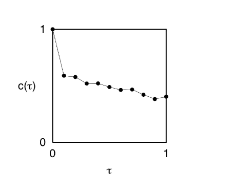
Figure 2: $l=6$ rotating-axes multipole time correlation function (Eq. 13) for CO@($p$H₂)₁₂.

This behavior is indeed compatible with a regular icosahedral shape, whose lowest non-vanishing multipoles correspond to $l=6$ and $l=10$. In order to visualize the intrinsic shape of the cluster, we calculate the rotating-axes number density distribution of the hydrogen molecule, $\bar{n}_{\rm H_{2}}({\bf r})$, by rotating each configuration of a quantum path at imaginary time $\tau$ with respect to the first configuration by $R^{-1}(\tau)$, as defined in Eqs. (12). The contribution to the density from each quantum path sampled by our RQMC procedure is then further rotated, so as to minimize the mutual distance of the particle centroids resulting from different paths. In Fig. 3 we display the rotating-axes number densiy distribution resulting from our simulations for CO@($p$H₂)₁₂.

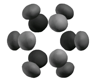
Figure 3: $p$H₂ rotating-axes number-density distribution for CO@($p$H₂)₁₂ (see text). The displayed iso-surface corresponds to a value of the density including 60% of the total number of H₂ molecules. The solvated CO molecule rotates nearly freely with respect to the rotating-axes frame, and it is not displayed in the figure.

The results displayed in Figs. 2 and 3 seem to indicate that CO@($p$H₂)₁₂ clusters behave much as rigid bodies, the closest realization of a crystal in a finite system. This behavior is different from that found in Ref. ceperley_h2 for undoped ($p$H₂)₁₃ clusters whose structure is expected to be very similar to that of CO@($p$H₂)₁₂, the main difference being the substitution of the central CO molecule with another $p$H₂ molecule. In that paper the behavior of ($p$H₂)₁₃ was described as that of a structured superfluid, possibly resembling a supersolid ceperley_h2 . The prediction of a liquid-like behavior for ($p$H₂)₁₃—as well as its enhanced stability with respect to small clusters of different size—is supported by recent Raman spectroscopy measurements of cryogenic ($p$H₂)_n free jets toennies-PRL . Diffusion quantum Monte Carlo simulations presented in that paper were used to assign individual vibrational lines to clusters of different size, and they support the delocalized character of these systems, as well as the greatest stability of ($p$H₂)₁₃.

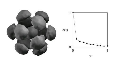
Figure 4: Left panel: $p$H₂ rotating-axes number density distribution for ($p$H₂)₁₃ (see text). The displayed iso-surface corresponds to a value of the density including 60% of the total number of $p$H₂ molecules. Right panel: $l=6$ rotating-axes multipole time correlation function (Eq. 13) for the same system.

In Fig. 4 we report the rotating-axes number-density distribution and the $l=6$ rotating-axes multipole time correlation function, resulting from RQMC simulations for ($p$H₂)₁₃. Although the number density distribution displays a nicely icosahedral shape—as it is the case for CO@($p$H₂)₁₂—the $l=6$ multipole correlation function displays a behavior which—as it will be shown below—is typical of a molten cluster. We interpret this seemingly contradictory behavior as a consequence of higher frequency of quantum inter-molecular exchanges in ($p$H₂)₁₃ than in CO@($p$H₂)₁₂. This is due to both the lack of exchanges between molecules in the outer shell and the central molecule in CO@($p$H₂)₁₂, and also to a larger binding of the molecules in the outer shell to the central one, which acts as to hinder intra-shell exchanges. During an exchange the shape of the cluster strongly departs from icosahedral. We expect therefore that—when the ratio between the typical duration of an exchange process and the waiting time between two exchanges increases—the $l=6$ multipole autocorrelations would decrease rapidly. It is interesting to notice that—contrary to CO@($p$H₂)₁₂, where the decay of the $l=6$ autocorrelations is much slower than for smaller angular momenta—in the case of ($p$H₂)₁₃ autocorrelations of different multipoles decay in a qualitatively similar way.

Figure 5: Left panel: $p$H₂ rotating-axes number density distribution for CO@($p$H₂)₁₃ (see text). The displayed iso-surface corresponds to a value of the density including 60% of the total number of $p$H₂ molecules. Right panel: $l=6$ rotating-axes multipole time correlation function (Eq. 13) for the same system.

In Fig. 5 we report the rotating-axes number density distribution and the $l=6$ rotating-axes multipole time correlation function, resulting from RQMC simulations for CO@(H₂)₁₃. The shape of the number-density iso-surface is strongly irregular, as a consequence of the quantum exchanges between one of the $p$H₂ molecules in the first solvation shell and the additional (thirteenth) molecule at the center of the cluster. The $l=6$ multipole time correlations correspondigly display a rather fast decay. The decay of the these correlations is in fact slower than for (H₂)₁₃ for which, however, the shape of the number-density isosurface is much more regular (only somewhat broadened with respect to CO@(H₂)₁₂ which we would qualify as a solid cluster).

Conclusions

We understand that our results—while confirming much of what is already known about the quantum behavior of $p$H₂ clusters ceperley_h2 ; toennies-PRL ; botti and their greater propensity to crystallize when they are seeded by a foreign molecule levi —probably raise more questions than they answer. A full understanding of the melting vs. freezing behavior in these exotic, yet very interesting, quantum systems will require much more work than it has been possible to report in this paper.

- (1) R. Car and M. Parrinello, Phys. Rev. Lett. 55, 2471 (1985).
- (2) S. Baroni, P. Giannozzi, and A. Testa, Phys. Rev. Lett. 58, 1861 (1987).
- (3) D. M. Ceperley, Rev. Mod. Phys. 67, 279 355 (1995) and references quoted therein.
- (4) See, e.g.: Monte Carlo method in the physical sciences, AIP Conference proceedings. Vol.690, edited by J.E. Gubernatis (Melville: American Institute of Physics).
- (5) W.M.C. Foulkes, L. Mitas, R.J. Needs, and G. Rajagopal, Rev. Mod. Phys. 73, 33 (2001).
- (6) S. Baroni and S. Moroni, Phys. Rev. Lett. 82, 4745 (1999), and in Quantum Monte Carlo Methods in Physics and Chemistry, edited by P. Nightingale and C.J. Umrigar. NATO ASI Series, Series C, Mathematical and Physical Sciences, Vol. 525, (Kluwer Academic Publishers, Boston, 1999), p. 313 (see also: http://xxx.lanl.gov/abs/cond-mat/9808213).
- (7) S. Moroni and S. Baroni, Proceedings of the Conference on Computational Physics 2004, edited by M. Ferrario, C. Pierleoni, and S. Melchionna, Comp. Phys. Comm. in press (2005).
- (8) V.L. Ginzburg and A.A. Sobyanon, JETP Lett. 15, 242 (1972).
- (9) P. Sindzingre, D.M. Ceperley, and M.L. Klein, Phys. Rev. Lett. 67, 1871 (1991).
- (10) S. Grebenev, B. Sartakov, J.P. Toennies, and A.F. Vilesov, Science 289, 1532 (2000).
- (11) A.C. Levi and R. Mazzarello, J. Low Temp. Phys. 122, 75 (2001); R. Mazzarello and A.C. Levi, J. Low Temp. Phys. 127, 259 (2002).
- (12) Y. Kwon and K.B. Whaley, Phys. Rev. Lett. 89, 273401 (2002).
- (13) G. Tejeda, J.M. Fernández, S. Montero, D. Blume, and J.P. Toennies, Phys. Rev. Lett. 92, 223401 (2004).
- (14) M.C. Gordillo and D.M. Ceperley, Phys. Rev. Lett. 79, 3010 (1997).
- (15) M. Boninsegni, Phys. Rev. B 70, 125405 (2004).
- (16) A. Sarsa, K.E. Schmidt and W.R. Magro, J. Chem. Phys. 113, 1366 (2000).
- (17) See the special topic issue on He nanodroplets, J. Chem. Phys. 115, 10065-10281 (2001).
- (18) S. Moroni, M. Botti, S. de Palo, and A.R.W McKellar, J. Chem. Phys. in press (2005).
- (19) After this paper was completed and submitted, we learnt from Paolo Giaquinta that ideas similar to ours had been developed by him long ago to study the local structure of classical fluids (P. Giaquinta, CECAM internal report (Paris, 1978), unpublished).