Frustrated Quantum Magnets

Abstract

A description of different phases of two dimensional magnetic insulators is given.

The first chapters are devoted to the understanding of the symmetry breaking mechanism in the semi-classical Néel phases. Order by disorder selection is illustrated. All these phases break $SU(2)$ symmetry and are gapless phases with $\Delta S_{z}=1$ magnon excitations.

Different gapful quantum phases exist in two dimensions: the Valence Bond Crystal phases (VBC) which have long range order in local S=0 objects (either dimers in the usual Valence Bond acception or quadrumers..), but also Resonating Valence Bond Spin Liquids (RVBSL), which have no long range order in any local order parameter and an absence of susceptibility to any local probe. VBC have gapful $\Delta S=0,or1$ excitations, RVBSL on the contrary have deconfined spin-1/2 excitations. Examples of these two kinds of quantum phases are given in chapters 4 and 5. A special class of magnets (on the kagome or pyrochlore lattices) has an infinite local degeneracy in the classical limit: they give birth in the quantum limit to different behaviors which are illustrated and questionned in the last lecture.

Chapter 1 Introduction

In this first chapter, we rapidly describe the basic knowledge on Heisenberg magnets to set the frame and the notations of the next developments. Different excellent text books can be used for a wider and slower introduction [1, 2, 3].

1.1 History

The first microscopic model for magnetism goes back to Heisenberg when he realized in 1928, that the exchange energy between electrons (introduced by Dirac and himself to explain the singlet triplet separation of the gaseous helium spectrum) was also responsible for ferromagnetism. Heisenberg and Dirac have first suggested that exchange of electrons could be written in an effective way in spin space through the use of a spin Hamiltonian, which reads:

$$h(i,j)={\bf{S}}_{i}.{\bf{S}}_{j}$$ (1.1)

where ${\bf{S}}_{i}$, ${\bf{S}}_{j}$ are the spin-1/2 operators of electrons i and j .

This Hamiltonian allows the basic description of the magnetism of insulators on a lattice (Heisenberg and Van Vleck). In its simplest form, it is written:

$${\cal H}=J\sum_{<i,j>}{\bf{S}}_{i}.{\bf{S}}_{j}$$ (1.3)

where the sum $<i,j>$ runs on pairs of next neighbor sites and $J$ measures the strength of the effective coupling ( related to the tunnel frequency of a pair of electrons on two neighboring sites).

The Heisenberg Hamiltonian, as the more complex schemes of interactions that will be studied in these lectures, are all $SU(2)$ invariant (i.e. invariant in a global spin rotation). On a given sample of $N$ spins, ${\cal H}$ commutes with the total spin of the sample $S_{tot}$:

$$\left[{\cal H},S^{2}_{tot}\right]=\left[{\cal H},S^{z}_{tot}\right]=0.$$ (1.4)

The eigen-states of ${\cal H}$ can thus be characterized by their total energy and their total spin $S_{tot}$. Eigen-states of ${\cal H}$ with different $S_{tot}$ are a priori non degenerate.

1.2 $J<0$: the ferromagnet

If $J$ is $<0$, the ground-state of (1.3) can be readily written as:

$$|F_{z}>=\prod_{i}|i,\,+>$$ (1.5)

where the ket $|i,\,+>$ indicates that spin at site i is in the eigen-state of $S^{z}_{i}$, with eigen-value $+\hbar/2$ (in the following we will use $\hbar=1$) and the tensorial product involves each lattice spin.

It is easy to show that this state (1.5) is an eigen-state of (1.3) with the total energy:

$$E_{ferro}=N\frac{z}{2}\;\frac{J}{4},$$ (1.6)

where $N$ is the number of spins of the sample, and $z$ the coordination number of the lattice. It is also an eigen-state of the total spin $S^{2}_{tot}$ and its $z$-component $S^{z}_{tot}$with eigen-values $N/2(N/2+1)$ and $M^{z}_{tot}=N/2$. It minimizes the energy of each bond and is thus the ground-state of (1.3). This state can be written without ambiguity as:

$$|F_{z}>=|S_{tot}=N/2,\,M^{z}_{tot}=N/2>$$ (1.7)

It is degenerate with the $2N$ other eigen-values of $S^{z}_{tot}$, running from $N/2-1$ to $-N/2$.

You should notice that in the thermodynamic limit such a degeneracy is negligible: the associate entropy of the extensive ground-state is ${\cal O}(Ln(N))$, which does not contradict Nernst Theorem.

On a macroscopic sample, $|F_{z}>$ describes a system with a macroscopic magnetization pointing in the $z$ direction. Using the total spin operator this state could be rotated in any direction $\bf u$ defined by the Euler angles $(\theta,\phi)$ with respect to the reference frame . We thus obtain the quantum description of a coherent state with a magnetization in the $\bf u$ direction:

$$|F_{{\bf u}}>=e^{iS^{z}_{tot}\phi}e^{iS^{y}_{tot}\theta}|F_{z}>.$$ (1.8)

Let me underline that this coherent state remains in the ferromagnetic ground-state multiplicity and that its total spin is well defined and equal to $N/2$.

The semi-classical character of such states is embodied in the following property: the quantum overlap of two states pointing in different directions decreases exponentially with $S_{tot}$, that is with the system size $N$ [3]. For macroscopic samples, the state of a ferromagnet can thus be described with classical words and concepts. This can be said in another way: the macroscopic spin, understood as a quantum observable, obeys quantum commutation relationships:

$$[S^{x}_{tot},S^{y}_{tot}]=iS^{z}_{tot}$$ (1.9)

as $S_{tot}$ is proportional to $N$, the relative value of the “quantum fluctuations” (measured by the commutator/$N^{2}$) becomes negligible in the thermodynamic limit.

The selection of a special state as (1.5) to describe the ferromagnetic ground-state is a “minor (or trivial?) symmetry breaking” of the problem. By $SU(2)$ rotations this eigen-state generates all the ground-state multiplicity, and this multiplicity only .

1.3 $J>0$: Néel antiferromagnet and spin gapped Phases

1.3.1 A few historical markers

If J is $>0$ the ground-state of (1.3) is absolutely not obvious. In 1932, Néel suggested that the description of experiments was consistent with a picture of the ground-state as a special arrangement of ferromagnetic sublattices with a zero total magnetization.

Let us examine the simplest case of the Heisenberg problem on the square lattice. This lattice may be partitioned in two sublattices A and B with a double unit cell. Each spin of the A (resp. B) lattice is exclusively coupled to the B (resp. A) lattice . Such a problem is said bipartite . In this case we usually write Néel’s wave-function as:

$$|Cl.\;N\acute{e}el\;w.f.>=\prod_{i\in A,\,j\in B}|i\;,\;+>\,|j\;,\;->$$ (1.10)

This state has indeed a zero component of the total spin in the $z$ direction, but it is non zero in the $xy$ plane. This Ising state has maximal sublattice magnetizations: $S_{A,B}=\frac{N}{4},\;M_{A,B}=\pm\frac{N}{4}$. The Ising state with a zero component of the total spin in the ${\bf u}$ direction, defined by the Euler angles $\theta$ and $\phi$, is indeed:

$$|Cl.\;N\acute{e}el\;w.f.;{\bf u}>=e^{iS^{z}_{tot}\phi}e^{iS^{y}_{tot}\theta}|Cl.\;N\acute{e}el\;w.f.>$$ (1.11)

In this antiferromagnetic case the idea that it is possible to restore the overall symmetry of the problem by rotation of (1.10) and averaging has more far fetching consequences that is usually thought!

In his biography Néel told that he had to face strong skepticism and objections specially from C.J. Görter (colloquium in Leyden at the Kammerlingh Onnes Lab; 1932). It seems that L. Landau equally rapidly discarded this special variational wave-function with the same objections as C. J. Görter.

I have not had access to authenticated sources, but the objections were probably of two kinds:

• The Néel state strongly breaks the $SU(2)$ symmetry of the Hamiltonian and cannot be a good candidate to describe an eigen-state,

• The existence of ferromagnetic sublattices is not proved and elementary quantum mechanics seems in strong disagreement with this assumption.

1.3.2 $SU(2)$ symmetry breaking of the Néel states.

As I will explicit below and explain in details in the next chapter, the Néel states breaks the $SU(2)$ symmetry of the Heisenberg Hamiltonian (and the lattice geometrical symmetries) in a radical way (quite different from the ferromagnetic case).

The classical Néel state is not an eigen-state of the total spin, and as such it can only be described as a linear combination of many eigenstates of (1.3).

In order to have an elementary view of this question let us rephrase Néel wave-function in simple quantum terms: two ferromagnetic sublattices A and B, defined by their total spins $S_{A,B}=N/4$ are to be coupled in such a way that:

$$(S^{z}_{A}+S^{z}_{B})|Cl.\;N\acute{e}el\;w.f.>=0$$ (1.12)

We know from elementary spin algebra that there are $(N/2+1)$ $SU(2)$ invariant ways to do this: the different states resulting of this coupling can be labeled in an unique way by their total spin $S_{tot}$, which can range (for even N) from $S_{tot}=0$ to $S_{tot}=N/2$. They can be written in an unambiguous way under the form $|\frac{N}{4},\frac{N}{4},S_{tot},M_{S}>$. In any of these subspaces, one can indeed select the $M_{S}=0$ component of the total spin, thus fulfilling Néel prescription.

Elementary spin algebra leads to the following expression for the classical Néel state wave-function:

$$|Cl.\;N\acute{e}el\;w.f.>=\sum_{S,M_{S}}{\frac{(-1)^{M_{S}}}{\sqrt{2S+1}}}\left(\begin{array}[]{ccc}N/4&N/4&S\\ N/4&-N/4&M_{S}\\ \end{array}\right)|S_{A},S_{B},S,M_{S}>$$ (1.13)

where $S$ runs through the $N/2+1$ possible values of $S_{tot}$, and in general for each value of $S$, $M_{S}$ runs from $-S$ to $+S$. Here the selection rule on the $z$ components of the spins implies that $M_{S}=0$. In this expression the coefficients $\left(\begin{array}[]{ccc}S_{A}&S_{B}&S\\ M_{A}&M_{B}&M_{S}\\ \end{array}\right)$ are known as Wigner “3j” symbols. These coefficients are the coefficients of the unitary transformation which transforms the uncoupled sublattice spins $S_{A,B}$ to the $SU(2)$ invariant coupled combinations. The Wigner “3j” symbols can be calculated by elementary algebra, they are tabulated in books and in computer libraries.

Comparison of this antiferromagnetic coherent state (1.13) to the ferromagnetic one (1.5), (1.7) shows explicit qualitative differences: the ferromagnetic state is a state with a definite total spin $N/2$, whereas (1.13) involves components with total spin ranging from $0$ to $N/2$. This shows that Néel wave-function can at best be described as a linear combination of a large number of eigen-states of ${\cal H}$.

For bipartite lattices a theorem originally due to Hulthen (1938)[4], Marshall (1955)[5] and strengthened by Lieb and Mattis (1962)[6] states that the absolute ground-state of the antiferromagnetic Heisenberg (1.3) (and of more general antiferromagnetic models respecting the bipartition of the lattice) is unique and has total spin zero. Moreover the ground-state energies in each $S$ sector are ordered accordingly to $S_{tot}$:

$$\forall S^{{}^{\prime}}_{tot}>S_{tot}\hskip 28.45274ptE_{0}(S^{{}^{\prime}}_{tot})>E_{0}(S_{tot}).$$ (1.14)

From that point, we might infer that the $|S_{A}=N/4,S_{B}=N/4,0,0>$ state would be a good starting point to describe the absolute ground-state $|\Psi_{0}>$ of (1.3), and forget all the other components of the classical Néel state (1.13). But in such a point of view, we lose the foundations for the semi-classical approaches: a state with total spin 0 does not allow to point any direction in spin space. According to Wigner Eckart theorem, the three components of the sublattice magnetizations (as the components of any vector) are simultaneously and exactly zero in such a state:

$$<{\Psi}_{0}|{\bf S}_{A,B}|\Psi_{0}>\;\;\;\propto\;\;\;<\Psi_{0}|{\bf S}_{tot}|\Psi_{0}>\;\;\;=\;\;0.$$ (1.15)

To answer Görter and Landau objection, and support Néel picture for quantum antiferromagnets, it is thus necessary to show that eigen-states with different $S_{tot}$ appear in the exact spectrum as the different $SU(2)$ invariant components of the supposed-to-be quantum Néel state and are degenerate in the thermodynamic limit. In such a limit, a quantum superposition of these eigen-states embodies the “strong” symmetry breaking associated to Néel’s scenario. Such a mechanism has been described in full length by P. W. Anderson in two books [7, 8, 9].

In this chapter and for the sake of simplicity only bipartite lattices and collinear Néel states are studied.

1.3.3 Ferromagnetic sublattices, “quantum fluctuations” and dimer pairing

The second difficulty with Néel’s scenario, the existence of ferromagnetic sublattices cannot be supported by quantum mechanics without specific calculations. In fact the sublattice magnetizations are not good quantum numbers, they are decreased and eventually wiped out by ”quantum fluctuations”. This point is common knowledge today. An essential stone mark to this understanding is the first spin-wave calculations done in 1952 by P.W.A. Anderson [7] and R. Kubo [13] .

In this approach one clearly sees that the transverse term of the Heisenberg Hamiltonian:

$${\bf{S}}_{i}.{\bf{S}}_{j}|i,+>|j,-> = {S}^{z}_{i}\,{S}^{z}_{j}\;\;|i,+>|j,->\;+$$ (1.16)

$$+\;1/2\;\left[{S}^{+}_{i}\,{S}^{-}_{j}+{S}^{-}_{i}\,{S}^{+}_{j}\right]\;|i,+>|j,->$$

$$= -\frac{1}{4}\;\;|i,+>|j,->+\frac{1}{2}\;\;|i,->|j,+>$$

induces spin-flips, decreasing the sublattice magnetizations. These low energy excitations (spin-waves) can be described as quantum oscillators: they have zero point quantum fluctuations, which renormalize and stabilize the Ising energy and decrease the sublattice magnetization. This spin-wave calculation lays on an $\frac{1}{S}$ expansion and its validity for spins$-1/2$ has often be questioned. It appears to be qualitatively valid when compared to exact results (when they exist) or to more sophisticated numerical work (see Table 1), I will explain in the next chapter the physical reason of this ”good” behavior.

To my knowledge exact results exist for 1-dimensional systems (Bethe problem, Majumdar -Gosh $J_{1}-J_{2}$ problem) where they predict the absence of Néel long range order (and algebraic spin-spin decaying correlations in the first case, exponentially decaying ones in the second case). For larger lattice dimensionality, only the case of the cubic lattice has been shown to be Néel ordered [14]. On the other hand, the Mermin-Wagner theorem precludes existence of Néel long range order (NLRO) at $T\neq 0$ for lattices with dimension $d<3$. This theorem does not give any indications for the $T=0$ behavior of 2-dimensional magnets which are the central point of these lectures. (Rigorous proofs of order exist for spin 1 and larger [15, 16, 17].)

Néel order versus dimer pairing: naive approach and numerical results.

The classical Néel wave-function (1.10), is a variational solution with an energy per bond $(-\frac{J}{4})$. Whereas the quantum ground-state of (1.1) is:

$$|(i,j)>=\frac{1}{\sqrt{2}}\left[|i,+>|j,->-|i,->|j,+>\right]$$ (1.17)

with the energy $-\frac{3}{4}J$. This state that we will call either a singlet state or a dimer realizes a very important stabilization of a pair of spins (if compared to the classical state) but it does not allow to point any direction in spin space (it is a state with a total spin zero). At this microscopic scale quantum mechanics in its radicalism does not favor the idea of an $SU(2)$ symmetry breaking. The controversy on the existence of Néel long range order, specifically in frustrated ($\equiv$ triangular) geometry or with competing interactions has been a long lasting debate opened by P.W.A. Anderson and P. Fazekas [18, 19] and fueled again in 1987 with the discovery of High Temperature Superconductors in cuprates.

When looking in a simple-minded way at a lattice of coordination number $z$, the energy balance between the classical Ising-like Néel state and the quantum dimer covering is not so clear. The classical Néel state has an energy

$$E_{cl}=\frac{N}{2}z\frac{J}{4}cos(\theta)$$ (1.18)

(where $\theta$ is the angle between sublattice magnetizations) to be compared to the quantum energy of a dimer covering

$$E_{dim}=-\frac{N}{2}3\frac{J}{4}.$$ (1.19)

This simple approach predicts Néel order on the square lattice, it is inconclusive for the hexagonal lattice, or the triangular lattice (which have Néel long range order) and it predicts that the Heisenberg model on the kagome lattice is disordered (which is correct, see Table 1.1).

	Coordination	$2<{\bf S}_{i}.{\bf S}_{j}>$
Lattices	number	per bond	$M/M_{cl}$
dimer	1	-1.5
1 square	2	-1
1 D Chain	2	-0.886	0
honeycomb [20]	3	-0.726	0.44	bipartite
sq-hex-dod. [21]	3	-0.721	0.63	lattices
square [22]	4	-0.669	0.60
classical value		-0.5	1
one triangle	2	-0.5
kagome [23]	4	-0.437	0	frustrating
triangular [11]	6	-0.363	.50	lattices
classical value		-0.25	1
1 tetrahedron	3	-0.5
checker-board [fmsl03]	6	-0.343	0	frustr. latt.

Table 1.1: Quantum energy per bond and sublattice magnetization in the ground-state of the spin-1/2 Heisenberg Hamiltonian on various simple cells and lattices. The sq-hex-dod. is a bipartite lattice formed with squares, hexagons and dodecagons.

Indeed this approach is naive in both limits.

In the classical limit we have neglected the ”fluctuation effects” generated by the transverse coupling: these fluctuations effectively contribute noticeably to the stabilization of the ground-state of ordered systems (see Table 1.1).

In the quantum disordered limit, the dimer covering solutions do not take into account the resonances between different non orthogonal coverings which are very numerous and are an essential concept for understanding the Resonating Valence Bond Spin Liquids (concept introduced in the present context by P. W. Anderson in 1973 and named in honor to Linus Pauling). The existence of this second kind of phases remained speculative until the end of the nineties. We now think that these different scenarios can be realized in two dimensional spin-1/2 quantum antiferromagnets (see Table 1.2).

Phases	G.-S. Symmetry Breaking	Order Parameter
	SU(2)
Semi-class. Néel order	Space Group	Staggered Magnet.
	Time Reversal
		dimer-dimer LRO or
Valence Bond Crystal	Space Group	S=0 plaquettes LRO
R.V.B. Spin Liquid		No local
(Type I)	topological degeneracy	order parameter
R.V.B. Spin Liquid		No local
(Type II)	topological degeneracy	order parameter

Table 1.2: The four 2-dimensional phases described in these lectures.

In the first part of these lectures, I will try to extract the generic features of the Quantum Néel phase in a fully quantum $SU(2)$ invariant framework. In so doing I hope to be able to convince you that the symmetry breaking mechanism implemented in the Néel state could be understood from a completely quantum and rather simple approach.

In the second part of the lectures we will discuss the new quantum phases where the ground-state does not break $SU(2)$ symmetry and has no long range order in spin-spin correlations. We will see that at least two or three different phases with these general properties have been exhibited in realistic spin models. The differences between these quantum phases depend on the pattern of dimer-dimer correlations: either they display long range order and the system is a Valence Bond Crystal or any correlation functions are short ranged and it is a liquid (Resonating Valence Bond Liquid). We will try to describe the generic properties of their excitations, discuss some experimental prescriptions and recent results.

1.4 Miscellaneous remarks on the use of the words “quantum fluctuations”, “quantum disorder”

In antiferromagnets the word ”quantum fluctuations” is often used with different acceptions, depending on the context.

When we say in the spin-wave approach of the antiferromagnet that the sublattice magnetization can be wiped out by “quantum fluctuations” let be conscious that it is a model dependent concept! In that case these “quantum fluctuations” do not describe a real microscopic, time-dependent mechanism: it is just a way to describe a renormalization (we might say a dressing) of the Ising-like states.

On the other hand, when we say in the RVB spin liquid state, that the system can fluctuate between different dimer covering configurations this correspond to true excitations of the system which may be gapped or not.

Third, when neutronists say that they measured longitudinal or transverse spin fluctuations, they use the word in its strictest acceptance! The root mean square fluctuations of the sublattice magnetization is defined as $\sqrt{<\Psi_{0}|S^{2}_{A}|\Psi_{0}>}$ . It has the value $\sqrt{\frac{N}{4}(\frac{N}{4}+1)}$, in the classical Ising-like Néel state (1.13), and is still of order ${\cal O}(N)$ in any quantum ground-state with long range Néel order (as for example, on the square, hexagonal or triangular lattice). The same is true of the total spin fluctuations as we will understand in the next chapter! And this is observable! The staggered susceptibility is the experimental quantity that can be measured experimentally: it is related to the Fourier transform of the above correlation function. It is non zero in NLRO systems and zero in spin gapped ones.

In fact the fluctuations of the total spin are zero in a ”quantum disordered” system with a spin gap. But local fluctuations of a configuration of spins and dimers in a “quantum disordered” spin liquid can also be observed with local probes: as for example muons [25]….

Only a few examples of situations that can be uncovered by the loose expression “quantum fluctuations”!

Chapter 2 The semi-classical Néel phase: quantum mechanics and symmetry breakings

In this chapter we want to uncover in a very simple quantum mechanical point of view, the nature of the semi-classical phase and the ingredients of the $SU(2)$ symmetry breaking. This is grounded in the existence of a “tower” of $SU(2)$ invariant states which collapse in the thermodynamic limit in a ground-state multiplicity that can be described either in the $SU(2)$ invariant basis, or in an (overcomplete) basis of semi-classical coherent Néel states. We will do it first in a pedestrian calculus approach and then phrase is again in a more basic and conceptual point of view parallelizing the translational symmetry breaking of solids. The space symmetry breaking will be quickly discussed in this chapter. A more detailed study will be done in the next chapter where we analyze the mechanism of “order by disorder” in these semi-classical antiferromagnets.

2.1 Calculus approach

Let us consider the Heisenberg problem on a lattice of $N$ sites with periodic boundary conditions. It is interesting to look first to an exactly solvable model, that emerges easily from the expression of the Heisenberg Hamiltonian ( Eq. 1.3) in reciprocal space:

$${\cal H}=2J\sum_{k\,\in BZ}\gamma_{k}{\bf S_{k}.S_{-k}}.$$ (2.1)

In this expression:

$${\bf{S}_{k}}=\frac{1}{\sqrt{N}}\sum_{i}{\bf{S}_{i}}\;exp(-i{\bf k}.{\bf R}_{i})$$ (2.2)

where ${\bf R}_{i}$ is the coordinate of spin i, $N$ the (even) number of lattice sites and ${\bf k}$ runs on the reciprocal points of the lattice in the first Brillouin zone (BZ). $\gamma_{k}$ is the structure factor of the lattice:

$$\gamma_{k}=\frac{1}{2}\sum_{i=1,2}cos({\bf k}.{\bf e}_{i})$$ (2.3)

with ${\bf e}_{j},\,(j=1,2)$, the unit vectors generating the lattice. On this lattice the Néel state is invariant by 2-step translations associated to wave-vectors ${\bf k}=(0,0)$ and $\bf k={\bf k}_{0}=(\pi,\pi)$. Let us select these special components in the Heisenberg Hamiltonian and rewrite it as:

$${\cal H}={\cal H}_{0}+{\cal V}$$ (2.4)

with

$${\cal H}_{0}=2J({\bf S}_{0}^{2}-{\bf S}_{{\bf k}_{0}}.{\bf S}_{-{\bf k}_{0}})$$ (2.5)

$${\cal V}=2J\sum_{{\bf k}\in BZ^{*}}\gamma_{k}{\bf S}_{k}.{\bf S}_{-k}$$ (2.6)

where $BZ^{*}$ is to be understood as the first Brillouin zone minus the $\bf k=0$ and ${\bf k}_{0}$ points.

Simple algebra leads to:

$${\cal H}_{0} = 2J({\bf S}_{0}^{2}-{\bf S}_{{\bf k}_{0}}.{\bf S}_{-{\bf k}_{0}})$$ (2.7)

$$= \frac{4J}{N}({\bf S}_{tot}^{2}-{\bf S}_{A}^{2}-{\bf S}_{B}^{2}),$$

where ${\bf S}_{tot}$ is the total spin of the sample and ${\bf S}_{A,B}$ the total spins of the $A,\;B$ sublattices.

You might recognize in ${\cal H}_{0}$ the toy model used by Lieb and Mattis in the demonstration of the ordering theorem [6]: it describes a problem with constant long range interactions between spins on different sublattices and no interactions between spins on the same sublattice. This model can be solved exactly.

2.1.1 The Ising-like Néel state in an $SU(2)$ invariant model

Hamiltonian ${\cal H}_{0}$ (Eq. 2.7) is an $SU(2)$ invariant Hamiltonian which commutes with ${\bf S}^{2}_{tot}$ and ${\bf S}^{z}_{tot}$. It also commutes with ${\bf S}^{2}_{A,B}$, which in this model are conservative quantities (good quantum numbers). All these observables commute two by two and with ${\cal H}_{0}$ . Eigen-states of ${\bf S}^{2}_{tot}$, ${\bf S}^{z}_{tot}$, ${\bf S}^{2}_{A}$, ${\bf S}^{2}_{B}$ are also eigen-states of (2.7), with eigen-values:

$$E(S,S_{A},S_{B})=\frac{4J}{N}\left[S(S+1)-S_{A}(S_{A}+1)-S_{B}(S_{B}+1)\right]$$ (2.9)

The quantum numbers for a sample with an (even) number $N$ of sites are:

• $S_{A},S_{B}\in[0,1,..,N/4]$,

• For a given set of values of the sublattice magnetizations $(S_{A},S_{B})\;$ the value of the total spin $S\in[|S_{A}-S_{B}|,...,S_{A}+S_{B}]$,

• For a given value $S$ of the total spin of the sample, its $z$ component $M_{S}\;\in[-S,-S+1,....,S-1,S]$.

The ground-state in each $S$ sector $E_{0}(S)$ is obtained for the maximum sublattice magnetization $N/4$. The energies of these low energy states obey the following relation:

$$E_{0}(S)=-\frac{J}{2}(N+4)+\frac{4J}{N}\left[S(S+1)\right]$$ (2.10)

.

The eigen-states associated to these eigen-values are the $SU(2)$ invariant components of the Ising-like Néel state $|S_{A}=N/4,S_{B}=N/4,S\,,M_{S}>$ introduced in section 1.3.2 (Eq. 1.13). These eigen-states have four essential properties:

• their number and their spatial symmetries are uniquely defined by the coupling of the sublattice magnetizations (these are exact necessary requirements),

• their sublattice magnetization is N/4,

• they collapse to the absolute ground-state as ${\cal O}(\frac{1}{N})$.

These levels form a set that has been described by Anderson as a “tower” of states [7, 8, 9]: we have called them in our original paper QDJS (for quasi degenerate joint states). In this lectures we will refer to this set as the Anderson tower.

On a finite size lattice the classical Néel state (1.13) is a non stationary state of ${\cal H}_{0}$ (eq. 2.7). But, its precession rate decreases as ${\cal O}(\frac{1}{N})$ with the system size and becomes infinitely slow in the thermodynamic limit.

The coherent Néel states described by Eq.(1.11), form an (overcomplete) basis of this ground-state multiplicity. The present study of their $SU(2)$ invariant representation shows that the multiplicity of this subspace is ${\cal O}(N^{\alpha})$ where $\alpha$ is the number of sublattices of the classical Néel state[11, 12]. This gives a non extensive entropy of the ground-state at $T=0$ in agreement with Nernst theorem.

Excitations

In this model an excited state is obtained by flipping a single spin of a sublattice. From equation (2.9) one sees that these excitations are localized and have an energy:

$$E^{exc}_{Ising}=2J\left[1+\frac{4(S+1)}{N}\right].$$ (2.11)

For any size these excitations are gapful and ${\cal O}(J)$.

Conclusion

${\cal H}_{0}$ describes an Ising magnet in an $SU(2)$ invariant framework: its spectrum has the very simple structure schematized in Fig. 2.1.

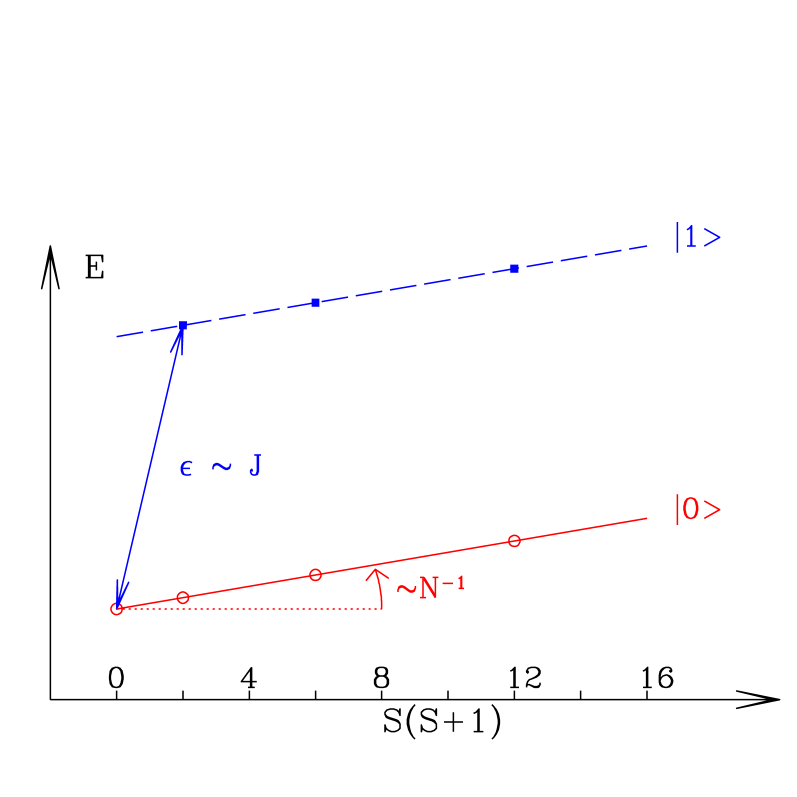
Figure 2.1: Typical spectrum of a finite size collinear Ising magnet. The tower of eigen-levels joined by the continuous line and noted $\left|0\right>$ is the Anderson tower of states needed to form a symmetry breaking Ising ordered ground-state (Eq. 2.13): such a state is non stationary on a finite size sample. The second set $\left|1\right>$ (dashed line) is associated with the lowest excitations, which are highly degenerate and non dispersive.

In the thermodynamic limit this magnet can be described either in an $SU(2)$ invariant language with the help of the $|S_{A},S_{B},S,M_{S}>$ states or with the coherent semi-classical Néel states described in Eq.(1.11). The two basis are connected by exact transformation laws, Eq.(1.13) and its inverse:

$$|N/4,N/4,S,M_{S}>=(2S+1)\int d\tau D^{\dagger}_{s}(\phi,\theta)|Cl.\;N\acute{e}el\;w.f.;{\bf u}>,$$ (2.12)

where the differential integration volume reads $d\tau=\frac{1}{4\pi}d\phi d(cos\theta)$, where $\phi\in[0,2\pi]$, $\theta\in[0,\pi]$ and $D_{S}$ is the rotation matrix in the $S$ subspace. In the thermodynamic limit, the symmetry breaking point of view is as valid as the $SU(2)$ invariant approach.

2.1.2 “Quantum fluctuations” in the Heisenberg model

Modification of this picture in an Heisenberg magnet with next neighbor exchange comes from the effect of the perturbation term ${\cal V}$ described in Eq. (2.6). ${\cal V}$ does not commute with ${\bf S}_{A}^{2}$ and ${\bf S}_{B}^{2}$: at first order in perturbation each component of ${\cal V}$ couples the ground-state of ${\cal H}_{0}$ in each $S$ sector (which are characterized by maximum uniform sublattice magnetizations) to states where the sublattice magnetization is decreased by one unit in some modulated way. The analytical treatment of this perturbation is uneasy in the $SU(2)$ invariant formalism, but indeed we recognize all the concepts at the basis of the usual algebraic spin wave approach: that is renormalization of the ground-state energy and of the sublattice magnetization by the zero point quantum fluctuations of the spin waves excitations.

If the structure of the tower of states i.e.:

• number and spatial symmetries of the states in each $S$ sector,

• existence in each of these states of a macroscopic sublattice magnetization (i.e. $\sqrt{<|S^{2}_{A}|>}\propto{\cal O}(N)$),

• scaling as ${\cal O}(\frac{JS(S+1)}{N})$ with respect to the ground-state,

resists to this renormalization, the nature of the ground-state multiplicity in the thermodynamic limit gives a new foundation to the spin-wave symmetry breaking point of view . The quantum Néel wave function thus emerges from the classical picture (Eq. 1.13) by the renormalization of the eigenstates $|S_{A},S_{B},S,M_{S}>$ of ${\cal H}_{0}$ under the action of ${\cal V}$. We can then write the quantum Néel wave-function as:

$$|Qu.\;N\acute{e}el\;w.f.>=\sum_{S,M_{S}}{\frac{(-1)^{M_{S}}}{\sqrt{2S+1}}}\left(\begin{array}[]{ccc}S_{A}&S_{B}&S\\ S_{A}&-S_{B}&M_{S}\\ \end{array}\right)\widetilde{|S,M_{S}>}_{0}$$ (2.13)

where the kets $\widetilde{|S,M_{S}>}_{0}$ are now the exact low lying states of the Anderson tower of ${\cal H}$ (Eq. 1.3).

2.1.3 The spin-wave algebraic approach

In order to gather all the material needed for a full understanding of the symmetry breaking mechanism in Néel antiferromagnets, let us recall the main results of a spin-wave calculation. (For the derivation of the spin-wave approach in antiferromagnets, see the above mentioned text-books [1, 2, 3].)

Departing from the Ising configuration (Eq.1.10), the transverse terms of the Heisenberg Hamiltonian create $\Delta S^{z}=1$ spin flips, which are mobile excitations.

• In an harmonic approximation these excitations are simply described as spin-waves, with frequencies:

  $$\omega_{\bf q}=2J\sqrt{1-\gamma^{2}_{\bf q}}$$ (2.14)

  where $\gamma_{\bf q}$ is the structure factor of the lattice defined in Eq.(2.3). The spin flips excitations are then dispersive, their frequency goes to zero when going to the two soft points ${\bf k=0,\;k_{0}}$. Around these points the dispersion law is linear in ${\bf k}$ (resp. $({\bf k-k_{0}})$).

• The zero point energy of these excitations (which are oscillator- like) renormalizes the Ising classical energy of the ground-state (1.18). To first order, this spin wave calculation gives the ground-state energy of the Heisenberg Hamiltonian on the square lattice as:

  $$E^{s-w}=-\frac{N}{2}z\frac{J}{4}-NJ+\sum_{{\bf q}\in BZ^{*}}\frac{\omega_{\bf q}}{2}$$ (2.15)

• These “ quantum fluctuations” also renormalize the sublattice magnetization. Let us define the order parameter $m$ in the ground-state $|0>$ of this symmetry breaking representation by:

  $$m=\frac{2}{NS}<0|S^{z}_{A}|0>.$$ (2.16)

  The first order spin-wave calculation leads to:

  $$m^{s-w}=1-{\frac{1}{N}}\sum_{{\bf q}\in BZ^{*}}\left[{\frac{1}{\omega_{\bf q}}}-1\right]$$ (2.17)

  The renormalization of the order parameter is dominated by the fluctuations in the low energy modes. The linear asymptotic behavior of $\omega_{\bf q}$ around the soft points, implies that the spin-waves correction to the order parameter diverges in 1D. It gives finite corrections at $T=0$ on most of the 2-dimensional lattices (square, triangular, hexagonal.. ).

• Finite Size Effects: The spin-wave approach allows a direct understanding of the finite size effects in a problem with Néel long range order. Let us first remind that on a finite size lattice of linear length $L$, the allowed wave vectors are quantized and of the form $\frac{2\pi}{L}$. This introduces a cut-off of the long wave-length fluctuations which is progressively relaxed as the size of the sample goes to $\infty$. As $\omega_{\bf q}$ is linear in ${\bf q}$ around the soft points, we thus expect that the ground-state energy $E^{s-w}$ (Eq. 2.15) and the order parameter $m^{s-w}$ (Eq. 2.17) on a lattice of finite size $L$ will differ from the $L\to\infty$ limits by factors of order ${\cal O}(\frac{1}{L})$. This is exactly the result obtained in more sophisticated approaches [26, 27, 28, 29, 30, 31].

  As we have already underlined the excitations of this model now differ from those of ${\cal H}_{0}$: they are itinerant and have acquired dispersion. On a finite lattice the energy needed to create the softest excitation is no more of order $J$, but of order $\frac{J}{L}\propto\frac{J}{N^{1/d}}$.

2.1.4 Self-consistency of the Néel picture for an Heisenberg magnet in an $SU(2)$ invariant picture: spectrum and finite size effects.

If the structure of the tower of states is essentially preserved by the quantum fluctuations due to ${\cal V}$, the semi-classical picture of coherent states is preserved (see subsection • ‣ 2.1.2), the spin-wave approach is a reasonable one and the essential results of this approach should appear in the full spectra of Eq.(1.3). Beyond the criteria already described to support the $SU(2)$ symmetry breaking, the following size effects should be present:

• The energy per site of the states of the low lying Anderson tower should converge to the thermodynamic limit with a leading correction term going as $\frac{1}{N\,L}\propto\frac{1}{L^{d+1}}$,

• The sublattice magnetization $\sqrt{<|S^{2}_{A}|>}$ in each of these states should remain ${\cal O}(N)$, with a leading term to the finite size corrections of order ${\cal O}\frac{1}{L}$,

• The low lying softest excitations with wave-vector $\frac{2\pi}{L}$ should be described by a second tower of states issued from the tower of excited states of the Ising model with one spin-flip (Eq. 2.11). But contrary to the Ising model, these states are now dispersive and the lowest excitation is now distant from the ground-state tower of states by an energy of the order of $\frac{J}{L}$: it is the Goldstone mode of the broken $SU(2)$ symmetry.

Some of these properties are summarized in the supposed-to-be spectrum of a Néel antiferromagnet described in Fig. 2.2 .

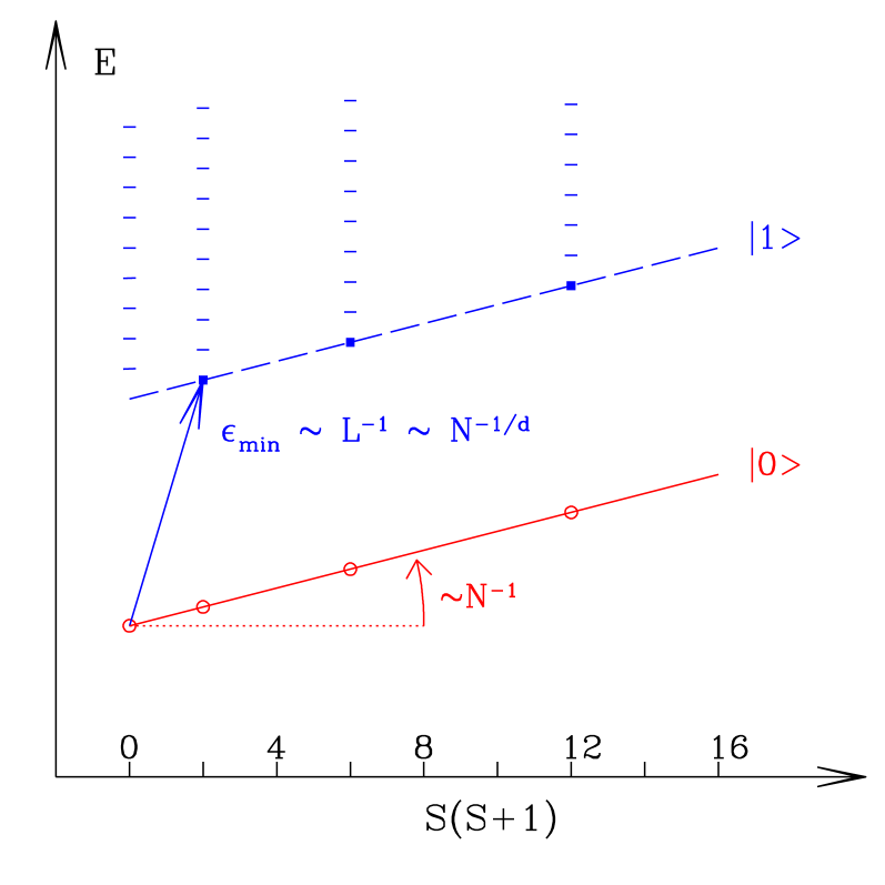
Figure 2.2: Typical spectrum of a finite size collinear antiferromagnet with Néel order. The tower of eigen-levels joined by the continuous line and noted $\left|0\right>$ is the Anderson tower of states needed to form a symmetry breaking Néel ordered ground-state (Eq. 2.13): such a state is non stationary on a finite size sample. The second set $\left|1\right>$ (dashed line) is associated with the lowest magnon.

This is to be compared to an exact spectrum of the Heisenberg Hamiltonian on a square lattice (Fig. 2.3)[32] or on an hexagonal lattice (Figs. 2.4, 2.6, 2.6 )[20].

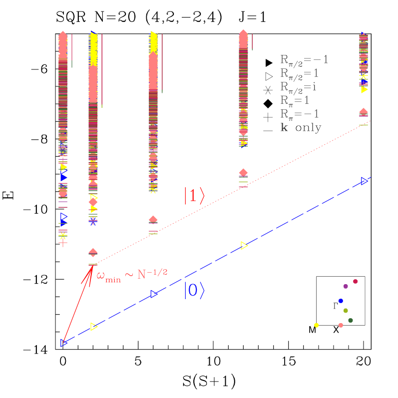
Figure 2.3: Antiferromagnetic Heisenberg model on the square lattice: eigen-energies vs eigen-values of ${\bf S}^{2}$. The dashed-line is a guide to the eyes for the QDJS of the symmetry breaking quantum Néel state (Eq. 2.13). The dotted line joins the states associated to the first magnon. There is one QDJS for each $S$ (as expected for a collinear antiferromagnet): they are ${\bf k=0}$ states, and ${\bf k=(\pi,\pi)}$ states, invariant in $C_{4}$ rotations.

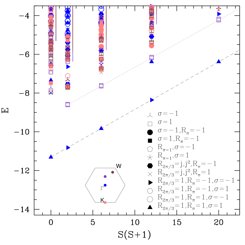
Figure 2.4: Antiferromagnetic Heisenberg model on the honeycomb lattice: eigen-energies vs eigen-values of ${\bf S}^{2}$. The dashed-line is a guide to the eyes for the QDJS. The dotted line joins the states associated to the first magnon. There is one QDJS for each $S$ (as expected for a collinear antiferromagnet): they are ${\bf k=0}$ states, invariant under a $2\pi/3$ rotation around an hexagon center, even (odd) under inversion, odd (even) under a reflection with respect to an axis going through nearest neighbor hexagon centers for $S$ even (odd) (taken from ref. [20]).

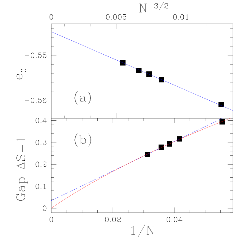
Figure 2.5: AF Heisenberg model on the honeycomb lattice, scaling of the QDJS with $S$ and $N$ for $N=18,24,26,28,32$ (taken from ref. [20]).

Figure 2.6: AF Heisenberg model on the honeycomb lattice, (a) energy per site $e_{0}$ versus $N^{-\frac{3}{2}}$ (b) spin-gap: The dashed line is a linear fit in $1/N$: for the sizes of interest the restriction to the leading term of the finite size expansion is insufficient. The full line is a fit to eq. [29, 31]: $\Delta(N)=\frac{1}{4\chi N}(1-\beta\frac{c}{\rho\sqrt{N}})+{\cal O}(\frac{1}{N^{2}})$ where $\chi$ is the spin susceptibility, $c$ is the spin-wave velocity, $\rho$ the spin stiffness and $\beta$ is a number of order one (taken from ref. [20]).

This global understanding of the spectra of finite size samples of antiferromagnets is a very useful tool to analyze exact spectra of spin models that can be obtained with present computer facilities . It seems that it may equally help to understand the time behavior of nano-scale antiferromagnets as ferritin [34].

2.2 A simple conceptual approach of the translational symmetry breaking of a solid

For a while we exclude any calculations and just rely on very simple and basic concepts of condensed matter physics and quantum mechanics to derive the “necessary” structure of the spectra of ordered condensed matter in finite size samples. For the sake of simplicity, we begin with the problem of the solid phase. We successively expose the fundamental classical hypothesis underlying the theory of solids. Quantization of this picture enlightens the translational symmetry breaking mechanism and finite size effects give a new light on the absence of solid order in 1-dimensional physics.

2.2.1 An essential classical hypothesis

Let us consider a finite sample of solid with $N$ atoms of individual mass m. The Hamiltonian of this piece of solid contains a kinetic energy term and an interaction term $U({\bf r}_{i}-{\bf r}_{j})$, which essentially depends on distances between the $N$ atoms, and is translation invariant. Nevertheless any piece of solid in nature breaks translational symmetry!

The first step in the description in classical phase space of the dynamics of this object with $2dN$ degrees of freedom, consists in sorting these variables in two sets:

• the center of mass variables: ${\bf R}_{c.o.m}$ and ${\bf P}_{c.o.m}$, the dynamics of which is a pure kinetic term ${\cal K}$:

  $${\cal K}=\frac{{\bf P}^{2}}{2Nm}$$ (2.18)

• and the $2d(N-1)$ internal variables, which obey a dynamic with interactions:

  $${\cal H}_{int}=\sum_{i\in[1,..,N]}\left[\frac{{\bf p_{i}}^{2}}{2m}+U({\bf r}_{i}-{\bf r}_{j})\right]$$ (2.19)

Then invoking the inertia principle, the analysis of the problem focuses on the Galilean frame, where the center of mass is at rest. In this frame, the internal excitations are analyzed in first approximation as modes of vibrations: the phonons, which present a dispersion law linear in ${\bf k}$ for small wave vectors ${\bf k}$.

In so doing, an essential dichotomy is introduced between the global variable and its dynamics on one hand and the internal excitations on the other: this dichotomy is at the basis of the concept of an ordered phase [9]. A technical asymmetry is also introduced in the treatment of the dynamics of these two sets of variables: the center of mass dynamics is described in a classical framework which explicitly breaks the translation invariance of the total Hamiltonian of the solid ${\cal K}+{\cal H}_{int}$. On the other hand the internal excitations are looked at in a translationally invariant (eventually quantum) point of view. This point of view may seem inconsistent in particular when looking at a finite sized, eventually small, piece of solid.

Taking as a definition of the solid phase the essential distinction between the global variable and the internal ones, we will show that the technical asymmetry in the treatment of these variables can be easily overcome, thus explaining both the localization of a piece of solid in real space, and the influence of space dimensionality on the definition of this solid.

2.2.2 Quantization of the classical approach, finite size spectra, thermodynamic limit and translational symmetry breaking

In order not to break artificially the translational symmetry of the problem we consider a solid with periodic boundary conditions.

If we take for granted that it is legitimate to disconnect the center of mass dynamics from the internal excitations we may consider a solid at $T=0$ with no internal excitations: the vacuum of phonons that we will write $|0>$.

The translationally invariant eigen-states of ${\cal K}$ are the plane waves with wave-vectors ${\bf k}$ where $k_{x,y,z}=n_{x,y,z}\frac{2\pi}{L}$, $L$ is the linear length of the sample and $n_{x,y,z}$ non zero integers. Their eigen-values are of the general form:

$${\frac{{\hbar}^{2}{\bf k}^{2}}{2mN}}.$$ (2.20)

The total energy of the solid in these states is thus of the form:

$$E_{0}(k)=\frac{{\hbar}^{2}{\bf k}^{2}}{2mN}+E_{g},$$ (2.21)

where $E_{g}$ is a constant measuring the zero point energy of the internal degrees of freedom. These eigen-states are shown in Fig. 2.7 connected by the red continuous line noted $|0>$.

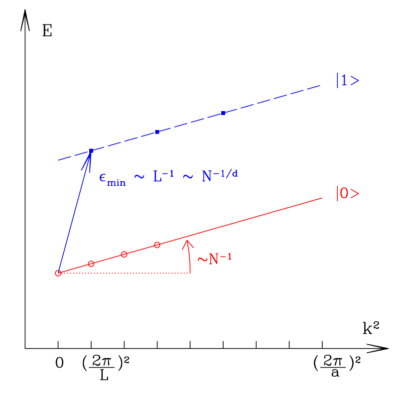
Figure 2.7: Typical spectrum of a finite size solid. The tower of eigen-levels joined by the continuous line and noted $\left|0\right>$ is the Anderson tower of states needed to form a symmetry breaking vacuum of phonons of the solid: such a state is non stationary on a finite size sample. The second set $\left|1\right>$ (dashed line) is associated with the lowest phonon.

In order to localize the center of mass it is necessary to form a wave-packet with eigen-states of ${\cal K}$ showing a large distribution of wave-vectors ${\bf k}$: the largest the ${\bf k}$-distribution be, the better the localization of the center of mass. Such a wave-packet is non stationary for a finite size, but its evolution rate goes to zero as ${\cal O}(1/N)$. Localization of the center of mass is thus a costless operation in the thermodynamic limit.

Let us look now to the first excitation of the solid with one phonon of wave vector ${\bf k}_{min}=2\pi/L$. This state can typically be written in a symmetry breaking picture as:

$$|1>=exp\left(\sum_{j}i{\bf k}_{min}.{\bf r}_{j}\right)|0>$$ (2.22)

It thus involves a linear superposition of eigenstates of ${\cal K}+{\cal H}_{int}$ with a distribution of wave vectors displaced by ${\bf k}_{min}$ with respect to the distribution of the localized ground-state $|0>$. This second set of excitations is displayed in Fig. 2.7 with a dashed line noted $|1>$ joining the different eigen-states. The softest phonon has an energy proportional to ${k}_{min}\propto L^{-1}\propto N^{-1/d}$ which should be added to the ground-state energy (2.21) giving eigen-states with eigen-energies:

$$E_{1}(k)=\frac{{\hbar}^{2}{\bf k}^{2}}{2mN}+E_{g}+{\hbar}ck,$$ (2.23)

where c is the sound velocity. Due to the structure of equation (2.23) the line joining the different translation invariant states of this soft phonon is parallel to the ground-state line $|0>$. This explains the supposed-to-be structure of the low lying levels of a finite size solid exhibited in Fig. 2.7.

2.2.3 Thermodynamic limit, stability of the solid and self-consistency of the approach

The consistency of the semi-classical picture implies that the localization of the center of mass could be done whatever the degree of excitations of phonons: looking to the finite size effects this appears to be the case if the dimension of space if larger or equal to 2. In these situations, for large enough sizes there appears two different scales of energy: the Anderson tower of states of the ground-state collapses as $N^{-1}$ to the absolute ground-state whereas the softest phonon collapses on the ground-state only as $N^{-1/d}$. In this limit, the dichotomy between the dynamics of the global variable and the internal variables is totally justified. On the other hand in 1 dimension it is quantum mechanically inconsistent to separate global degrees of freedom from internal ones: these two types of variables having dynamics that cannot be disentangled.

2.3 An analogy: $SU(2)$ symmetry breaking in the Néel antiferromagnet

Let us now develop the analogy between the solid states and the antiferromagnetic ones.

• The global variables of the solid are ${\bf R}_{c.o.m}$ and the conjugate variable ${\bf P}_{c.o.m}$. In the collinear antiferromagnetic case the global variables of position of the magnet are the two Euler angles $(\theta,\phi)$ allowing to point the direction of the sublattice magnetization in spin space. Their conjugate variable is the total spin operator ${\bf S}$.

• The free motion of the center of mass is governed by the Hamiltonian ${\cal K}$ (the quadratic form of this kinetic energy being related to the homogeneity of space). By analogy we expect the kinetic energy term describing the free precession of the sublattice magnetization to be of the form: ${\cal K}_{spin}={\bf S}^{2}_{tot}/2van$ . In such a point of view the constant a is just a multiplicative term: we know from other sources (fluctuation dissipation theorem or macroscopic approach of the magnet) that this is up to a constant the homogeneous spin susceptibility.

• The eigen-states describing the free precession of the order parameter in the vacuum of magnons are thus states with total spin $S$ (ranging from $0$ to $N/2$), and eigen-energies:

  $$E_{0}(S(S+1))=\frac{{\hbar}^{2}S(S+1)}{2\chi N}+E_{g}$$ (2.24)

  They form the set $|0>$ of Fig. 2.2. By forming a wave-packet out of this set one can localize the direction of the sublattice magnetization and break $SU(2)$ symmetry.

• The discussion of the first excitations above the vacuum of magnon completely parallelizes that of the phonons excitations (same dispersion law and same finite size scaling law). The eigen-energies of the states embedded in the softest magnon (referred as $|1>$ in Fig. 2.2) are thus of the form:

  $$E_{1}(S(S+1))=\frac{{\hbar}^{2}S(S+1)}{2\chi N}+E_{g}+{\hbar}c_{s}k_{min}$$ (2.25)

  where $c_{s}$ is the spin wave velocity.

• The possibility of a spin rotational symmetry breaking at the thermodynamic limit is embodied in the finite size behavior of the low lying levels of the spectra (Fig. 2.2). In dimension $d\geq 2$ the eigen-states of the sets $|0>$ (resp. $|1>$) collapse on their $S=S_{min}$ component as ${\cal O}(N^{{}_{-1}})$, more rapidly than the decrease in energy of the softest magnon which is ${\cal O}(N^{{}_{-1/2}})$. In dimension 2 and higher, the $SU(2)$ breaking mechanism prevails on the formation of magnon excitations justifying the classical approach and the dichotomy between global classical variables and internal excitations.

• These finite size scalings of the Anderson tower of states and of the true physical excitations (the magnons) give a new light on the Mermin Wagner theorem which denies the existence of Néel long range order in 1 dimensional magnets.

2.4 The coherent quantum mechanical description of the Néel state

At the end of this presentation I hope that Eq. (2.13) now appears as the natural quantum mechanical description of a coherent Néel state. And by the fact the usual symmetry breaking approach is justified as soon as it gives self consistent results (i.e. non zero order parameter).

The technical answer seems beyond doubt.

The question is now, do coherent states as those described in Eq. 1.11, which I rewrite here

$$|Qu.\;N\acute{e}el\;w.f.>=\sum_{S,M_{S}}{\frac{(-1)^{M_{S}}}{\sqrt{2S+1}}}\left(\begin{array}[]{ccc}S_{A}&S_{B}&S\\ S_{A}&-S_{B}&M_{S}\\ \end{array}\right)\widetilde{|S,M_{S}>}_{0}$$ (2.26)

exist in real life?

I see no mechanism which can lock the difference of phases of the macroscopic number of states $\widetilde{|S,M_{S}>}_{0}$ entering Eq. (2.26) to the correct values and it seems that many perturbations could destruct such a coherence, if, by an infinitesimal chance, it existed!

So I will plead that in real life the system may be in any incoherent superposition of the degenerate $\widetilde{|S,M_{S}>}_{0}$ which does not build in spin space a given direction to the sublattice magnetization!

But nobody has to care for it, experiments are not sensitive to the direction of the sublattice magnetizations but only to correlations functions: as the square of the staggered magnetization. This correlation function is identical in all the states of the Anderson tower in the Ising model; if it survives to quantum fluctuations introduced by ${\cal V}$, we expect it to be nearly identical in all the $\widetilde{|S,M_{S}>}_{0}$ states at least for total spin up to $S\sim\sqrt{N}$ (above these value of the total spin there might be some difficulties to disentangle magnons from the Anderson tower of states of the ground-state). This has been checked to be true in the Heisenberg model on the triangular lattice [10].

As a last remark, the homogeneous spin susceptibility is always dominated by the largest spin states of the Anderson tower: that is states with total spin ${\cal O}(\sqrt{N})$. Don’t forget that a state with total spin $\sqrt{N}$ has a macroscopic magnetization by site: $m=S_{tot}/\frac{N}{2}\propto\frac{1}{\sqrt{N}}$ that is essentially zero in the thermodynamic limit.

2.5 Space symmetry breaking of the Néel state.

The Néel state usually breaks some space symmetries of the lattice.

• In the square lattice case (see Fig. 2.3) one-step translations are not a symmetry operation of the ground-state but the point group is unbroken. This appears in the Anderson tower of states of Fig. 2.3, where the Irreducible Representations (IR) of the QDJS have alternatively wave-vector ${\bf k}=(0,0)$ or ${\bf k}=(\pi,\pi)$ (depending on the parity of the total spin), but are trivial IR of the point group.

• On the hexagonal lattice, which is not a Bravais lattice, the situation is somewhat different (see Fig. 2.6): the collinear Néel order does not break either the translation group, nor $C_{3}$, the group of 3-fold rotations (noted ${\cal R}_{\frac{2\pi}{3}}$). Only the trivial representation of these two groups appears in the QDJS (see Fig. 2.6). But both the inversion group ($C_{2}$, symmetry operation ${\cal R}_{\pi}$) and the reflection with respect to an axis joining the center of the hexagons ($\sigma$) are broken: these symmetry breakings appear in the Anderson tower where there is in the QDJS an alternation of even and odd IRs of these two groups.

Determination of the space symmetries of each $S$ components of the Anderson tower can be done exactly using symmetry arguments: the space symmetries of each $\widetilde{|S,M_{S}>}_{0}$ depend on $S$, on the shape and total number of spins of the sample [11, 35, 12, f03]. In the following chapter we will give an example of such a determination for the $J_{1}-J_{2}$ model on the triangular lattice. In a given range of parameters $1/8<J_{1}/J_{2}<1$, there is a competition between different orders and selection by quantum fluctuations of the more symmetric one. The study of this example will show the strength of the symmetry analysis and the exact nature of this phenomenon of “order by disorder”.

Chapter 3 “Order by disorder”

3.1 Some history

The concept of “order by disorder” was introduced in 1980 by Villain and co-workers[37] in the study of a frustrated Ising model on the square lattice. In this model the next neighbor couplings along all the rows are ferromagnetic as well as those on the odd columns (named A in the following). The couplings on the even columns (named B) are antiferromagnetic. It is assumed that

$$0\;<\;|J_{AB}|\;<\;J_{BB}\;<\;|J_{AA}|.$$ (3.1)

The ground-states of this model have A columns (resp B) ferromagnetically (resp. antiferromagnetically) ordered. For a system with a number of sites $N=0\;[{\rm mod}\,4]$, the degeneracy of this ground-state is $2^{\sqrt{N}}$, its entropy per spin $S_{0}=\frac{1}{\sqrt{N}}Ln2$ is negligible in the thermodynamic limit. At $T=0$ the ground-state has no average magnetization and is disordered. The picture changes when thermal fluctuations are introduced: it is readily seen that a B chain sandwiched between two A chains with parallel spins has lower excitations than a B chain sandwiched between two A chains with anti-parallel spins. This gives a larger Boltzmann weight to the ferrimagnetically ordered system. Villain and co-workers have been able to show exactly that the system is indeed ferrimagnetic at low $T$. They were equally able to show that site dilution (introducing non magnetic species) was in a certain domain of composition and temperature able to select the same ordered pattern, whence the name of “order by disorder”.

During the nineties several authors have studied a somewhat less drastic problem in the classical or quantum Heisenberg model : it is the selection of a special kind of long range order among a larger family of ordered solutions classically degenerate at T=0 [38, 39, 40, 41, 42, 43, 44]. In the classical models, the selection of the simplest ordered structure by thermal fluctuations , is due to a larger density of low lying excitations around these solutions, whence an increased Boltzmann weight of the corresponding regions and a thermal (entropic) selection of order.

This same property of the density of low lying excitations can also explain a selection of specific spin configurations when going from the $T=0$ classical approach of the Heisenberg model to the semi-classical one. Suppose that many classical spin configurations are degenerate in the classical limit, the existence of a larger density of excitations around a specific configuration is the signature of a weaker restoring force toward this configuration (larger well width in phase space). Insofar as the semi-classical spin-wave approach is valid, this implies that the zero point quantum energy $\sum_{{\bf q}\in BZ^{*}}\frac{\omega_{\bf q}}{2}$ of Eq. 2.15 is smaller for this solution, which will thus be energetically selected by the “quantum” fluctuations. Both mechanisms (thermal or quantum) lay on the properties of the low lying excitations around the classically $T=0$ degenerate solutions.

This selection of order is, in most of the cases, less drastic in the continuous spin models, than in the original problem of Villain. In most of the cases, the degeneracy of the ground-state is less severe than in the Villain case. In the Ising domino problem, the degeneracy of the ground-state is $2^{\sqrt{N}}$ and the thermal selection emphasizes 4 ground-states among these $2^{\sqrt{N}}$. In the Heisenberg problem, as we will see below, in most of the cases the less ordered solution has a degeneracy of order ${\cal O}(N^{\alpha})$, with $\alpha$ the number of sublattices, whereas the final order selected by quantum fluctuations has only a degeneracy ${\cal O}(N^{\beta})$ with $\beta<\alpha$. From that simple point of view one can qualitatively state that the selection of order is less drastic than in the Villain problem. A special mention should be done of the Heisenberg model on the kagome, checker-board or pyrochlore lattices. In these cases, on which we will return at the end of these lectures, the degeneracy of the classical ground-state is exponential in $N$, there is a residual entropy per spin at $T=0$ and a selection (if any) of some partial order is a more difficult issue.

3.2 ”Order by disorder” in the $J_{1}-J_{2}$ model on the triangular lattice

The existence of competing interactions is indeed the main cause of classical ground-states degeneracy. As a generic example, one can consider the so-called $J_{1}-J_{2}$ model on a triangular lattice with two competing antiferromagnetic interactions. This Hamiltonian reads:

$${\cal H}=2J_{1}\sum_{<i,j>}{\bf S}_{i}.{\bf S}_{j}+2J_{2}\sum_{<<i,k>>}{\bf S}_{i}.{\bf S}_{k}$$ (3.2)

where $J_{1}$ and $J_{2}=\alpha J_{1}$ are positive and the first and second sums run on the first and second neighbors, respectively. The classical study of this model has been developed by Jolicoeur et al. [42]. They have shown that for small $\alpha$ ($\alpha<1/8$) the ground state corresponds to a three-sublattice Néel order with magnetizations at $120^{o}$ from each other, whereas for $1/8<\alpha<1$, there is a degeneracy between a two-sublattice Néel and a four-sublattice Néel order (see Fig. 3.1). Chubukov and Jolicoeur [43] and Korshunov [44] have then shown that quantum fluctuations (evaluated in a spin wave approach) could, like thermal ones, lift this degeneracy of the classical ground states and lead to a selection of the collinear state (see Fig. 3.1) [45].

Figure 3.1: Top: 4-sublattice classical ground state. Spins in the sublattices $A$ and $B$, as well as spins in $C$ and $D$, make an angle $2\theta$. The plane of the spins of $A$ and $B$ makes an angle $\phi$ with the plane of the spins of $C$ and $D$. Bottom: the collinear solutions with the three possible arrangements (in this case, classical spins in sublattices A and B are antiparallel).

The first study of the exact spectrum of Eq. (3.2) done by Jolicoeur et al. was not incompatible with this conclusion, but was insufficient to yield it immediately. I will show now how the study of the degeneracy of the Anderson tower allows a direct derivation of this phenomenon. This part of the lecture closely follows the paper by Lecheminant e͡t al.[35].

As we have done in section (2.1), let us first study the exactly solvable models which display either four-sublattice order or collinear order. These models are obtained by extracting from the Heisenberg Hamiltonian expressed in terms of the Fourier components of the spin:

$${\cal H}=6J_{1}\sum_{\bf k}{\bf S}_{\bf k}.{\bf S}_{-\bf k}\left[\gamma_{\bf k}+\frac{\alpha}{3}\left(\cos{\bf k}.\left(2{\bf u}_{1}+{\bf u}_{2}\right)+\cos{\bf k}.\left({\bf u}_{1}+2{\bf u}_{2}\right)+\cos{\bf k}.\left({\bf u}_{2}-{\bf u}_{1}\right)\right)\right],$$ (3.3)

where $\gamma_{\bf k}=1/3\sum_{\mu}\cos{\bf k}.{\bf u}_{\mu}$ (${\bf u}_{\mu}$ are three vectors at 120 degrees from each other and connecting a given site to first neighbors), those which describe either the 4-sublattice structure or the collinear ones.

3.2.1 Symmetry analysis of the Anderson tower of the 4-sublattice Néel order.

The four ${\bf k}$ vectors which keep the four-sublattice order invariant are ${\bf k}={\bf 0}$ and the three middles of the Brillouin zone boundaries (called in the following $\bf k_{I}$, $\bf k_{H}$ and $\bf k_{G}$). It is straightforward to write the contribution of these Fourier components to ${\cal H}$ in the form:

$${}^{4}{\cal H}_{0}=\frac{8}{N}\left(J_{1}+J_{2}\right)\left({\bf S}^{2}-{\bf S}_{A}^{2}-{\bf S}_{B}^{2}-{\bf S}_{C}^{2}-{\bf S}_{D}^{2}\right),$$ (3.4)

where ${\bf S}$ is the total spin operator and ${\bf S}_{\alpha}$ are the total spin operator of each sublattice. ${}^{4}{\cal H}_{0},{\bf S}^{2},{\bf S}_{A}^{2},{\bf S}_{B}^{2},{\bf S}_{C}^{2}$ and ${\bf S}_{D}^{2}$ form a set of commuting observables. The eigenstates of ${}^{4}{\cal H}_{0}$ have the following energies:

$$\begin{array}[]{clc}{}^{4}E(S,S_{A},S_{B},S_{C},S_{D})=&\displaystyle\frac{8}{N}\left(J_{1}+J_{2}\right)\left[S(S+1)-S_{A}\left(S_{A}+1\right)\right.\\ &\left.\displaystyle-S_{B}\left(S_{B}+1\right)-S_{C}\left(S_{C}+1\right)-S_{D}\left(S_{D}+1\right)\right]\end{array}$$ (3.5)

where the quantum numbers $S_{A},S_{B},S_{C},S_{D}$ run from $0$ to $N/8$ and the total spin results from a coupling of four spins $S_{A},S_{B},S_{C},S_{D}$.

The low lying levels of Eq. 3.5 are obtained for $S_{A}=S_{B}=S_{C}=S_{D}=N/8$:

$${}^{4}E_{0}(S)=-\frac{J_{1}+J_{2}}{2}\left(N+8\right)+\frac{8}{N}\left(J_{1}+J_{2}\right)S\left(S+1\right).$$ (3.6)

These states, which have maximal sublattice magnetizations $S_{A}^{2}=S_{B}^{2}=S_{C}^{2}=S_{D}^{2}={\frac{N}{8}}(\frac{N}{8}+1)$, are the rotationally invariant projections of the bare Néel states with four sublattices. Their total energy collapses to the absolute ground-state as $N^{-1}$ and form the Anderson tower of the 4-sublattice Néel order (noted $\{^{4}\tilde{E}\}$ in the following).

As we will now show, this multiplicity $\{^{4}\tilde{E}\}$ can be entirely and uniquely described by its symmetry properties under spin rotations and transformations of the space group of the lattice.

Let us begin by the SU(2) properties of $\{^{4}\tilde{E}\}$. These states result from the coupling of four identical spins of length $N/8$. There is $N_{S}$ different ways to couple these 4 spins: the degeneracy of each $S$ subspace is thus $(2S+1)N_{S}$, where the $(2S+1)$ factor comes from the magnetic degeneracy of each $S$ eigen-state. $N_{S}$ is readily evaluated by using the decomposition of the product of four spin $N/8$ representations of $SU(2)$ (${\cal D}^{N/8}$)

$$\{^{4}\tilde{E}\}={\cal D}^{N/8}\otimes{\cal D}^{N/8}\otimes{\cal D}^{N/8}\otimes{\cal D}^{N/8}$$ (3.7)

in spin $S$ irreducible representations (${\cal D}^{S}$). One obtains:

$$N_{S} = \frac{1}{2}\left(-3S^{2}+S\left(N+1\right)+2+\frac{N}{2}\right)~{}~{}~{}~{}{\rm for~{}~{}~{}}S\leq\frac{N}{4},$$ (3.8)

$$= \frac{1}{2}\left(\frac{N}{2}-S+1\right)\left(\frac{N}{2}-S+2\right)~{}~{}~{}~{}{\rm for~{}~{}~{}}S\geq\frac{N}{4}+1.$$ (3.9)

Note that this degeneracy depends both on $S$ and $N$ and not only on the total spin $S$ as is the case for a two or three-sublattice problem.

The determination of the space symmetries of these eigenstates allows a complete specification of $\{^{4}\tilde{E}\}$.

• The four-sublattice order is invariant in a two-fold rotation: the eigenstates of $\{^{4}\tilde{E}\}$ belong to the trivial representation of $C_{2}$.

• $\{^{4}\tilde{E}\}$ forms a representation of $S_{4}$, the permutation group of four elements. The eigenstates of $\{^{4}\tilde{E}\}$ could thus be labeled by the irreducible representations (I.R.) of $S_{4}$ (see Table 3.1).

  $S_{4}$	$I$	$(A,B)(C,D)$	$(A,B,C)$	$(A,B)$	$(A,B,C,D)$
  ${\cal G}$	$I$	$t$	${\cal R}_{2\pi/3}$	$\sigma$	${\cal R}^{{}^{\prime}}_{2\pi/3}\sigma$
  $N_{el}$	1	3	8	6	6
  $\Gamma_{1}$	$1$	$1$	$1$	$1$	$1$
  $\Gamma_{2}$	$1$	$1$	$1$	$-1$	$-1$
  $\Gamma_{3}$	$2$	$2$	$-1$	$0$	$0$
  $\Gamma_{4}$	$3$	$-1$	$0$	$1$	$-1$
  $\Gamma_{5}$	$3$	$-1$	$0$	$-1$	$1$

  Table 3.1: Character table of the permutation group $S_{4}$. First line indicates classes of permutations. Second line gives an element of the space symmetry class corresponding to the class of permutation. These space symmetries are: the one step translation $t$ ($A\to C$), ${\cal R}_{2\pi/3}$ (resp. ${\cal R}^{{}^{\prime}}_{2\pi/3}$) the three-fold rotation around a site of the $D$ (resp. $B$) sublattice, and $\sigma$ the axial symmetry keeping invariant $C$ and $D$. $N_{el}$ is the number of elements of each class.

• Each element of the space group maps onto a permutation of $S_{4}$ : one step translations onto products of transpositions as $(AC)(BD)$, three-fold rotations onto circular permutations of three sublattices $(ABC)$ and so on. The complete mapping of the space symmetries of the four-sublattice order onto the permutations of $S_{4}$ is given in Table 3.1 together with the character table of $S_{4}$.

• Each irreducible representation of $S_{4}$ can thus be characterized in terms of its space symmetry properties. As noted above they are all invariant in $\cal{R_{\pi}}$. $\Gamma_{1},\Gamma_{2},\Gamma_{3}$ belong to the trivial IR of the translation group, characterized by the wave-vector ${\bf 0}$, whereas $\Gamma_{4}$ and $\Gamma_{5}$ have a wave-vector ${\bf k}_{H},{\bf k}_{I}$ or ${\bf k}_{G}$. $\Gamma_{1}$ and $\Gamma_{2}$ belong to the trivial I.R. of $C_{3}$, whereas $\Gamma_{3}$ is the 2 dimensional representation of this same group. Finally, $\Gamma_{1}$ and $\Gamma_{4}$ are even under axial symmetry, whereas $\Gamma_{2}$ and $\Gamma_{5}$ are odd.

• The number of replicas of $\Gamma_{i}$ that should appear for each $S$ is then computed in the $S,M_{S}$ subspace with the help of the trace of the permutations of $S_{4}$:

  $$n_{\Gamma_{i}}^{(S)}=\frac{1}{24}\sum_{l}{\rm Tr}(R_{l}|_{S})\chi_{i}(l)N_{\rm el}(l)$$ (3.10)

  where $R_{l}$ is an element of the class $l$ of $S_{4}$, $N_{\rm el}(l)$ is the number of elements of the group in this class and $\chi_{i}(l)$ the character of the class $l$ in the I.R. $\Gamma_{i}$ (see Table 3.1). The values of the traces for a given total spin $S$ are then found as:

  $${\rm Tr}\left(R_{l}\bigg{|}_{S}\right)={\rm Tr}\left(R_{l}\bigg{|}_{M_{S}=S}\right)-{\rm Tr}\left(R_{l}\bigg{|}_{M_{S}=S+1}\right).$$ (3.11)

  In each $M_{S}$ subspace of $\{^{4}\tilde{E}\}$ , it is straightforward to find the trace of the elements of $S_{4}$:

  $${\rm Tr}\left(I_{d}\bigg{|}_{M_{S}}\right) = \sum_{t,v,x,y=-N/8}^{N/8}\delta_{t+v+x+y,M_{S}}$$

  $${\rm Tr}\left(\left(A,B\right)\left(C,D\right)\bigg{|}_{M_{S}}\right) = \sum_{t,v=-N/8}^{N/8}\delta_{2t+2v,M_{S}}$$

  $${\rm Tr}\left(\left(A,B,C\right)\bigg{|}_{M_{S}}\right) = \sum_{t,v=-N/8}^{N/8}\delta_{3t+v,M_{S}}$$ (3.12)

  $${\rm Tr}\left(\left(A,B\right)\bigg{|}_{M_{S}}\right) = \sum_{t,v,x=-N/8}^{N/8}\delta_{2t+v+x,M_{S}}$$

  $${\rm Tr}\left(\left(A,B,C,D\right)\bigg{|}_{M_{S}}\right) = \sum_{t=-N/8}^{N/8}\delta_{4t,M_{S}}$$

  where $t,v,x,y$, are the $z$-components of the total spin of each sublattice (constrained to vary between $N/8$ and $-N/8$) and $\delta_{i,j}$ denotes the Kronecker symbol. Using equations (3.10, 3.11, 3.12) one readily obtains the number of occurrences of each $\Gamma_{i}$ for any $S$ subset of $\{^{4}\tilde{E}\}$ (Table 3.2). Note that this result depends on $S$ and on the size of the sample.

  $N=16$
  $S$	0	1	2	3	4	5	6	7	8
  $n_{\Gamma_{1}}(S)$	1	0	2	0	2	1	1	0	1
  $n_{\Gamma_{2}}(S)$	0	0	1	0	0	0	0	0	0
  $n_{\Gamma_{3}}(S)$	2	0	2	1	2	0	1	0	0
  $n_{\Gamma_{4}}(S)$	0	2	2	3	2	2	1	1	0
  $n_{\Gamma_{5}}(S)$	0	2	1	2	1	1	0	0	0

  $N=28$
  $S$	0	1	2	3	4	5	6	7	8	9	10	11	12	13	14
  $n_{\Gamma_{1}}(S)+n_{\Gamma_{2}}(S)$	2	0	5	1	5	3	4	2	4	1	2	1	1	0	1
  $n_{\Gamma_{3}}(S)$	3	0	4	2	5	2	5	2	3	1	2	0	1	0	0
  $n_{\Gamma_{4}}(S)+n_{\Gamma_{5}}(S)$	0	7	6	11	9	12	9	10	6	6	3	3	1	1	0

  Table 3.2: Number of occurrences $n_{\Gamma_{i}}(S)$ of each irreducible representation $\Gamma_{i}$ with respect to the total spin $S$. For $N=28$, $n_{\Gamma_{1}}$ and $n_{\Gamma_{2}}$ as well as $n_{\Gamma_{4}}$ and $n_{\Gamma_{5}}$ have been added because this sample does not present any axial symmetry.

This symmetry analysis completes the determination of the QDJS of $\{^{4}\tilde{E}\}$. These properties of the Anderson tower are stable under the action of the discarded part of the Heisenberg Hamiltonian. If the ordering of levels is not destroyed by quantum fluctuations, the associated quantum numbers remain good quantum numbers of the low lying levels $\widetilde{|S,M_{S}>}_{0}$ of the $J_{1}-J_{2}$ model (3.2). We have thus obtained the complete determination (all quantum numbers , and all the degeneracies) of the family of low lying levels describing the ground-state multiplicity $\{^{4}\tilde{E}\}$ of the four-sublattice Néel solutions.

3.2.2 Symmetry analysis of the QDJS of the Anderson tower of states of the 2-sublattice collinear solutions.

Let us now consider the collinear solutions (Fig. 3.1). They are particular solutions of the 4-sublattice case and we will rapidly get through the same scheme of analysis, indicating mainly the new points. The two vectors which keep the two sublattices invariant are ${\bf 0}$ and the middle of one side of the Brillouin zone (the vectors $\bf{k_{I}}$, $\bf{k_{H}}$ and $\bf{k_{G}}$ correspond respectively to the collinear solutions $(a)$, $(b)$ and $(c)$ in Fig. 3.1). Extracting a specific set of two wave-vectors from Eq. 3.3, we find the following contribution to the total Hamiltonian:

$${}^{2}{\cal H}_{0}=\frac{8}{N}\left(J_{1}+J_{2}\right)\left[{\bf S}^{2}-\frac{1}{2}\left({\bf S}_{\alpha}^{2}+{\bf S}_{\beta}^{2}\right)\right].$$ (3.13)

The corresponding low energy spectrum for $S_{\alpha}=S_{\beta}=N/4$ is:

$${}^{2}E_{0}(S)=-\frac{J_{1}+J_{2}}{2}\left(N+8\right)+\frac{8}{N}\left(J_{1}+J_{2}\right)S\left(S+1\right)$$ (3.14)

and is degenerate with the four-sublattice low energy spectrum (see Eq. 3.6). But here the two-sublattice have maximal spins $S_{\alpha}=S_{\beta}=N/4$. These new solutions arise from the three symmetric couplings of the 4-sublattice spins: $\bf{S}_{\alpha}=\bf{S}_{A}+\bf{S}_{B}$ or $\bf{S}_{\alpha}=\bf{S}_{A}+\bf{S}_{C}$ or $\bf{S}_{\alpha}=\bf{S}_{A}+\bf{S}_{D}$ with the symmetric counterparts for $\bf{S}_{\beta}$. These collinear solutions have thus a $Z_{3}$ degeneracy (see Fig. 3.1). The representation space is thus the sum of three products ${\cal D}^{N/4}\otimes{\cal D}^{N/4}$. It is not a direct sum since ${\cal D}^{N/4}(A,B)\otimes{\cal D}^{N/4}(C,D)$ and ${\cal D}^{N/4}(A,C)\otimes{\cal D}^{N/4}(B,D)$ have in common the same (symmetric) irreducible representation with a total spin $N/2$. On an $N$-sample, the representation space of the ground state of the collinear solution is:

$$\{^{2}\tilde{E}\}=3{\cal D}^{S=0}\oplus 3{\cal D}^{S=1}\oplus....\oplus 3{\cal D}^{S=N/2-1}\oplus{\cal D}^{S=N/2}.$$ (3.15)

The degeneracy is thus $3(2S+1)$ for all $S$ values except for $S=N/2$, where it is only $(2S+1)$.

The space group analysis is identical to the analysis done for the four-sublattice order, but the number of occurrences of each I. R. $\Gamma_{i}$ is now different , since the space $\{^{2}\tilde{E}\}$ is smaller than $\{^{4}\tilde{E}\}$. For each $S$ value there are only three replicas of ${\cal D}^{S}$ arising from the $Z_{3}$ symmetry ( Eq. 3.15 and Fig. 3.1). This allows the direct computation of the traces of the operations of $S_{4}$ in each $S$ subset of $\{^{2}\tilde{E}\}$. Using the coupling rules of two angular momenta (and in particular the fact that the $S$ eigen-state resulting from the coupling of two integer spins changes sign as $(-1)^{S}$ with the interchange of the two parent spins) one obtains (for $S\neq N/2$):

$$\left\{\begin{array}[]{l}\displaystyle{\rm Tr}\left(I_{d}|_{S}\right)=3\\ \displaystyle{\rm Tr}\left(\left(A,B\right)\left(C,D\right)|_{S}\right)=1+2\left(-1\right)^{S}\\ \displaystyle{\rm Tr}\left(\left(A,B,C\right)|_{S}\right)=0\\ \displaystyle{\rm Tr}\left(\left(A,B\right)|_{S}\right)=1\\ \displaystyle{\rm Tr}\left(\left(A,B,C,D\right)|_{S}\right)=\left(-1\right)^{S}\end{array}\right.$$ (3.16)

Therefore the collinear solution is simply characterized by $\Gamma_{1}$ and $\Gamma_{3}$ for even $S$, and $\Gamma_{4}$ for odd $S$, whatever the sample size.

The symmetries of all states of the tower are now fully determined both for the 4-sublattice order $\{^{4}\tilde{E}\}$ and for the collinear order $\{^{2}\tilde{E}\}$. If the quantum Hamiltonian presents one of these kinds of order, the quantum fluctuations generated by the discarded part of $\cal H$ should preserve the dynamics and the structure of these low lying subsets.

3.2.3 Exact spectra of the $J_{1}-J_{2}$ model on small samples and finite size effects: a direct illustration of the phenomenon of “order by disorder”.

We have determined the low (and high) energy levels of the $J_{1}-J_{2}$ Hamiltonian in each I. R. of $SU(2)$ and of the space group of the triangular lattice for small periodic samples with $N=12,16$ and $N=28$. The spectra are displayed in Fig. 3.2 and Fig. 3.3.

Figure 3.2: Top: complete spectrum of the $N=16$ periodic sample with respect to ${\bf S}^{2}$. Bottom: enlargement of the difference between the exact spectrum and the energy of the low lying levels of the model Hamiltonians (Eq.3.6 or Eq.3.14). The ground-state multiplicity $\{^{4}\tilde{E}\}$ is well separated from the magnons.

Figure 3.3: Partial spectrum of the $N=28$ periodic sample. (Same legend as for fig.3.2). Bottom: the tower of states of the 4-sublattice order $\{^{4}\tilde{E}\}$ lays under the dashed line. Above appear the first magnons. Above the dotted line are represented the first excited homogeneous states. In the magnon multiplicity ($\bf k\neq\bf 0,{\bf k_{H}},{\bf k_{I}}$ or ${\bf k_{G}}$), for $S\leq 5$, only the lowest 5 states of each I.R. have been computed.

We directly see in the upper parts of these figures the set of QDJS (”Anderson tower of the ground-state”) well separated from the set of levels corresponding to the one magnon excitations. We have verified that this set has the symmetry properties of the above defined $\{^{4}\tilde{E}\}$ subset. The action of the quantum fluctuations could then be read in the lower parts of the figures. As expected, the quantum fluctuations lift the degeneracies which are present in the exactly solvable model and stabilize the eigenstates with the lower $S$ values. Nevertheless the low lying energies per site still group around a line of slope ${\cal O}[(J_{1}+J_{2})/N^{2})$. The number and space symmetries of these levels for each $S$ and $N$ value are exactly those required by the above analysis of the four-sublattice Néel order.

Moreover, it is already visible on the $N=16$ sample and quite clear on the $N=28$ sample that a dichotomy appears in this family (see Fig. 3.4). The lowest levels of this tower of states appear to be $\Gamma_{1},\Gamma_{3}$ or $\Gamma_{4}$ representations depending on the parity of the total spin. They precisely build the family $\{^{2}\tilde{E}\}$ of isotropic projections of the collinear solutions (Eq. 3.16).

Figure 3.4: Enlargement of the $N=16$ and $N=28$ QDJS. A global contribution $\beta E_{0}(S)$ is subtracted from the exact spectrum. This contribution describes the overall dynamics of the order parameter in this finite sample, $\beta$ measures the renormalization of this dynamics by quantum fluctuations (see refs. [11, 35]). The bars represent eigenstates which belong both to $\{^{2}\tilde{E}\}$ and $\{^{4}\tilde{E}\}$. The triangles indicate states which belong to $\{^{4}\tilde{E}\}$ but not to $\{^{2}\tilde{E}\}$. With increasing sizes, the subset $\{^{2}\tilde{E}\}$ is stabilized and separates from the pure 4-sublattice order. For $N=28$ the two states of $\{^{2}\tilde{E}\}$ with even $S$ are quasi degenerate and cannot be distinguished at the scale of the figure.

This strongly suggests that the 4-sublattice order will disappear in the thermodynamic limit and only the collinear order will subsist, as was predicted in the spin-wave approach [42, 43, 44].

3.3 Concluding remarks

• The symmetry and dynamical analysis of the low lying levels of a Hamiltonian likely to exhibit ordered solutions gives rather straightforward answer to the kind of order to be expected. The method is rapid, powerful and unbiased. It does not require any a priori symmetry breaking choice: if a specific order is selected, one should see it directly on the exact spectra. Moreover, as it is essentially exact, there are no questions relative to the convergence of the expansion as in the spin-wave approach. On the other hand, as the sizes amenable to computation are limited, there is, in the exact approach, a cut-off of the long wavelength fluctuations. Results so obtained should thus be examined in the light of a finite size scaling analysis. This work nevertheless shows that it is not necessary to invoke quantum fluctuations with very long wave-lengths to select the collinear order.

• The selection of “order by disorder” appears in a particular clear light. Increasing the sample size, increases the presence of long wave-length fluctuations. We see on this example how these long wave-length fluctuations realize a differential stabilization of the $\{^{2}\tilde{E}\}$ subset, favoring collinear order and progressively wiping out 4-sublattice order. This fully support the spin-wave calculations. This is also a clear illustration of the previous comment on the “non drastic” character of this phenomenon in this peculiar case. Without fluctuations the system has already some order: the role of the quantum fluctuations is just to restore a higher degree of symmetry to the ground-state solution.

• Going along this route one may always speculate if in the thermodynamic limit, quantum fluctuations could not completely restore the symmetries of the Hamiltonian. Spin-waves calculations, so long they are consistent at small sizes with exact diagonalizations and self-consistent when going to the thermodynamic limit are credible. This comparison is always useful and relevant: in the $J_{1}-J_{2}-J_{3}$ model on the hexagonal lattice [20, f03], there are regions of parameter space where finite-size exact diagonalizations give Néel Long Range Order whereas spin-waves in the thermodynamic limit indicate an absence of sublattice magnetization! We have verified in each of these cases that at small sizes the semi-classical solution in the spin-wave approach was equally robust and was only destroyed by very long wave-length fluctuations.

• On the other hand, in the situations where we claim an absence of Néel Long Range Order and a more exotic phase (see next chapters on Valence Bond Crystals and Resonating Valence Bond Spin Liquids) the Anderson tower of states is absent even on the smallest sizes. In such a case it is quite clear that the spin-wave approach should be discarded for spin-1/2.

Chapter 4 Valence Bond Crystals

4.1 Introduction

In our quest of exotic quantum ground-states, we will now describe some examples where the semi-classical Néel order is not the ground-state of the problem and $SU(2)$ symmetry is not broken.

In this chapter we will concentrate on solutions where there is long range order in the dimer coverings: we call these phases Valence Bond Crystals (in the following noted VBC).

Such solutions are well known in 1-dimensional problems as for example in the A.F. $J_{1}-J_{2}$ model:

$${\cal H}=J_{1}\sum_{<ij>}{\bf S}_{i}.{\bf S}_{j}+J_{2}\sum_{<<ij>>}{\bf S}_{i}.{\bf S}_{j}$$ (4.1)

where the first (resp. second) sums run on first (resp. second) neighbors. In 1-d, for $J_{2}/J_{1}>0.24$, the ground-state is dimerized and there is a gap to the first excitations: this is the simplest case of a VBC.

What is the situation in 2-d?

In a classical approach, the ground-state of Eq. (4.1) on a square lattice has a soft mode at $(\pi,\pi)$ for $J_{2}/J_{1}<0.5$. At $J_{2}/J_{1}=0.5$, the $(\pi,\pi)$ order is degenerate with 4-sublattice order and collinear $(\pi,0)$ or $(0,\pi)$ order. For $J_{2}/J_{1}>0.5$, quantum fluctuations select the collinear $(\pi,0)$ or $(0,\pi)$ order by the phenomenon of “order by disorder” (see Fig. 4.1).

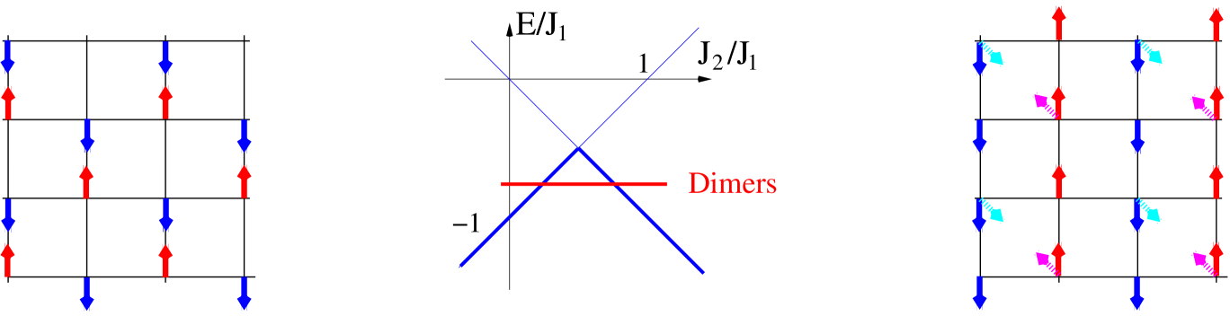
Selection of order by disorder
                                                        & Restoration of symmetry by fluct.

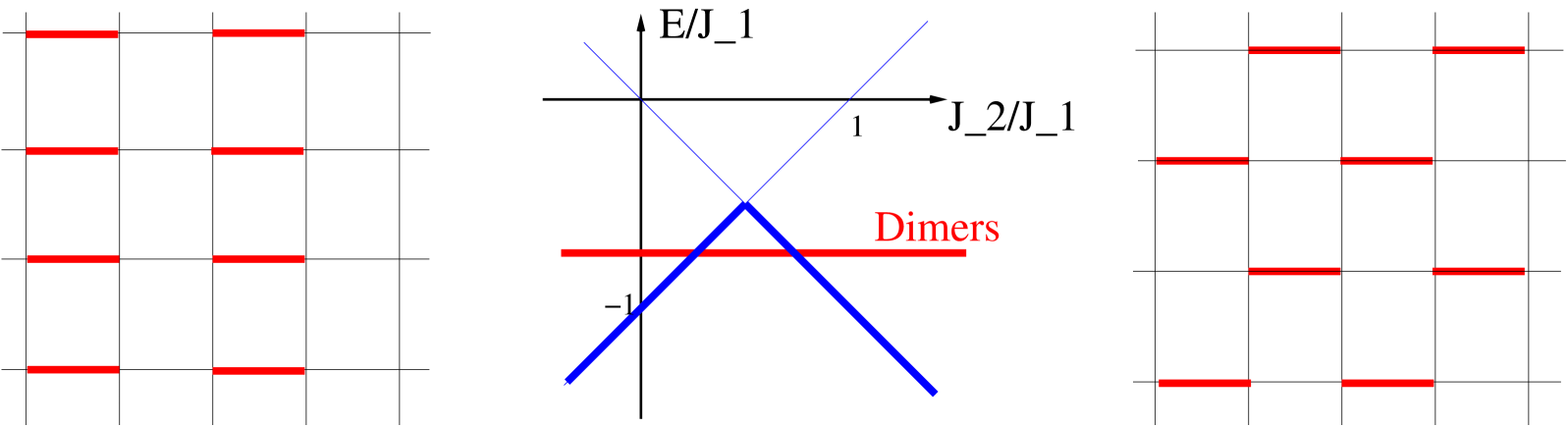
columnar VBC                                                                  staggered VBC

Figure 4.1: Schematization of different variational solutions of the $J_{1}-J_{2}$ model described in the introduction of this chapter

In our naive approach of chapter 1, comparing the energies of classical Néel solutions to dimer covering ones, we would conclude that dimer covering solutions and VBC are more stable than any classical Néel order in a large range of parameters around $J_{2}/J_{1}=0.5$ (Fig. 4.1).

In fact “quantum fluctuations” stabilize the Néel states and the window for an exotic phase is smaller than indicated in Fig. 4.1. The nature of the quantum phase on the square lattice at $J_{2}/J_{1}=0.5$ is still debated [46, 47, 48, 49, 50, 51]. A columnar VBC has been identified in the same model on the honeycomb lattice for $J_{2}/J_{1}\sim 0.4$ (see ref. [20] and refs. therein). For a pedagogical illustration we will move to a more clear-cut example: the Heisenberg model on the checkerboard lattice [52, fmsl03] (noted in the following HCKB).

4.2 The Heisenberg model on the checker-board lattice: an example of a Valence Bond Crystal

The checker-board lattice is made of corner sharing tetrahedrons, with all bonds equal: this a 2-dimensional slice of a pyrochlore lattice. The underlying Bravais lattice is a square lattice and there are two spins per unit cell (Fig. 4.2).

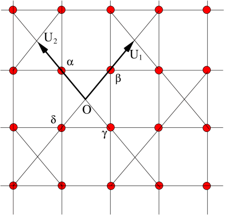
Figure 4.2: The checkerboard lattice: the spins sit at the vertices shown by bullets, all couplings are identical, $\bf u_{1},u_{2}$ are the unit vectors of the Bravais lattice.

4.2.1 Classical ground-states

The Heisenberg Hamiltonian on such a lattice is highly degenerate in the classical limit. Due to the special form of the lattice this Hamiltonian can be rewritten as the sum of the square of the total spin of corner sharing units $\alpha$ :

$${\cal H}=J\sum_{(i,j)\,bonds}{\bf S}_{i}.{\bf S}_{j}\equiv\frac{J}{2}\sum_{\alpha\,units}{\bf S_{\alpha}}^{2}-\frac{NJ}{4}.$$ (4.2)

A classical ground-state is obtained whenever $\forall\alpha\hskip 8.5359pt{\bf S_{\alpha}}=0$. Such ground-states have a continuous local degeneracy and an energy $-(NJ)/4$. This is much higher than the dimer covering energy, which is $-(3NJ)/8$. As we will see below, there is no memory of these classical solutions in the quantum ground-states and low lying excitations of this model.

Figure 4.3: Gap between the absolute ground-state and the first S=1 excitation of the HCKB model versus sample sizes.

4.2.2 The Quantum HCKB model: Spin Gap

As we have seen in chapter 2, the first characteristic of the semi-classical Néel like solution is the existence of the Anderson tower of states which collapse to the ground-state as ${\cal O}(1/N)$ and the absence of spin gap in the thermodynamic limit (see for example Fig. 2.6).

The first salient feature of the Heisenberg model on the checker-board lattice is the existence of a large spin gap, which shows no tendency of going to zero at the thermodynamic limit (compare Fig. 4.3 with Fig. 2.6). This indicates that the ground-state does not break the $SU(2)$ symmetry of the Hamiltonian, and as a corollary we expect that the spin-spin correlations decrease to zero at large distance (which seems well verified, see Table IV of ref. [fmsl03]).

4.2.3 Degeneracy of the ground-state and space symmetry breaking in the thermodynamic limit

The low lying levels of the spectra of the HCKB model in the singlet space are displayed in Fig. 4.4.

Figure 4.4: Gaps to the first (open up triangles) and second (black squares) level of the singlet sector. For the studied samples these two “excited” singlet levels are in the singlet-triplet gap (See Fig. 4.3).

In this figure, one reads that the first excited singlet state very plausibly collapses to the absolute ground-state, whereas a finite gap to the third S=0 level (perhaps smaller than the spin gap) build on with sample size. This pleads in favor of a 2-fold degeneracy of the absolute ground-state in the thermodynamic limit.

The absolute ground-state is in the trivial representation of the lattice symmetry group. Its wave function is invariant in any translation and in any operation of $D_{4}$: group of the $\pi/2$ rotations around point O (or any equivalent point of the Bravais lattice) and axial symmetries with respect to axes $\bf u_{1}$ and $\bf u_{2}$ (see Fig. 4.2). The excited state which collapses on it in the thermodynamic limit has a wave vector $(\pi,\pi)$ (its wave function takes a (-1) factor in one-step translations along $\bf u_{1}$ or $\bf u_{2}$), and it is odd under $\pi/2$ rotations and axial symmetries. In the thermodynamic limit the 2-fold degenerate ground-state can thus exhibit a spontaneous symmetry breaking with a doubling of the unit cell.

Such a restricted symmetry breaking does not allow a columnar or staggered configuration of dimers: both of these states have at least a 4-fold degeneracy (Fig. 4.5).

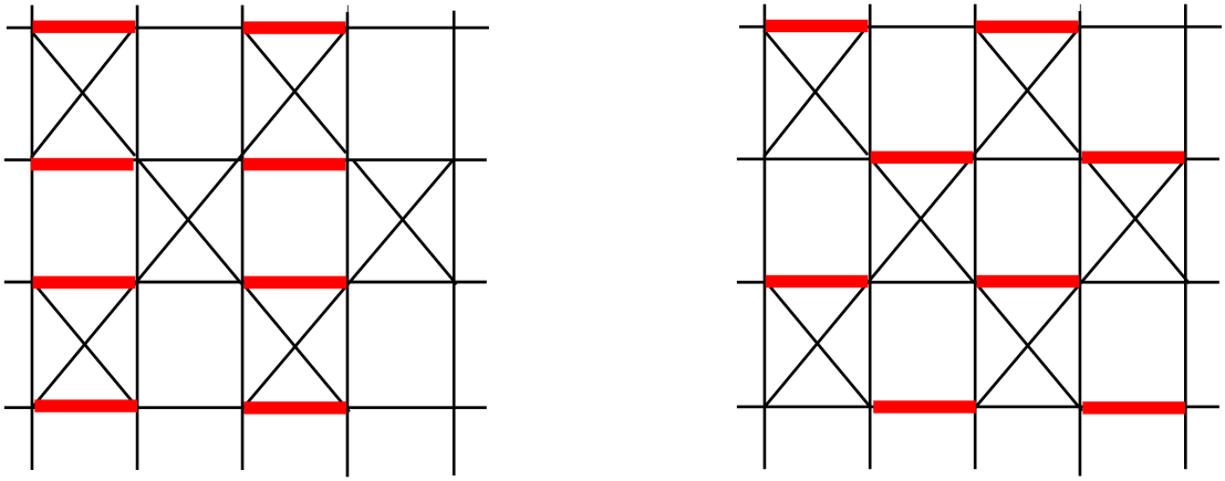
Figure 4.5: Columnar and staggered configuration of dimers (fat links) on the checkerboard lattice: such symmetry breaking configurations are 4-fold degenerate in the thermodynamic limit.

The simplest Valence Bond Crystals that allow the above-mentioned symmetry breaking are described by pure product wave-functions of 4-spin S=0 plaquettes.

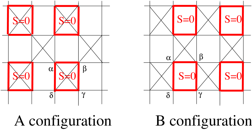
Figure 4.6: S=0 4-spin plaquette valence-bond crystals on the checkerboard lattice: fat links indicate 4 spins involved in a singlet.

This family includes eight different configurations:

• The singlet plaquettes may sit either on the squares with crossed links or on the void squares (A and B configurations of Fig. 4.6),

• The translation symmetry breaking configurations may be in two different locations named $A_{1(2)}$ (resp $B_{1(2)}$),

• An S=0 state on a plaquette of four spins sitting on sites ($\alpha,\beta,\gamma,\delta$) may be realized either by the symmetric combination of pairs of singlets:

  $$|\psi^{+}>=|\alpha\to\delta>|\gamma\to\beta>+|\alpha\to\beta>|\gamma\to\delta>,$$ (4.3)

  or by the anti-symmetric one:

  $$|\psi^{-}>=|\alpha\to\delta>|\gamma\to\beta>-|\alpha\to\beta>|\gamma\to\delta>.$$ (4.4)

  where $|\alpha\to\gamma>$ is the singlet state on sites $\alpha$ and $\gamma$:

  $$|\alpha\to\gamma>=(|\alpha\uparrow,\gamma\downarrow>-|\alpha\downarrow,\gamma\uparrow>)/\sqrt{2}.$$ (4.5)

Wave-function	${\cal T}_{{\bf u}_{1}}$	${\cal R}_{\pi/2}$	${\cal\sigma}_{{\bf u}_{1}}$
$A_{1(2)}^{+}$	$A_{2(1)}^{+}$	$A_{1(2)}^{+}$	$A_{1(2)}^{+}$
$A_{1(2)}^{-}$	$A_{2(1)}^{-}$	$(-1)^{p}A_{1(2)}^{-}$	$(-1)^{p}A_{1(2)}^{-}$
$B_{1(2)}^{+}$	$B_{2(1)}^{+}$	$B_{2(1)}^{+}$	$B_{2(1)}^{+}$
$B_{1(2)}^{-}$	$B_{2(1)}^{-}$	$(-1)^{p}B_{2(1)}^{-}$	$(-1)^{p}B_{2(1)}^{-}$
$X^{\eta}=A_{1}^{+}+\,\eta\,A_{2}^{+}$	$\eta\,X^{\eta}$	$X^{\eta}$	$X^{\eta}$
$Y^{\eta}=A_{1}^{-}+\,\eta\,A_{2}^{-}$	$\eta\,Y^{\eta}$	$(-1)^{p}Y^{\eta}$	$(-1)^{p}Y^{\eta}$
$Z^{\eta}=B_{1}^{+}+\,\eta\,B_{2}^{+}$	$\eta\,Z^{\eta}$	$\eta\,Z^{\eta}$	$\eta\,Z^{\eta}$
$T^{\eta}=B_{1}^{-}+\,\eta\,B_{2}^{-}$	$\eta\,T^{\eta}$	$(-)^{p}\,\eta\,T^{\eta}$	$(-)^{p}\,\eta\,T^{\eta}$

Table 4.1: Transformation rules of the product wave-functions in the elementary operations of the symmetry group (the space group is defined with respect to point O and translations ${\bf u_{1},u_{2}}$). The wave-functions of the anti-symmetric plaquettes have different symmetries depending on the parity p of the number of plaquettes in the sample.

We can thus define eight different product wave-functions labeled: $|A_{1(2)}^{\epsilon}>$ and $|B_{1(2)}^{\epsilon}>$. The transformations of these states under the elementary operations of the lattice symmetry group are described in the first four lines of Table 4.1. The symmetric (resp. anti-symmetric) linear combinations of these states which are irreducible representations of this group are defined in the four last lines of the same Table. Comparison of the symmetries of these states for different samples with those of the two first levels of the exact spectra indicates a $Z^{+},Z^{-}$ symmetry of the HCKB ground-state doublet. In the thermodynamic limit the symmetry breaking configuration is thus of the B type decorated by the symmetric 4-spin plaquettes $|\psi^{+}>$ described in Eq. 4.3.

A simple last remark could be done: the symmetric-plaquette state (Eq. 4.3) can be rewritten as the product of two triplets along the diagonals of the square. This configuration of spins is not energetically optimal on the squares with antiferromagnetic crossed links (A configuration) but might a priori be favored in B configuration. Reversely the $\psi^{-}$-plaquette can be rewritten as the product of two singlets along the diagonals of the square, and would eventually be preferred in A configuration. The variational energy per spin of the product wave-function of $\psi^{+}$-plaquettes in B configuration is $E_{var}(B^{+})=-0.5$, whereas the variational energy per spin of the product wave-function of $\psi^{-}$-plaquettes in A configuration is $E_{var}(A^{-})=-0.375$. The exact energy per spin is $E_{ex}\sim-0.514\pm 0.006$. This is a first proof that the real system takes advantage of some fluctuations around the pure product wave-function $Z^{+}$ to decrease its energy.

The study of dimer-dimer correlations (Fig. 4.7 and Table 4.2):

$${\cal C}^{4}(1,2;i,j)=4\left[<{\bf S}_{1}.{\bf S}_{2}\;{\bf S}_{i}.{\bf S}_{j}>-<{\bf S}_{1}.{\bf S}_{2}><{\bf S}_{i}.{\bf S}_{j}>\right]$$ (4.6)

and 8-spin correlation functions [fmsl03] shows long range order in the 4-spin plaquettes, but also the dressing of the pure product state $Z^{+}$ by quantum fluctuations (see Table 4.2).

Are those small size computations relevant for the description of the thermodynamic limit? The stronger answer is read in Fig. 4.3 $\&$ Fig. 4.4: insofar as the degeneracy of the ground-state and the gaps to the first triplet state and the third singlet state remain finite in the thermodynamic limit, the Valence Bond Crystal picture (with LRO in plaquettes) will survive to quantum fluctuations. The gaps results (Fig. 4.3 $\&$ Fig. 4.4) show that the studied samples (except the $N=16$) have linear sizes of the order of, or larger than the spin-spin correlation length. We thus think that the present qualitative conclusions are reliable.

${i,j}$	ex. g.-s.	Z w-f.	${i,j}$	ex. g.-s.	Z w-f.
31,32	.56	.63	7,13	.10	.25
7,8	.43	.42	19,25	.10	.25
25,26	.26	.25	7,12	-.10	-.25
13,14	.26	.25	31,36	-.10	-.25
19,20	.25	.25	13,18	-.11	-.25
6,5	.22	.25	25,30	-.11	-.25
6,12	-.20	-.25	19,24	-.11	-.25
25,31	-.20	-.25	6,36	.10	.25
13,19	-.18	-.25	12,18	.11	.25
36,35	.18	.25	24,30	.10	.25
5,11	-.18	-.25	35,5	.10	.25
4,10	-.18	-.25	11,17	.10	.25
12,11	.17	.25	29,23	.10	.25
36,30	-.15	-.25	5,4	-.11	-.25
35,29	-.15	-.25	11,10	-.11	-.25
30,29	.15	.25	35,34	-.11	-.25
17,23	-.15	-.25	17,16	-.11	-.25
18,17	.15	.25	29,28	-.10	-.25
18,24	-.15	-.25	23,22	-.10	-.25
24,23	.15	.25	34,4	.10	.25
28,34	-.15	-.25	10,16	.10	.25
16,22	-.15	-.25	28,22	.10	.25

Table 4.2: Dimer-dimer correlations ${\cal C}^{4}(1,2;i,j)$ (Eq. 4.6) in the $N=36$ ground-state. The sites $1,2,i,j$ are described in Fig. 4.7, the $i,j$ points are enumerated in the first columns. This correlation has been measured in the exact ground-state wave function (second columns) and in the variational Z state (third columns). All the values of these correlations between sites of Fig. 4.7 can be obtained from this table by a mirror symmetry through the bisector of bond $(1,2)$.

Figure 4.7: Dimer-dimer correlations in the exact ground-state of the 36 sample (Eq. 4.6). The reference bond is the bond $(1,2)$. Positive (negative) correlations are drawn as full (dashed) lines. The thickness of the lines is a measure of the strength of the correlation. The diagonal lines show the position of the crossed links.

4.2.4 Excitations: raw data and qualitative description of the first excitations

Looking to Table 4.3 and Fig. 4.8, it appears that the triplet excitations are gapped (gap of the order of 0.7) and very weakly dispersive. Singlet excitations too are gapped (4th line of Table 4.3 and Fig. 4.9); they are much more dispersive than the triplet excitations and less energetic (gap of the order of 0.25).

$N$	24’	28	32*	32’	36
$e_{0}$	-.522	-.520	-.517	-.514	-.520
$E^{1}_{S=1}-E^{1}_{S=0}$	0.58	0.57	0.69	0.57	0.71
$E^{2}_{S=0}-E^{1}_{S=0}$	0.08	0.09	0.03	0.01	0.05
$E^{3}_{S=0}-E^{2}_{S=0}$	0.06	0.05	0.18	0.13	0.22
$E^{1}_{S=1}-E^{3}_{S=0}$	0.44	0.42	0.47	0.43	0.44
$n_{1}$	51	82	286	135	110
$ln(n_{1})$/N	0.16	0.16	0.18	0.15	0.13

Table 4.3: Spectrum of the Heisenberg model on the checker-board lattice. Energy per spin in the ground-state $e_{0}$ and energy gaps $E^{n_{S}}_{S}-E^{n_{S}^{\prime}}_{S^{\prime}}$ between the ${n_{S}^{\prime}}$ energy level of the $S^{\prime}$ spin sector and the ${n_{S}}$ level of the $S$ sector. Second line: spin gap. Third line: gap between the absolute ground-state and the first singlet excitation . Fourth line: gap between the second and third level in the $S=0$ sector. Fifth line: gap between the third level in the $S=0$ sector and the first triplet excitation. Following lines: $n_{1}$ is the number of singlet states in the spin gap (including degeneracies). The starred column corresponds to a sample which has the extra symmetries of the pyrochlore lattice.

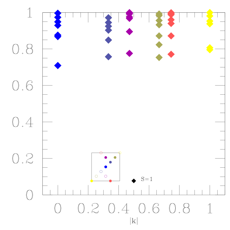
Figure 4.8: Dispersion relations in the triplet sector versus $|{\bf k}|/|{\bf k}_{0}|$ with ${\bf k}_{0}=(\pi,\pi)$.

The inset shows the correspondence between the colors of the symbols and the wave vectors in the Brillouin zone. Only the triplet excitations are drawn in this figure.

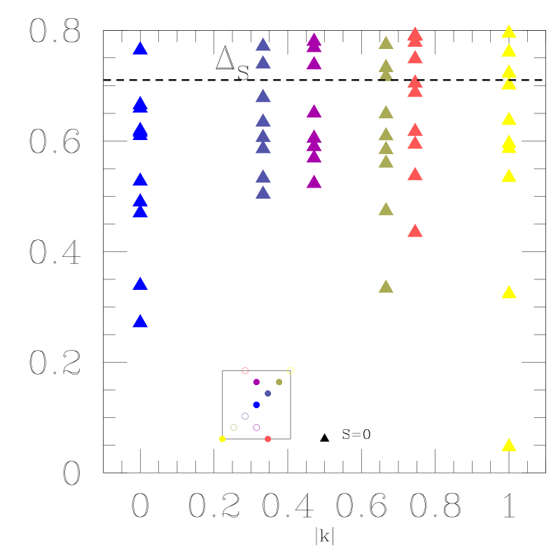
Figure 4.9: Dispersion relation of the singlet excitations of the $N=36$ sample versus $|{\bf k}|/|{\bf k}_{0}|$ with ${\bf k}_{0}=(\pi,\pi)$. The horizontal dashed line indicates the spin-gap.The inset shows the correspondence between the colors of the symbols and the wave vectors in the Brillouin zone. Only the singlet excitations are drawn in this figure. The first excited level of this figure with ${\bf k}_{0}=(\pi,\pi)$ (yellow up triangle) is not a true excitation. This level is at the thermodynamic limit degenerate with the ground-state and allows the space symmetry breaking of the 4-spin plaquette order.

There is a very simple variational description of the triplet excitations: let us consider the 4-spin plaquettes B of the ground-state. The S=0 ground-state is formed from the coupling of two triplets along the diagonals. There are four S=1 states on such a plaquette. The lowest S=1 excitation simply results from the S=1 coupling of the two diagonal triplets. The gap to this variational excitation is 1. The Bloch waves built on such excitations are non dispersive. Up to a renormalization of the gap of the order of $33\%$, this picture appears as a good qualitative description of the true S=1 excitations of the HCKB model, which are massive, quasi localized excitations with an energy gap $\sim 0.7$.

The singlet excitations are more intricate. On a B plaquette the first S=0 excitation corresponds to the antisymmetric coupling of dimers $|\psi^{-}>$ described in Eq. 4.4. Its energy gap to the ground-state is equal to 2. This first excitation of the B plaquettes is more energetic than the object built by a reorganization of two symmetric $\psi^{+}$ states on two neighboring B positions. More precisely the excitation which promotes the two pairs of spins ($\alpha,\delta)$ and ($\beta,\gamma$) into triplet states and then couples them in a singlet states has a gap 1 with respect to the ground-state. To first order in a strong coupling expansion this excitation is non dispersive but it can acquire dispersion at higher order. The exact S=0 excitations are thus certainly a bit more extended and complex that this first approximation.

Remarks on the number of singlet excitations in the singlet-triplet gap

The spectra of very small samples of the HCKB model [52] lead to conclusions on the number of singlets excitations that should be precised and relativized. The above-mentioned authors, and many commentators afterward, argued that this large number of singlets might be reminiscent of the exponential degeneracy in the singlet sector of the Heisenberg model on the kagome lattice. A precise analysis of the spectra of singlet excitations of the HCKB model shows that this analogy is unjustified for the following reasons:

i) The sample set used to extract this conclusion was a mixture of true 2-d checker-board samples, quasi 1-dimensional tubes with a cross section of 4 spins and 3-dimensional pyrochlore-like samples [fmsl03]. Table 4.3 summarizes the results for the restricted family of pure 2-dimensional HCKB samples. Whereas the low density of singlet states of the Heisenberg model on the kagome lattice increases as $1.15^{N}$ with the system size, a similar analysis for the HCKB model gives the value $0.14^{N}$. Changing the ratio of the exponential from a number larger than one to a number smaller than one changes indeed completely the picture! In fact the best fit to describe the number of singlet in the spin-gap is obtained for a power law fit: $N^{\gamma}$ with ${\gamma}=3.96$. If these low excitations can be described as modes one would effectively expect some power law.

ii) Last difference between the HCKB model and the Heisenberg model on the kagome lattice (HK): in the HK model the continuum of singlets is adjacent to the ground-state whereas, in the HCKB model, there is a clear-cut gap in the singlet sector between the ground-state multiplicity and the first singlet excitations.

This simple analysis of the singlet and triplet excitations of the HCKB model supports the idea that the excitations are simple “optical modes” that could be observed in Raman, RPE, ESR or NMR spectra. This structure is certainly highly reminiscent of those of dimerized or spin-Peierls chains, gapped ladders.. A picture consistent with the strong coupling description of the ground-state.

4.2.5 Summary of the generic features of a Valence Bond Crystal

I would like to argue that the main features of Valence Bond Crystals (whatever the dimensionality of space where they are living) are probably:

• A spin gap, no $SU(2)$ symmetry breaking and short range spin-spin correlations,

• Degeneracy in the thermodynamic limit of the $S=0$ ground-state, embedding the spontaneous space symmetry breaking of the phase,

• Long range order in dimer-dimer and/or larger $S=0$ plaquettes, (that can subsist up to finite temperature?)

• Gapped excitations, in the $S=0$ sectors as well as in other $S$ sectors, that can be described as modes, more or less dispersive. A strong coupling analysis of these modes seems a priori valid but the examples worked out up to now, on this model or on the Shastry-Sutherland model [55, 56], show that the departure point of the perturbation theory should be given special consideration.

No experimental evidence exists up to now of a pure Valence Bond Crystal with spontaneous symmetry breaking. But a few 2-dimensional systems with a Valence Bond ground-state have been observed experimentally: CaV₄O₉ [57, 58, 59, 60, 61, 62, 63, 64, 65, 66, 67, 68, 69] and SrCu₂(BO₃)₂ [70, 55, 71, 72, 73, 74, 75, 76, 56, 77, 78]. However, in both cases the ground-state is non-degenerate because the Hamiltonian has an integer spin in the unit cell (4 spins $1/2$) and the dimerization does not break any lattice symmetry. From the theoretical point of view on may argue that the difference between the theoretical VBC described in this chapter and these compounds is akin to the difference between the dimerized phase of the $J_{1}-J_{2}$ model on the chain and the spin Peierls compounds. This is a minor difference and from the experimental point of view the first excitations of all these models can be qualitatively described as “optical modes”. The detailed characteristics of the two-quasi-particle continua could be a bit more different.

4.3 A simple model of VBC with a critical point: the hard core quantum dimer model of Rokhsar and Kivelson on the square lattice

Looking for a model with a resonating valence bond ground-state, Rokhsar and Kivelson introduced in 1988 a quantum hard core model on the square lattice [79]. Their motivation was the description of systems with strongly coupled real-space Cooper pairs. At half filling these next-neighbor Cooper pairs can be seen as next-neighbor dimers. Pauli principle and Coulomb interaction imply that these dimers are hard core dimers. Insofar as the spin gap is large enough, it can be speculated that the manifold of low energy states is spanned by the linearly independent set of nearest neighbor dimer coverings. The dynamics of the low lying singlet excitations of this model are described by the Hamiltonian ${\cal H}_{dimer}$:

$$H_{dimer}=\sum_{\rm Plaquette}\left[-J\left(\left|\begin{picture}(13.0,9.0)(-2.0,2.0)\put(0.0,0.0){\line(0,1){8.0}} \put(8.0,8.0){\line(0,-1){8.0}} \put(0.0,0.0){\circle*{3.0}} \put(0.0,8.0){\circle*{3.0}} \put(8.0,0.0){\circle*{3.0}} \put(8.0,8.0){\circle*{3.0}} \end{picture}\right>\left<\begin{picture}(13.0,9.0)(-2.0,2.0)\put(0.0,0.0){\line(1,0){8.0}} \put(8.0,8.0){\line(-1,0){8.0}} \put(0.0,0.0){\circle*{3.0}} \put(0.0,8.0){\circle*{3.0}} \put(8.0,0.0){\circle*{3.0}} \put(8.0,8.0){\circle*{3.0}} \end{picture}\right|+h.c.\right)+V\left(\left|\begin{picture}(13.0,9.0)(-2.0,2.0)\put(0.0,0.0){\line(0,1){8.0}} \put(8.0,8.0){\line(0,-1){8.0}} \put(0.0,0.0){\circle*{3.0}} \put(0.0,8.0){\circle*{3.0}} \put(8.0,0.0){\circle*{3.0}} \put(8.0,8.0){\circle*{3.0}} \end{picture}\right>\left<\begin{picture}(13.0,9.0)(-2.0,2.0)\put(0.0,0.0){\line(0,1){8.0}} \put(8.0,8.0){\line(0,-1){8.0}} \put(0.0,0.0){\circle*{3.0}} \put(0.0,8.0){\circle*{3.0}} \put(8.0,0.0){\circle*{3.0}} \put(8.0,8.0){\circle*{3.0}} \end{picture}\right|+\left|\begin{picture}(13.0,9.0)(-2.0,2.0)\put(0.0,0.0){\line(1,0){8.0}} \put(8.0,8.0){\line(-1,0){8.0}} \put(0.0,0.0){\circle*{3.0}} \put(0.0,8.0){\circle*{3.0}} \put(8.0,0.0){\circle*{3.0}} \put(8.0,8.0){\circle*{3.0}} \end{picture}\right>\left<\begin{picture}(13.0,9.0)(-2.0,2.0)\put(0.0,0.0){\line(1,0){8.0}} \put(8.0,8.0){\line(-1,0){8.0}} \put(0.0,0.0){\circle*{3.0}} \put(0.0,8.0){\circle*{3.0}} \put(8.0,0.0){\circle*{3.0}} \put(8.0,8.0){\circle*{3.0}} \end{picture}\right|\right)\right]$$ (4.7)

(In their original paper the authors discussed the derivation of this effective Hamiltonian from a more realistic Hubbard model.)

The first term of Eq. 4.7 describes the spatial flip of two parallel dimers from horizontal to vertical position and vice-versa, it could also be seen as a cyclic permutation of the two dimers around a square: it is a kinetic energy term which favors resonances between different configurations of parallel dimers ($J$ is always $>0)$. The second term is a potential energy term likely to be repulsive in the original electron model. The ground-state for infinitely large $\frac{|V|}{J}$ is a Valence Bond Crystal, either staggered (for large $\frac{V}{J}>0$), or columnar (for large $\frac{V}{J}<0$). See Fig. 4.3.

Topological structure of the Hilbert space of the QHCD model on the square lattice

The eigenstates of ${\cal H}_{dimer}$ can be classified according to their winding numbers ($\Omega_{x},\Omega_{y}$) across the 2-torus of the square sample with periodic boundary conditions. There are many equivalent ways to define these winding numbers. Let us follow RK. They draw the transition graph of a dimer configuration ${\cal C}$ relative to a reference configuration ${\cal C}_{0}$ (which may be the columnar configuration) as the superposition of the dimer coverings of the two configurations ${\cal C}$ and ${\cal C}_{0}$. The dimers in ${\cal C}$ are directed from one sublattice to the other and reversely for the dimers of ${\cal C}_{0}$. The transition graph thus appears as a graph of oriented loops. The winding number $\Omega_{x}$ (resp. $\Omega_{y}$) measures the net number of loops (clockwise minus counter-clockwise) encircling the torus in the $x$ (resp $y$ direction). The Hamiltonian does not couple subspaces with different winding numbers. These pairs of winding numbers define $N_{s}$ disconnected topological subspaces (where $N_{s}$ is the number of lattice sites).

For $V\geq J\geq 0$, ${\cal H}_{dimer}$ is positive semi-definite, the ground-state is unique and nodeless (Frobenius theorem). Moreover 0 is a lower bond of its energy.

Demons: A lower bond for the ground-state energy is given by a minimization of the Hamiltonian on each plaquette individually. If the given plaquette has no parallel dimer (non flippable plaquette), its energy is zero and if it has parallel dimers it has a potential energy $V$ and at best a kinetic energy of $-J$. We can thus write a lower bond energy of the global system, which is proportional to the number of flippable plaquettes $n_{flip}$, as $min\left[0,(V-J)n_{flip}\right]$.

Phase Diagram of the RK model

The staggered configuration is a zero-energy eigenstate of ${\cal H}_{dimer}$.

At the point $\frac{V}{J}=1$ the model is exactly solvable.

• The four staggered configurations are zero-energy eigenstates of ${\cal H}_{dimer}$. As they saturate the low energy bond, they are the ground-states for $V\geq J\geq 0$. They can be classified in two different topological classes in which they are the only representatives. They have a zero energy and any configuration of other topological subspaces has a larger strictly positive energy (at least of order ${\cal O}(L)$ in the limit $\frac{V}{J}\to\infty$ ).

• At the point $\frac{V}{J}=1$ the model is exactly solvable. There is in each topological subspace a ground-state with zero energy. It is the equal amplitude superposition of all the configurations of that sector. i) Simple computation shows that these states are zero-energy states of ${\cal H}_{dimer}$. ii) Since all off-diagonal elements are non-positive the ground-state is unique and nodeless (Frobenius property, Marshall theorem). The equal amplitude states are thus the unique ground-states in their respective topological sectors. We will call these states the RK states. This is the first example in these lectures of a Resonating Valence Bond wave-function.

• It has been shown by Kohmoto and Shapir [82], that the spin-spin correlations in this state decrease exponentially.

• An important property: any dimer correlation functions in the RK state can be computed from an exact mapping to the classical statistical problem of dimer coverings first solved by M. E. Fisher and J. Stephenson [83]. From this work one can conclude that the dimer-dimer correlation functions at $\frac{V}{J}=1$, decreases algebraically with distance (as $r^{-2}$). This property implies that the first excitations above the ground-states are gapless.

• On the basis of the continuity in the energy between the staggered phase and the RK states, one may speculate that the RK point is the quantum critical end of the staggered VBC phase. But the excitations of the staggered VBC are non local and have energy of order ${\cal O}(N^{+0.5})$ in the $\frac{V}{J}\to\infty$ limit. To sustain the above point of view one should explain how the kinetic term can dress these excitations so that they become gapless when $\frac{V}{J}\to 1$. In fact the more probable hypothesis is a first order phase transition between the RK phase and the staggered one. Such a question could perhaps be answered with Monte Carlo simulations.

• The ground-state wave-function at this RK point has a property which is considered as constitutive of a RVB spin liquid: that is resonances between all dimer coverings. It must be underlined here that this resonance phenomenon at the RK point does not bring any stabilization of the equal amplitude superposition ground-state when compared to the neighboring staggered VBC phase.

• RK then argue that for $\frac{V}{J}<1$, there is, separated by a first order phase transition, a new phase which might be a “true” resonating Valence Bond Spin Liquid . The characterization of this phase is for the moment rather loose: RK argument is variational and rather week. The first calculation by Sachdev on a 36 lattice [84], gives evidence for a VBC columnar state for $\frac{V}{J}<0.5$ and not a clear conclusion nearer from the RK point. Extending the calculations to 64 sites, and using various estimators, Leung and co-workers [85] estimated that long range columnar order probably exists up to the RK point, with the restriction that up to $\frac{V}{J}\sim-0.2$ the order is very plausibly purely columnar, whereas in the range $-0.2<\frac{V}{J}<1$ the order could reduce to a 4-spin S=0 plaquette order . It seems nevertheless widely admitted [86, 87] that this model has crystalline order everywhere except at the RK critical point.

In view of these results for the QHCD model on the square lattice, of most studies on the $J_{1}-J_{2}$ $SU(2)$ model, and of the $SU(N)$ studies on the same lattice [88, 89], one may be tempted to conclude that VBC is the paradigm of the quantum ground-state on square and possibly bipartite lattices. This might be an escapable assumption [51, 20], but the fact is that the triangular based lattices (see next chapters) seem much more favorable to Resonating Valence Bond Spin Liquids.

Chapter 5 Resonating Valence Bond Spin Liquid (Type I)

The Resonating Valence Bond Spin Liquid is a quantum concept introduced in 1973 by P. W. Anderson [18], following the line of thought of Linus Pauling for molecules. When the semi-classical Néel states or simple dimer covering solutions are very far to satisfy each individual bond, Anderson speculated that the macroscopic system could take advantage of the quantum resonances between the exponential number of dimer coverings to lower its ground-state energy. Such states have no long range order whence the name of Spin Liquid, quantum resonances between the exponential number of equivalent dimer coverings are essential: it is a Resonating Valence Bond Spin Liquid (abbreviated as RVB Spin Liquid or RVBSL in the following).

5.1 Introduction: short range versus long range Resonating Valence Bond wave-functions

Resonating Valence Bond wave-functions encompass a large class of wave-functions beyond the equal amplitude superposition of next neighbor dimer coverings that we encounter at the RK point in the last chapter.

It is easy to verify that the whole set of dimer coverings (without any restriction on the length of the dimers) is an overcomplete basis of the $S=0$ subspace of the spin system (compare the numbers of these coverings to the size of the $S=0$ subspace for a N site lattice) .

Let us suppose that we have designed a family ${\cal E}$ of linearly independent dimer coverings ${\cal C}_{i}$, a general RVB wave-function will be written as:

$$|RVB>=\sum_{{\cal C}_{i}\in{\cal E}}A({\cal C}_{i})|{\cal C}_{i}>$$ (5.1)

where $|{\cal C}_{i}>$ are products of dimer wave-functions (with a sign conventionally fixed, respecting the lattice topology).

In variational calculations, one generally use restricted forms of Eq. 5.1, where the amplitude $A({\cal C}_{i})$ of a given configuration ${\cal C}_{i}$ is written as the product of amplitudes $h(k,l)$ for each dimer $(k,l)$ present in ${\cal C}_{i}$.

Two situations have been studied:

i) either long range RVB wave functions where the function $h(k,l)$ depends algebraically on the distance $r_{kl}$ between sites $k$ and $l$ (at least for large distances):

$$h(k,l)=\frac{Cst}{r_{kl}^{\sigma}}$$ (5.2)

Liang, Douçot et Anderson [90] have shown that such wave functions have Néel long range order in the Heisenberg model on the square lattice if $\sigma<5$ and no Néel long range order for $\sigma>5$ . Capriotti and co-workers [51] have used a $p$-wave BCS wave-function for the $J_{1}-J_{2}$ model on the square lattice, which has no long range order in dimers.

i) or the short range Valence Bond w.-f. where the amplitudes $h(k,l)$ are not necessarily strictly restricted to next neighbors but decrease at least exponentially with distance (most of the following is concerned with that kind of wave functions). By construction such functions cannot describe Néel long range order, as Néel order has long range correlations between spins on the same sublattices. As we have seen in the previous chapter, this family encompasses the quantum critical behavior of the QHCD model on the square lattice. We can equally describe in this basis the Valence Bond Crystals, which are characterized by dominant amplitudes associated to the simple symmetry breaking configurations. Many properties of these wave-functions have been studied theoretically ([91, 92, 93, 80, 81] and references therein), we will see some of them in the following.

In this chapter we will first describe with some length the properties of the QHCD model on the triangular lattice, to compare to the solution of the same model on the square lattice. We will then move to the Multi-Spin Exchange Hamiltonian on the same lattice, which is the first $SU(2)$ model exhibiting a “true” resonating Valence Bond Spin Liquid. A special attention will be given to the topological degeneracy of the ground-state, and to the existence of deconfined spin-1/2 “spinons” excitations, which is the most important experimental signature of a RVB Spin Liquid state. We will close the chapter by a small bibliography on gauge theory approaches that have been dealing with the same physical problem.

5.2 The Quantum Hard Core Dimer model on the triangular lattice

The QHCD model on the triangular lattice has been studied by Moessner and Sondhi in 2001 [87], when they realized that the dimer-dimer correlation function on this lattice was not algebraically decreasing as on the square lattice but exponentially decreasing with distance. The model on the triangular lattice comprises the same ingredients as on the square lattice: a potential energy term between parallel pairs of dimers and a kinetic energy term which does a cyclic permutation of parallel dimers on 4-spin plaquettes (involving two triangular units).

$$H_{dimer}=\sum_{\rm Plaquettes}\left[-J\left(\left|\begin{picture}(19.0,11.0)(-2.0,2.0)\put(0.0,0.0){\line(1,2){5.0}} \put(10.0,0.0){\line(1,2){5.0}} \put(0.0,0.0){\circle*{3.0}} \put(5.0,10.0){\circle*{3.0}} \put(10.0,0.0){\circle*{3.0}} \put(15.0,10.0){\circle*{3.0}} \end{picture}\right>\left<\begin{picture}(19.0,11.0)(-2.0,2.0)\put(0.0,0.0){\line(1,0){10.0}} \put(5.0,10.0){\line(1,0){10.0}} \put(0.0,0.0){\circle*{3.0}} \put(10.0,0.0){\circle*{3.0}} \put(5.0,10.0){\circle*{3.0}} \put(15.0,10.0){\circle*{3.0}} \end{picture}\right|+h.c.\right)+V\left(\left|\begin{picture}(19.0,11.0)(-2.0,2.0)\put(0.0,0.0){\line(1,2){5.0}} \put(10.0,0.0){\line(1,2){5.0}} \put(0.0,0.0){\circle*{3.0}} \put(5.0,10.0){\circle*{3.0}} \put(10.0,0.0){\circle*{3.0}} \put(15.0,10.0){\circle*{3.0}} \end{picture}\right>\left<\begin{picture}(19.0,11.0)(-2.0,2.0)\put(0.0,0.0){\line(1,2){5.0}} \put(10.0,0.0){\line(1,2){5.0}} \put(0.0,0.0){\circle*{3.0}} \put(5.0,10.0){\circle*{3.0}} \put(10.0,0.0){\circle*{3.0}} \put(15.0,10.0){\circle*{3.0}} \end{picture}\right|+\left|\begin{picture}(19.0,11.0)(-2.0,2.0)\put(0.0,0.0){\line(1,0){10.0}} \put(5.0,10.0){\line(1,0){10.0}} \put(0.0,0.0){\circle*{3.0}} \put(10.0,0.0){\circle*{3.0}} \put(5.0,10.0){\circle*{3.0}} \put(15.0,10.0){\circle*{3.0}} \end{picture}\right>\left<\begin{picture}(19.0,11.0)(-2.0,2.0)\put(0.0,0.0){\line(1,0){10.0}} \put(5.0,10.0){\line(1,0){10.0}} \put(0.0,0.0){\circle*{3.0}} \put(10.0,0.0){\circle*{3.0}} \put(5.0,10.0){\circle*{3.0}} \put(15.0,10.0){\circle*{3.0}} \end{picture}\right|\right)\right]$$ (5.3)

The sum over plaquettes runs on the three kinds of plaquettes with orientations at 60 degrees from each other.

J can be assumed to be positive : it enforces resonance effects, V can be positive (repulsion between dimers) or attractive. The conditions of validity are the same as those of the model on the square lattice: it is supposed that the spin gap is large enough so that the first excitations are in the singlet sector. Insofar as the spin gap is large, the spin-spin correlations are short range which is consistent with the restriction to the subspace of nearest-neighbor Valence Bonds.

The properties of the lattice affect the properties of the QHCD model on two central points:

• In the triangular case due to the higher entanglement of the lattice with the two-dimer terms, there is only 4 different topological sectors classified according to the parity of the winding numbers: (even, even), (even, odd), (odd, even), (odd, odd). (The dimer-flip term can change the winding numbers, not their parities).

• At temperature much larger than $J$ and $V$, the square lattice problem has algebraically decreasing dimer-dimer correlations, whereas on the triangular lattice these correlations decrease exponentially [87].

As in the square lattice case, at the point $J=V$ the model is exactly solvable. The ground-states here too are the equal amplitude superpositions of all dimer coverings in each topological sector.

Demons: A lower bond for the ground-state energy is given by a minimization of the Hamiltonian on each plaquette individually. If the given plaquette has no parallel dimer (non flippable plaquette), its energy is zero and if it has parallel dimers its potential energy is $V$ and its kinetic energy is $\leq-J$. We can thus write a lower bond for the energy of the global system, which is proportional to the number of flippable plaquettes $n_{flip}$, as $min\left[0,(V-J)n_{flip}\right]$. At $V=J$ the equal amplitude wave-functions in each topological sub-sector saturate this lower bond. As ${\cal H}_{dimer}$ is positive semi-definite at this point, the equal amplitude wave-functions are thus the unique ground-states of the problem.

Contrary to the case of the square lattice, the degeneracy of this RVB subspace is only 4 on the triangular lattice (whereas it is of order N in the square lattice case). As in the square lattice case, these RVB states are degenerate with the 6 staggered configurations, which are ground-states for any $V/J\geq 1$ (see Fig. 5.1).

The sum over all configurations of the equal amplitude wave-functions is equivalent to the classical dimer problem (up to the question of the staggered phase which has a negligible statistical weight in the problem): thus the dimer-dimer correlations decrease exponentially with distance at the point $J=V$. It’s the description of a true RVB Spin Liquid phase with exponentially decreasing spin-spin and dimer-dimer correlations (we thus expect a gap in the singlet sector), and translational invariance of the ground-state (all four topological ground-states, with equal amplitude wave-functions are in the same ${\bf k}=(0,0)$ sector of the impulsion [81]).

Monte-Carlo simulations [87] have shown that this phase extents at least in the range $2/3<V/J\leq 1$. It terminates at $V/J=1$, with a first order transition to the staggered phase (seen in the Monte Carlo simulations as hysteretic behaviors). The dimer-dimer correlation function is very short range in all the above-mentioned range of parameter, and very weakly dependent on temperature, which is suggestive of a gap in the spectrum.

We will not comment on the rest of the phase diagram, as it is not relevant to our main point here. It is described in Fig. 5.1. (For more details, see the original paper [87]).

Figure 5.1: The phase diagram of the Quantum Hard Core Dimer problem on the triangular lattice

Spinons: As noted above the RVB phase has a gap to collective excitations, which is equally true of VBC. The major difference insofar between VBC and RVB Spin Liquids is the existence in this new quantum phase of deconfined spin-1/2 excitations: the spinons. If you break a Valence Bond in a VBC phase and try to separate the two single spins from each other the energy of the system increases as the length of the string of misaligned dimers which appears between the two single spins (take as an example the staggered or the columnar phase of the QHCD). This creates an elastic restoring force which binds the two spin-1/2 together: in such a Valence Bond Crystals excitations have always an integer spin ($\Delta S=0$ or $1$). We suspect that in the RVB Spin Liquid state, where the correlations between local operators are short range and any disordered configuration as probable as an other, the restoring force between two single spins beyond a certain distance will be negligible and the spin-1/2 (“spinons”) will be deconfined. A simple verification can be done on the equal amplitude states of the Quantum Hard Core Dimer model whatever the lattice: spinons do not interact beyond one lattice step. One expects this property to extend in all the RVBSL phase at T=0. At high temperature the classical square lattice is known to be logarithmically confining [83]. Moessner and Sondhi have checked that the triangular lattice is not confining.

The existence of deconfined spin-1/2 excitations, and thus of a continuum of excitations just above the gap is the main experimental signature of the 2-dimensional Valence Bond Spin Liquid. It was recently claimed that this continuum of excitations has been observed in Cs₂CuCl₄ which is supposed to be a two dimensional magnet [94].

Two more complex evidences of RVB Spin Liquids phases had been obtained before the discovery of this simple toy model: the first in 1992 in a large $N$, $Sp(N)$ analysis of Sachdev [95], the second in a more realistic $SU(2)$ spin model by Misguich and coworkers [96, 97]. This last work will be the object of the next section.

5.3 The MSE model or Ring Exchange model on the triangular lattice

The multiple-spin exchange model (called MSE in the following) was first introduced by Thouless [98] to describe the nuclear magnetism of three-dimensional solid He³ [99] and by Herring [100] for the Wigner crystal. It is an effective Hamiltonian which governs the spin degrees of freedom in a crystal of fermions. The Hamiltonian is a sum of permutations which exchange the spin variables along rings of neighboring sites. It is now largely believed that MSE interactions on the triangular lattice also describe the magnetism of solid He³ mono-layers adsorbed on graphite [101, 96, 102] and that it could be a good description of the two dimensional Wigner crystal of electrons [103]. In He³, exchange terms including up to 6 spins are present [101]. Recent discussions equally concern the strength and importance of the 4-spin exchange term in La₂CuO₄ [104, kk03, lst03, 32].

Here we will only focus on 2- and 4-spin interactions which constitute the minimal MSE model where a short-range RVB ground-state is predicted from exact diagonalizations [97]. The Hamiltonian, which is also called by some authors the Ring Exchange model, reads:

$$H=J_{2}\sum_{\begin{picture}(17.0,10.0)(-2.0,-2.0)\put(0.0,0.0){\line(1,0){12.0}} \put(0.0,0.0){\circle*{5.0}} \put(12.0,0.0){\circle*{5.0}} \end{picture}}P_{ij}+J_{4}\sum_{\begin{picture}(26.0,15.0)(-2.0,-2.0)\put(0.0,0.0){\line(1,0){12.0}} \put(6.0,10.0){\line(1,0){12.0}} \put(0.0,0.0){\line(3,5){6.0}} \put(12.0,0.0){\line(3,5){6.0}} \put(6.0,10.0){\circle*{5.0}} \put(18.0,10.0){\circle*{5.0}} \put(0.0,0.0){\circle*{5.0}} \put(12.0,0.0){\circle*{5.0}} \end{picture}}\left(P_{ijkl}+P_{lkji}\right)$$ (5.4)

The first sum runs over all pairs of nearest neighbors on the triangular lattice and $P_{ij}$ exchanges the spins between the two sites $i$ and $j$. The second sum runs over all the 4-sites plaquettes and $P_{ijkl}$ is a cyclic permutation around the plaquette. The 2-spin exchange is equivalent to the Heisenberg interaction since $P_{ij}=2\vec{S}_{i}\cdot\vec{S}_{j}+1/2$, but the four-spin term contains terms involving 2 and 4 spins and makes the model a highly frustrated one.

The general phase diagram of this model is given in Fig. 5.2.

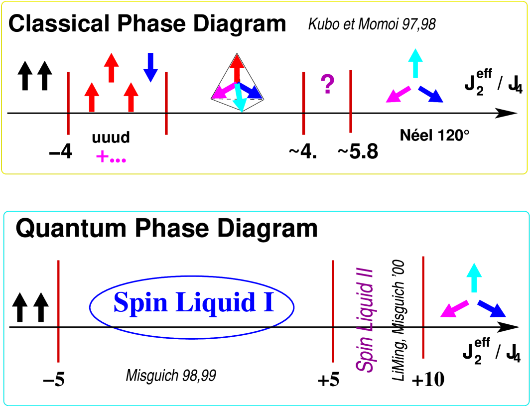
Figure 5.2: The phase diagram of the ring exchange model (Eq. 5.4) on the triangular lattice [107, 97].

We will now focus on the phase described as “Spin Liquid I” in Fig. 5.2 and more precisely on the point $J_{2}<0$ and $J_{2}/J_{4}\simeq-2$ which has been studied extensively by means of exact diagonalizations up to $N=36$ sites [97] (this is a good qualitative description of the low-density solid He³ films).

Finite size effects on the spin gap and energy per spin are displayed in Fig. 5.3.

Figure 5.3: Finite size effects on the spin gap (top graph) and energy per spin (bottom graph) in the Ring Exchange model (Eq. 5.4) for $J_{2}=-2$, $J_{4}=1$. Ref. [97] and unpublished results. Samples with an odd number of sites are indicated by crosses. The full squares are for even samples with the full symmetry of the infinite lattice and open squares for even samples with lower spatial symmetries. Study of the energy per site (bottom figure) is specially interesting. Shape effects are still important for sizes as large as 32 but is appears clearly that the energy of the most frustrated samples (odd number of sites: crosses) is converging to the same limit as the energy of the unfrustrated ones. This is a good indication that the larger sizes that we have considered should allow significant qualitative conclusions.

These data point to a spin-gapped phase with a short correlation length (of the order of a few lattice steps) and a spin gap of order 1.

Three properties should be emphasized:

• No sign of a VBC could be found. All correlations functions spin-spin, dimer-dimer, 4- and 6-spin plaquette-plaquette seem short range [97, 108] and consequently all susceptibilities associated to local observables are zero in the ground-state of the MSE spin liquid (see ref. [81]).

• The ground-state displays at the thermodynamic limit a degeneracy that has been shown to be purely of topological origin [81].

• The system probably supports unconfined spinons .

5.3.1 Topological degeneracy:

This subject is fully developed in ref. [81] and illustrated in Fig. 5.4. In this figure the first graph (top left) shows the low lying singlet states for the N=36 sample. On this graph one sees that these singlet levels appear as multiplets (the black symbol is one time degenerate and the red symbol has a 3-fold degeneracy). With the system size the ”red” levels collapse to the black ones exponentially fast, with a characteristic length which is of the order of $0.6$ lattice step (finite size scaling in the bottom right figure): this is the degeneracy, that we argue to be of topological origin.

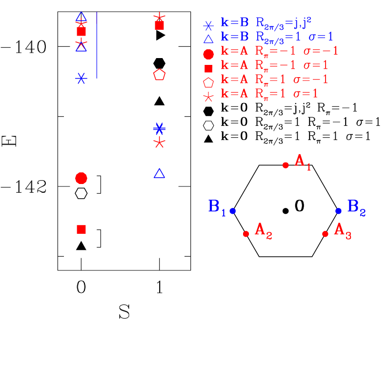
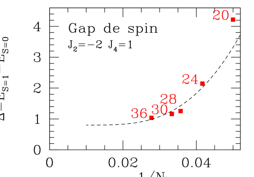
$exp(-L/\xi)$ , $\xi=0.6$.

Figure 5.4: Topological degeneracy in the Ring Exchange model (Eq. 5.4) for $J_{2}=-2$, $J_{4}=1$. Ref. [97] and unpublished results. The figure at the top left shows the low lying levels in the singlet and triplet sectors for the sample of size $N=36$. Notice that the singlet gap is already much smaller than the triplet gap. The figure at the bottom left gives the finite size scaling of the spin gap. The figure at the bottom right shows how the gap in the singlet sector is closing as a function of the size. It is exponentially decreasing with the linear size of the lattice, and the correlation length is about 0.6 lattice step. Such a law correctly describes the finite size scaling of the spin gap of unfrustrated samples (bottom left graph), with an estimate of the spin gap $\sim 0.8\pm 0.1$. The figure in the top right shows the effect of an adiabatic twist of the boundary conditions in exchanging the two quasi-degenerate topological levels.

In short the topological degeneracy can be understood using two arguments: i) the wave-functions describing the MSE spin liquid can be classified as short range RVB wave functions (all the correlations functions in local observables are short range), ii) the Hamiltonian is a local operator insensitive to a global property as the parity of the winding number. In other words for large enough sizes, it is possible to locally optimize the energy and the result does not depend on the topological sector where it is done. As there is 4 topological sectors for a triangular lattice on a two torus, we have there the origin of the 4-fold degeneracy.

On lattices with an odd number of rows it is possible to transform one topological sector in another by a $2\pi$ twist of the boundary conditions along the even direction (Fig 5.4 top-right graph). ( This is equivalent to the introduction of a quantum of fictitious flux through the torus: detailed explanations can be found in ref.[81]). In such an operation the global spectrum of the Hamiltonian is unchanged but eigen-states are not mapped on themselves: the momentum of the states is translated by $(\pi,0)$ in such an operation. Oshikawa [109] concluded that such systems should exhibit a doubling of the Brillouin zone and the spontaneous symmetry breaking of a Valence Bond Crystal. This is an incorrect speculation as we will explain in section 5.5. A simple counter-example is given by the HCQD model: the ground-state in the different topological subspaces for (even, even) samples are all in the ${\bf k}=(0,0)$ sector of the momentum. There is thus an alternation of the quantum numbers of the degenerate ground-state multiplicity when going from (even, even) to (even, odd) samples whatever the system size: this indeed is inconsistent with a VBC spontaneous symmetry breaking in the thermodynamic limit. In the same line, in the MSE model, the evolution with the system size of the quantum numbers associated to the point group equally shows that this topological degeneracy is by no way associated to some symmetry breaking of the lattice [81].

A last comment relative to the possibility of using this degeneracy to produce quantum bits protected from decoherence effects [110, 111]. At first sight the idea is attractive: due to the absence of long range order in any local variable the local susceptibilities vanish in the thermodynamic limit (see ref. [81]) and one expects such quantum bits to be insensitive to any local cause of decoherence. But the charm of this property is to be paid by highly non trivial, if not impossible, writing and reading of the state of the quantum bit (which would imply manipulation of gauge fields ..).

5.3.2 Unconfined spinons?

To estimate the confinement energy of two separated single spins (see Fig.5.5), we use the following arguments:

i) A sample of $2N$ spins has a ground-state energy which is essentially:

$$E(2N,S=0)=2Ne_{\infty}+{\cal O}(\frac{1}{\sqrt{N}}),$$ (5.5)

the correction term to the $N\to\infty$ limit is at most ${\cal O}(\frac{1}{\sqrt{N}})$ if there is long range order in spin-spin correlations and is more plausibly ${\cal O}(\frac{exp(-L/\xi)}{\sqrt{N}})$ in the present case.

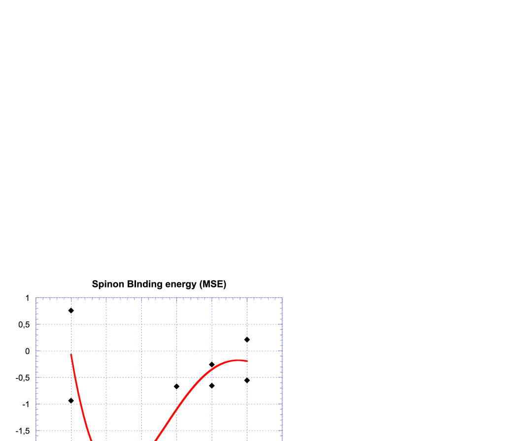
Figure 5.5: Spinons binding energy in the Ring Exchange model (Eq. 5.4) for $J_{2}=-2$, $J_{4}=1$. One sample only has been used for the sizes 28, 29, 30; this precludes an estimation of the uncertainty due to the sample form for intermediate results. Notwithstanding this, the displayed results do not infirm the conclusion of a zero energy binding for large enough sizes. The red curve is an imperfect and arbitrary polynomial fit to indicate a general tendency (unpublished results, work in progress).

ii) A sample withe $2N+1$ sites can accommodate N valence bonds + one single spin, we can write its ground-state energy as:

$$E(2N+1,S=1/2)=(2N+1)\;e_{\infty}+\Delta_{spinon}+{\cal O}(\frac{1}{\sqrt{N}}\cdots)$$ (5.6)

where $\Delta_{spinon}$ measures the energy gap for the creation of one spinon.

iii) If we now look to the first $\Delta S=1$ excitation of an even sample, we expect (in the hypothesis where spinons are the first excitations of this system) that:

$$E(2N,1st\;exc.\;lev.)=2Ne_{\infty}+2\Delta_{spinon}+E_{binding}+{\cal O}(\frac{1}{\sqrt{N}}\cdots)$$ (5.7)

where $E_{binding}$ is the binding energy of two spinons. If $E_{binding}$ is negative in the thermodynamic limit then the spinons will be confined, the first excitations will be integer spin excitations as expected in a Valence Bond Cristal. If $E_{binding}\to 0$ with $\Delta_{spinon}\to\Delta_{0}\neq 0$ with increasing size, we then expect the spinons to be unconfined and the first excitations of the model are fractionalized [112, 113, 114, 115, 116, 117, 118]

Using these three equations (Eqs. 5.5, 5.6, 5.7) for consecutive sizes one obtains an estimate of the binding energy for each sample size. The results are shown in Fig. 5.5. They give a positive indication in favor of unbound spinons in the MSE model.

5.4 RVB Spin Liquids in other spin models

We suspect that RVB Spin Liquids could be observed in other spin models. As already discussed in the previous chapter, the case of the $J_{1}-J_{2}$ model on the square lattice is still debated, the correlation length being probably larger than the largest sizes actually available. The $J_{1}-J_{2}$ model on the hexagonal lattice may have spin liquid phases for $J_{2}/J_{1}\sim 0.3$ and around the point with ferromagnetic $J_{2}$ and $J_{2}/J_{1}=-0.25$ [20]. Here too, and contrary to the MSE model the range of parameters where a spin liquid phase might appear is relatively small, the local S=0 objects probably extend over a few lattice cells, and as a consequence the gaps are rather small and the shape effects a bit chaotic for the available sizes.

An explanation of the robustness of the short-range RVB phase in the MSE model can be guessed from the analogy between multiple-spin interactions and QHCD models. From the analysis of QHCD models we understand that RVB phases are possible when VBC are energetically unstable. Columnar VBC are stabilized by strong parallel dimer attraction and staggered [87] VBC appear when the repulsion between these parallel dimers is strong. In between, an RVB phase can arise . From this point of view, increasing the role of the kinetic term of the model is essential: it is exactly the role of the four-spin ring exchange term of the MSE model (Eq. 5.4)[108].

The role of the triangular lattice (or of a preferred triangular sublattice as in the case of the $J_{1}-J_{2}$ model on the hexagonal lattice) should probably also be emphasized: J.C. Domenge’s preliminary work on the MSE model on the square lattice points to a smaller extent of the Spin Liquid phases [32].

5.5 Short range RVB: topological degeneracy and absence of symmetry breaking

In this section we develop two important properties of type I short range RVB Spin Liquids, in a more general point of view than in the preceding sections and independently of a specific Hamiltonian, with the only restriction that it is a short range operator and that the ground-state and first excited levels can be described with resonant Valence Bond superpositions of short range dimers (not exclusively first neighbors).

(For simplicity this section includes some parts of the paper by Misguich et al.[81] but some demonstrations and examples, which should not alter the general understanding are omitted and in some cases the reader is referred to the original work to complete the picture.)

5.5.1 Topological degeneracy of the ground-state multiplicity of a type I RVB with half integer spin in the unit cell

Definition of the topological sectors

Figure 5.6: 2-torus with one cut $\Delta$.

Let us draw a cut $\Delta$ encircling the torus created by periodic boundary conditions (see Fig. 5.6). This hyper-surface of dimension $d-1$ cuts bonds of the lattice but there is no site sitting on it. The position of the cut is arbitrary. The family of nearest-neighbor dimer coverings can be decomposed into two subspaces ${\cal E}^{\pm}_{\Delta}$ depending on the parity $\Pi_{\Delta}$ of the number of dimers crossing the cut $\Delta$ . By considering a set of $d$ cuts $\Delta_{i=1,\dots,d}$ encircling the torus in all possible directions one obtains $2^{d}$ families of dimer covering.

Any movement of dimers can be represented as a set of closed loops around which dimers are shifted in a cyclic way. A local operator will only generate contractible loops which will cross each cut a even number of times. The number of dimers crossing the cut can therefore only be changed by an even integer and the parities $\Pi_{\Delta_{i}}$ are unchanged.

This property remains true as long as one works in a subspace where the dimer lengths are smaller than the linear system size, that is when the topological sector are well defined (if a dimer length is half the linear of the system one cannot decide by which side it goes). On the other hand, we checked on the triangular (resp. Kagome) lattice that these 4 sectors are the only topological sectors: local 3- (resp 4-) dimer moves can be used to transform a configuration of a given sector into any other configuration of that sector.

These subspaces are orthogonal in the thermodynamic limit [119]. The graph of the scalar product $<c^{+}|c^{-}>$ of two dimer configurations belonging to different subspaces ${\cal E}^{+}$ and ${\cal E}^{-}$ has at least one long loop encircling the torus in the $L_{x}$ direction. When $L_{x}$ goes to infinity this contribution to the scalar product is smaller than $2^{-L_{x}/2}$. Consider two normalized vectors $\left|\Psi^{+}\right>$ and $\left|\Psi^{-}\right>$ belonging to two different sectors:

$$\left|\Psi^{\pm}\right>=\sum_{c^{\pm}\in\mathcal{E}^{\pm}}\Psi^{\pm}(c^{\pm})\left|c^{\pm}\right>$$ (5.8)

Because of the exponential number of dimer coverings in each subspace it is not obvious that $\left|\Psi^{+}\right>$ and $\left|\Psi^{-}\right>$ are orthogonal in the thermodynamic limit. But it is nevertheless the case [81], and:

$$\left<\Psi^{+}|\Psi^{-}\right><{\cal O}(2^{-L/2}).$$ (5.9)

In the following, unless explicitly mentioned, we consider the 2D case for simplicity but most of the topological arguments about dimer covering immediately extend to higher dimensions.

Two-fold degeneracy in even$\times$odd samples

In the special case of tori with an odd number of rows (and an odd number of spin-$\frac{1}{2}$ per crystallographic unit cell), one step translation along the $x$ axis (called ${\cal T}_{x}$ in the following) maps ${\cal E}^{+}$ on ${\cal E}^{-}$ and reversely. Some point-group symmetry can also do this job. A $\pi$ rotation about a lattice site nearby the cut (called ${\cal R}_{\pi}$ in the following) has the same effect. If the cut is chosen parallel to a symmetry axis of the sample, a reflection with respect to this axis (called $\Sigma_{y}$ in the following) will equally map ${\cal E}^{+}$ on ${\cal E}^{-}$ and reversely.

All these symmetry operations isolate a single column $C$ of lattice sites between $\Delta$ and its transform $\Delta^{\prime}$. In that case columns have an odd number of sites and an odd number of dimers must connect some sites inside $C$ with sites outside $C$. Therefore $\Pi_{\Delta}$ differs from $\Pi_{\Delta^{\prime}}$ and the two subspaces ${\cal E}^{+}$ and ${\cal E}^{-}$ are exchanged.

For a large enough system these two sectors are 1) orthogonal, 2) uncoupled by any local Hamiltonian and 3) exchanged by symmetry operations (even$\times$odd). This is enough to insures that they have the same spectrum, irrespectively of the physics of the model, provided it can be described in the short-range dimer space. In fact, quantum numbers of these doublets of degenerate states are fixed by symmetry.

We decompose an eigenstate $|\psi_{0}>$ on the two topological subspaces defined relatively to the cut $\Delta$:

$$\left|\psi_{0}\right>=\left|\psi_{0}^{+}\right>+\left|\psi_{0}^{-}\right>$$ (5.10)

where $\left|\psi_{0}^{\pm}\right>$ belong respectively to the sets ${\cal E}_{\Delta}^{\pm}$. $\left|\psi_{0}\right>$, as an eigenstate of the Hamiltonian with periodic boundary conditions, belongs to an irreducible representation of the translation group. In the following we will also assume an ${\cal R}_{\pi}$ and $\Sigma_{y}$ invariance of the Hamiltonian and that, for simplicity, $|\psi_{0}>$ transforms under a one-dimensional representation under ${\cal R}_{\pi}$ and $\Sigma_{y}$.

$${\cal T}_{x}\left|\psi_{0}\right>=e^{i{\bf k}_{0}\cdot{\bf u}}\left|\psi_{0}\right>$$

$${\cal R}_{\pi}\left|\psi_{0}\right>=\rho^{\pi}_{0}\left|\psi_{0}\right>$$

$$\Sigma^{y}\left|\psi_{0}\right>=\sigma^{y}_{0}\left|\psi_{0}\right>$$ (5.11)

In the thermodynamic limit $\left|\psi_{0}^{+}\right>$ and $\left|\psi_{0}^{-}\right>$ are orthogonal and ${\cal T}_{x}$, ${\cal R}_{\pi}$ and $\Sigma^{y}$ map ${\cal E}^{+}$ on ${\cal E}^{-}$ and reversely:

$${\cal T}_{x}\left|\psi_{0}^{\pm}\right>=e^{i{\bf k}_{0}\cdot{\bf u}}\left|\psi_{0}^{\mp}\right>$$

$${\cal R}_{\pi}\left|\psi_{0}^{\pm}\right>=\rho^{\pi}_{0}\left|\psi_{0}^{\mp}\right>$$

$$\Sigma^{y}\left|\psi_{0}^{\pm}\right>=\sigma^{y}_{0}\left|\psi_{0}^{\mp}\right>.$$ (5.12)

Let us now build the variational state:

$$\left|\psi_{1,\Delta}\right>=\left|\psi_{0}^{+}\right>-\;\left|\psi_{0}^{-}\right>.$$ (5.13)

Eqs. (5.12) imply:

$${\cal T}_{x}\left|\psi_{1,\Delta}\right>=-e^{i{\bf k}_{0}\cdot{\bf u}}\left|\psi_{1,\Delta}\right>$$

$${\cal R}_{\pi}\left|\psi_{1,\Delta}\right>=-\rho^{\pi}_{0}\left|\psi_{1,\Delta}\right>$$

$$\Sigma^{y}\left|\psi_{1,\Delta}\right>=-\sigma^{y}_{0}\left|\psi_{1,\Delta}\right>$$ (5.14)

$\left|\psi_{1,\Delta}\right>$ has thus a wave-vector ${\bf k}_{1}$, a rotation quantum number $\rho_{1}^{\pi}$ and a reflection quantum number $\sigma^{y}_{1}$ related to the quantum numbers of $\left|\psi_{0}\right>$ by the relations:

$${\bf k}_{1}={\bf k}_{0}+(\pi,0)$$

$$\rho^{\pi}_{1}=-\rho^{\pi}_{0}$$

$$\sigma^{y}_{1}=-\sigma^{y}_{0}.$$ (5.15)

It is thus a state orthogonal to the ground-state (even on a finite-size system where the topological sectors are not rigorously orthogonal).

Since any local Hamiltonian has exponentially vanishing matrix elements between different sectors we have

$$\left<\psi_{0}^{+}\right|{\cal H}_{0}\left|\psi_{0}^{-}\right>\to 0$$ (5.16)

and $|\psi_{1,\Delta}>$ is thus degenerate with the absolute ground-state, their symmetries being related by relations (5.15).

Degeneracies in even$\times$even samples

As remarked by Bonesteel [119] on a square lattice a $\pi/2$ rotation exchanges sector $(+,-)$ and sector $(-,+)$ but sectors $(-,-)$ and $(+,+)$ remain inequivalent. A similar phenomenon occurs on the triangular lattice where $2\pi/3$ rotations permute cyclically 3 of the 4 sectors. As a result there are equally in even$\times$even samples exact degeneracies due to these mappings [81]. Readers interested in the details of these degeneracies are referred to the original paper [81].

4-fold degeneracy in RVBSL phases

The numerical data on the type I Spin Liquid phase of the MSE and QHCD models [81] suggest that the ground-state degeneracy is 4 in such a phase whatever may be the shape of the sample.

There is no global mathematical proof of this property but the following physical arguments make it extremely plausible.

Let us make the following assumptions:

a) The ground-state can be described in a short-ranged dimer basis. b) All $n$-dimer correlations ($n=2,3,\cdots$) are short-range and the corresponding correlation lengths are bounded. c) The Hamiltonian is local.

From hypotheses a) and c) it is clear that for a large enough system the four topological sectors are not mixed in the ground-state and the spectrum can be computed separately in each sector. As seen before, we do not have any symmetry operation which connects all four sectors (these operations connect only two or three of the topological subspaces, depending on the geometry of the sample) and we need a physical argument to explain why energies should be the same in each sector (in the thermodynamic limit)?

Because of their topological nature, it is not possible to determine to which sector a dimer configuration belongs by looking only at a finite area of the system. In other words, any dimer configuration defined over a large but finite part of the system can be equally realized in all sectors. The Hilbert space available to the system is the same over any finite region of the system. In the absence of any form of long-range order the system can therefore optimize all its correlations with an arbitrary high accuracy equally well in each sector. At this point we can only conclude that the four sector will have the same energy density and we cannot exclude the existence of a gap between the different topological sectors.

However the numerical results obtained in the QHCD and MSE models indicate that it is not the case and that the four ground-states have asymptotically the same total energy. We think that this should be true for a general short-range RVBSL.

Miscellaneous remarks on the RVB ground-state degeneracy

— Dimers and twist operator. The variational state $\left|\psi_{1,\Delta}\right>$ can be deduced simply from $\left|\psi_{0}\right>$ by changing the sign of the dimers crossing the cut $\Delta$. Such an operation can also been seen as a $2\pi$ twist of the spins of column 0. From the physical point of view the reason why $\left|\psi_{1,\Delta}\right>$ has asymptotically the same energy as $\left|\psi_{0}\right>$ becomes clear: in the absence of stiffness ($\sim$ absence of sensitivity to a boundary twist in the thermodynamic limit) and of long-range spin-spin correlations, the perturbation induced by the boundary condition cannot propagate and does not change the energy of the initial state: its only effect is to change the relative phases of the different topological components of the wave function, and consequently the momentum and space symmetry quantum numbers of the initial state of the even-odd samples.

— Fractionalization and topological degeneracy. To our knowledge all present theoretical descriptions of fractionalized excitations in 2D magnets or related problems [120, 115, 121, 112, 118] (we should also mention topological properties of Laughlin’s wave function for fractional quantum Hall effect [122, 123]) imply topological ground-state degeneracies. In such pictures, the physical operation which transforms a ground-state into another is the virtual creation of a pair of spinons (by dimer breaking) followed by its annihilation after the circulation of one of them around the torus. In such a process a $\pi$ phase-shift is introduced between the topological sectors (as in the above recipe). For samples with an odd number of rows this operation connects eigenstates with different ${\bf k}$ vectors (and space quantum numbers) as described in Eqs. (5.15).

— Numerical studies with a different topology. An interesting check of the pure topological nature of this degeneracy could be obtained by studying the problem no more on a torus but on a surface with a different genus. On a sphere we expect an absence of degeneracy. Unfortunately if a lattice can be represented on an infinite plane, both the number of links $L$ and plaquettes $P$ depend linearly on the number of sites $N$ and Euler’s relation $P-L+N=2-G$ constrains the genius $G$ to be 2 ! The torus is the only possible topology if we require a full translation invariance in both directions. In a recent work, Ioffe et al. [111] have studied the absence of sensitivity to disorder as an evidence for topological phenomenon in the liquid phase of the QHCD model on the triangular lattice. They also used open boundary conditions to modify the topology of the system and argue in that case that the low-energy spectrum is free of edge states which could hide the actual ground-state degeneracy.

— Example of RVB phase with 2 spins in the unit cell. A spin liquid state, seeming very similar to the state observed in the MSE model on the triangular lattice, has been observed in the $J_{1}-J_{2}$ model on the hexagonal lattice [20] for $J_{1}=-1,\;J_{2}=0.3$. No quasi-degeneracy of the ground-state has been noticed. It should be remarked that in this system there are 2 spins $\frac{1}{2}$ per crystallographic unit cell and no degeneracy is expected on the basis of the topological arguments.

5.5.2 Symmetry breaking in gapped phases

From the mathematical point of view, ground-state wave functions that break one-step translations or space group symmetries can be built from linear combinations of the degenerate ground-states of the even-odd samples. In a completely equivalent way, ground-state wave functions that break rotation symmetry can be built in even$\times$even samples. One could thus superficially conclude that spontaneous symmetry breaking is possible in RVBSL, we will show below that this assumption is false.

There are many features which show that this degeneracy property is a subtle one, both from the mathematical and physical viewpoints.

The possible alternation of the spatial properties of the low-lying excitations with the parity of the number of rows of the sample (as observed in the QHCD model on the triangular lattice) is a first difficulty. The degeneracy of the RVBSL is in fact quite different from that appearing in a VBC. We do not expect the VBC ground-state degeneracy to depend on the genus of the sample, as the RVBSL does.

From the physical point of view also the two situations are quite different. An infinitesimal symmetry breaking perturbation is able to select one symmetry breaking ground-state of the VBC, but as we will show below this is impossible in the RVBSL.

Let us call ${\cal A}$ the extensive non-diagonal observable appearing in the VBC in the thermodynamic limit. On a columnar VBC modulated in the u direction, this observable is:

$${\cal A}=\sum_{j=1}^{N}e^{{i{\bf K}_{1}}\cdot{\bf r}_{j}}P_{S=0}({\bf r}_{j},{\bf r}_{j}+{\bf u})$$ (5.17)

where $P_{S=0}({\bf r}_{j},{\bf r}_{j}+{\bf u})$ is the projector on the singlet state of two neighboring spins. ${\cal A}$ connects eigen-states with wave-vector ${\bf k}_{0}$ to states with wave-vector ${\bf k}_{0}+{\bf K}_{1}$ .

On a finite size sample, with periodic boundary conditions, the expectation value of ${\cal A}$ is zero in any eigenstate, but $<{\cal A}^{2}>$ could be non zero. If the order parameter ${\cal P}$ defined by:

$${\cal P}^{2}=<\psi_{g.s.}|{\cal A}^{\dagger}{\cal A}|\psi_{g.s.}>/N^{2}$$ (5.18)

does not vanish in the thermodynamic limit, the system has columnar dimer long range order with wave vector ${{\bf K}_{1}}$.

Let us now consider a perturbation of the Hamiltonian:

$$H_{\delta}=H_{0}-\left(\delta{\cal A}+h.c.\right).$$ (5.19)

At T=0, the intensive linear response on the observable ${\cal A}$ is measured by the susceptibility:

$$\chi=\frac{2}{N}<\psi_{g.s.}|{\cal A}^{\dagger}\frac{1}{H_{0}-E_{g.s}}{\cal A}|\psi_{g.s.}>$$ (5.20)

This susceptibility is bounded from below[124]:

$$\frac{4{\cal P}^{4}N^{2}}{f}<\chi$$ (5.21)

where $f$ is the oscillator strength:

$$f=\frac{1}{N}\left<\psi_{g.s.}|\left[{\cal A},\left[H_{0},{\cal A}\right]\right]|\psi_{g.s.}\right>$$ (5.22)

The demonstration uses the properties of the spectral decomposition associated to the operator ${\cal A}$:

$$S(\omega)=\frac{1}{N}\sum_{n\neq 0}\left|<\psi_{g.s.}|{\cal A}|n>\right|^{2}\delta(\omega-\omega_{n})$$ (5.23)

where $\omega_{n}=E_{n}-E_{g.s}$

$${\cal P}^{2}=\frac{1}{N}\int S(\omega)d\omega$$ (5.24)

Using the Cauchy Schwartz inequality one obtains:

$${\cal P}^{4}\leq\frac{1}{N^{2}}\int\omega S(\omega)d\omega\int\omega^{-1}S(\omega)d\omega$$ (5.25)

where

$$\int\omega S(\omega)d\omega=f/2$$ (5.26)

$$\int\omega^{-1}S(\omega)d\omega=\chi/2$$ (5.27)

which proves inequality (5.21). For a short range Hamiltonian the oscillator strength $f$ is ${\cal O}(1)$ and inequality (5.21) implies that the T=0 susceptibility associated to a finite order parameter diverges at least as the square of the sample size: any infinitesimal symmetry breaking perturbation will select a symmetry breaking state.

We will now show that for a RVBSL, where all the correlations functions are short-ranged with correlation lengths bounded by $\xi$, the susceptibilities of the medium remain finite in the thermodynamic limit. To do so we distinguish in Eq. 5.20 the contributions from the quasi-degenerate states of the topological multiplet (called $|\alpha_{i}>$) from the contribution of the other states of the spectrum, above the physical gap $\Delta$. We thus obtain the following upper bound for the susceptibility:

$$\chi\; = \chi_{\rm top}\;+\chi_{\Delta}$$ (5.28)

$$\chi_{\rm top}\; = \frac{2}{N}<\psi_{g.s.}|{\cal A}^{\dagger}\frac{|\alpha_{1}><\alpha_{1}|}{E_{\alpha_{1}}-E_{g.s.}}{\cal A}|\psi_{g.s.}>$$ (5.29)

$$\chi_{\Delta} \leq \frac{2}{N\Delta}\left[<\psi_{g.s.}|{\cal A}^{\dagger}{\cal A}\right.|\psi_{g.s.}>$$ (5.30)

$$- <\psi_{g.s.}|{\cal A}^{\dagger}|\alpha_{1}><\alpha_{1}|{\cal A}|\psi_{g.s.}>]$$

where $|\alpha_{1}>$ stands for the state(s) of the topological multiplet connected to the absolute ground-state by ${\cal A}$. Using the local properties of ${\cal A}$, ${\cal A}^{\dagger}|\alpha_{1}>$ is in the same topological sector as $|\alpha_{1}>$ and $<\psi_{g.s.}|{\cal A}^{\dagger}|\alpha_{1}>$ is at most of ${\cal O}(N\times 2^{-L/2})$ (see paragraph 5.5.1). As $E_{\alpha_{1}}-E_{g.s.}$ is supposed to decrease as $exp(-L/\xi)$ (see Fig. 5.4) $\chi_{\rm top}$ goes to a constant when the size of the sample goes to infinity, provided $\xi$ is small enough . In a system with exponentially decreasing correlations, ${\cal P}^{2}$ decreases as $1/N$ and $\chi_{\Delta}$ is trivially constant at the thermodynamic limit.

In such a phase an infinitesimal field cannot induce a symmetry breaking and there could not be any spontaneous symmetry breaking.

5.6 Other approaches of type I RVB Spin Liquids

As already said, Sachdev in a large $N$, $Sp(N)$ analysis of the Heisenberg model on the triangular lattice equally found in the extreme quantum case an RVB ground-state and deconfined spinons [95].

An interesting mapping of the dimer models on Ising model in transverse field has been studied by many authors (See refs. [125, 118] and references therein). This approach is one of the ways to give evidence of the parentage between this RVB spin liquid with its fractionalized excitations and the deconfining Ising Gauge theories [126, 127, 128, 118, 116]

5.7 Summary of the properties of type I RVB Spin liquids

To conclude let us summarize the properties of a type I RVB Spin liquid:

• It is a phase which does not break either SU(2) symmetry nor any spatial symmetries of the lattice. Its ground-state is unique up to a topological degeneracy which exists only in systems with an odd number of spin-1/2 in the unit cell, living on a 2-torus (more generally the degeneracy is $2^{g}$, with $g$ the genus of the torus). In that sense it is awkward to call such a phase a disordered phase! None of the classical ideas associated to disorder are relevant to understand the properties of this RVB Spin Liquid phase. If we have to compare it to a liquid phase it is more the superfluid phase of ${}^{4}He$ that we should have in mind!

• All correlation functions in local observables have only short range order, and consequently the susceptibility associated to any local observable is zero a T=0.

• This phase has a gap for all excitations, either in the singlet or the triplet sectors and it supports fractionalized excitations (the “spinons”). The first excitations in the singlet sector correspond in the gauge theory language to the bosons of the gauge field that Senthil and M. P. A. Fisher call ”visons” [127, 128]. Due to the properties of the excitations we expect them to form continua in the spin sectors. The neutron experiment of Coldea and co-workers on Cs₂CuCl₄ is perhaps the first experimental proof of such a state [94].

• An RVB spin liquid state is expected in presence of competing and frustrating interactions. The bandwidth in which this phenomenon can be observed is strongly reduced with respect to the original couplings and often only a small fraction of the original couplings: the case of the MSE system at $J1=-2$ and $J_{4}=1$ (the point where all the results given here have been calculated) is in some sense rather exceptional, as at this point the spin gap is almost as large as the cyclic 4-spin exchange.

Chapter 6 Resonating Valence Bond Spin Liquid (Type II)

Type I RVBSL have a gap in the singlet sector. In the Ising gauge theory approach this gap is essential for the consistency of the theory [128]. The Ising gauge field quasi particles called visons by Senthil and co-workers are vortices of the gauge field, they carry a $Z_{2}$ gauge flux, no spin and have long range interaction with spinons. If the spectrum of these particles has a gap then the spinons are unconfined and the phase is “fractionalized”. If they condense, the long range interaction between them and the spinons frustrate the motions of the latter which remained confined. The gap in the singlet sector (above the topological degeneracy) is a crucial ingredient of Type I RVBSL: as we have learned in the previous chapter it is a property of the MSE Hamiltonian near the ferromagnetic phase.

As displayed in Fig. 5.2, the MSE Hamiltonian near the antiferromagnetic three sublattice Néel order displays a second Spin Liquid phase, with no long range order in any observable, but no gap in the singlet sector [107]. Such a behavior is not a standard Spin Liquid behavior. Could it be a quantum critical behavior similar to that of the Rokhsar Kivelson model at $V=J$? Keeping in mind the restrictions inherent on small size approach of such phenomena, we nevertheless think that the observed phenomenon is distinct from the critical RK behavior on the square lattice (see below). In view of the similarities between the phase seen in the MSE model and the phase observed in the Heisenberg model on the kagome lattice, I took the step to describe the physics that can be observed at that point as something different: a RVB Spin liquid of type II.

In fact as most of the studies done in many groups have been devoted to the Heisenberg model on the kagome lattice (noted HK model in the following), it is on this last model that we will center this last chapter.

6.1 Miscellaneous models on the kagome lattice

There has been a large number of studies devoted to different antiferromagnetic models on the kagome lattice, which is a 2-dimensional lattice of corner sharing triangles (Fig. 6.1).

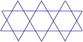
Figure 6.1: The kagome lattice: a lattice of corner sharing triangles. In Japanese kagome is a common word which designs both a basket and the special canwork for baskets. This is equally a trademark for a popular tomato sauce.

The next neighbor Ising model on such a lattice is disordered, its entropy is very large $S_{kag}^{Ising}=0.502$, more than half the independent spin value, much larger than the triangular lattice value $S_{tri}^{Ising}=0.323$ and of the order of Pauling approximation for independent triangles $S_{Pauling}=0.501$ [129]. This suggests that the correlations in this system are very weak: the model remains disordered at all temperatures [130, 131].

Moessner and Sondhi have studied this Ising model in a transverse magnetic field (the simplest way to include in the model some quantum fluctuations): the model fails to order for any transverse field, at any temperature [132, 125].

The n.n. classical Heisenberg model on the kagome lattice has also an extensive T=0 entropy: this is a property easily understood, shared with the same model on different lattices with corner sharing units as the checker-board lattice or the true three dimensional pyrochlore lattice. On all these lattices the n.n. Heisenberg Hamiltonian can be rewritten as the sum of the square of the total spin $S_{\alpha}$ of individual units $\alpha$ (a tetrahedron in the 2-d and 3-d pyrochlore cases and a triangle for the kagome lattice), which share only one vertex. Classical ground-states are obtained whenever $\forall\alpha\;{\bf S}_{\alpha}=0$. This condition fixes the relative position of the three classical spins of a triangle at $120$ degrees from each other in a plane. But it does not fix the relative orientation of the plane of a triad with respect to the planes of triads on corner sharing triangles: the model has thus an infinite local degeneracy and an extensive entropy [133, 131]. This state too is reluctant to order: nevertheless thermal fluctuations select coplanar configurations [133, 131, 134], without long range order in the plane. The order parameter of such a phase is the direction of the local helicity (sometimes called vectorial chirality) and defined by its components as:

$${\zeta}^{\gamma}=\sum_{on\;a\;triangle}\epsilon^{\alpha\beta\gamma}S^{\alpha}_{i}S^{\beta}_{j}$$ (6.1)

where $\epsilon^{\alpha\beta\gamma}$ is the antisymmetric tensor. This kind of order is by analogy to liquid crystals sometimes called a nematic order. The existence of such an order parameter is probably not without relation with the instability of the classical Heisenberg model on the kagome lattice to Dzyaloshinsky-Moriya interactions[135, 136].

6.2 The next-neighbor spin-1/2 Heisenberg model on the kagome lattice: an extreme play-ground for “quantum fluctuations”

The n.n. spin-1/2 quantum Heisenberg model on the kagome lattice has equally been the object of many studies [137, 138, 95, 139, 140, 141, 23, 142, 143, 144]. From these studies one can remember the following facts:

6.2.1 Ground-state energy per spin

The Heisenberg model on the kagome lattice has an extremely low energy per bond ($<{\bf S}_{i}.{\bf S}_{j}>_{per\,bond}=-.437)$ $\sim 87\%$ of the energy per bond of independent triangles. On this lattice the energy per bond of the spin-1/2 system is much lower than the classical energy $\frac{E_{qu.}}{E_{cl.}}\sim 1.74$, a ratio much larger than in any other 2-dimensional magnet, that can only be compared to the value obtained for the Bethe chain (1.77) (see Table. 1.1). The kagome lattice is the 2-dimensional lattice which offers the larger stabilization due to quantum fluctuations.

6.2.2 Correlations

Spin-spin correlations [139], dimer-dimer correlations (Fig. 6.2), chirality-chirality correlations [138] are short range, which is consistent with the previous point.

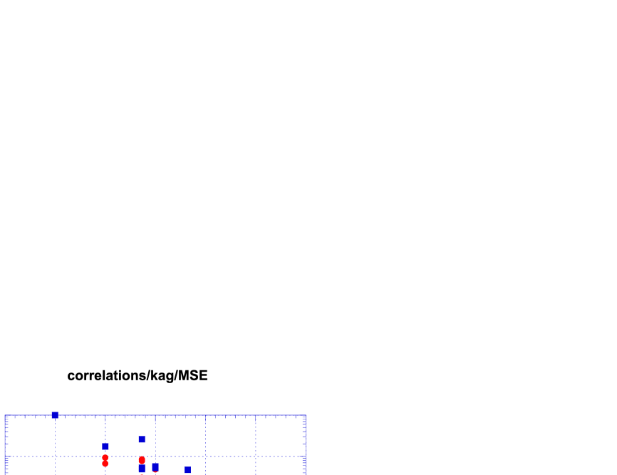
Figure 6.2: Dimer-dimer correlations in the ground-state of the kagome Heisenberg model (blue squares) and in the MSE model (red bullets) versus distance. Although the decrease of these correlations is weaker in the KH model than in the MSE model, it is nevertheless roughly exponential in these first two decades, as the spin-spin correlations are [138, 139]

6.2.3 Spin-gap and absence of gap in the singlet subspace

There is probably a spin-gap of the order of 1/20th of the coupling constant [23]. In view of the smallness of this spin-gap with regards to the available sizes caution is necessary. The above conclusion was drawn from the raw data of exact spectra of samples with up to 36 spins (see Fig. 6.6): more precisely from the measurement of $E_{0}(S=S_{min}+1)-E_{0}(S=S_{min})$, where $E_{0}(S)$ is the lowest energy in the $S$ sector, and $S_{min}=$ 0 or 1/2 depending on the parity of the number of spins of the sample. The size effects on these results are an order of magnitude smaller than in an ordered Néel antiferromagnet. Nevertheless they are still not negligible for these sizes. We have thus tried an indirect measurement of the spin-gap along the following line.

The lowest exact eigenstates in each $S$ sector of a sample of N sites define the energy per spin of the sample at $T=0$ as a function of its magnetization $m=S/(N/2)$. For low value of the magnetization one can fit this energy per spin to an analytic law of the form :

$$e(m)=e(0)+am+bm^{2}/2+{\cal O}(m^{3})$$ (6.2)

The a and b coefficients depend on N. Their physical significance is clear: a measures half the spin gap and

$$b=\frac{\partial^{2}e}{\partial m^{2}}=\chi^{-1}$$ (6.3)

where $\chi$ is the homogeneous susceptibility of the medium for fields larger than the critical field $H_{c}$ ($H_{c}$ in convenient units is equal to the spin gap).

This indirect determination of the spin gap leads to a strong renormalization of the data far small sizes (explaining the large error bars for small sizes data in Fig. 6.3). On the other hand the $N$ dependence of the renormalized data is now much weaker as can be seen by a comparison of the raw results of [23] and Fig. 6.6, with those of Fig. 6.3. A linear extrapolation versus $1/N$ (which should give a lower bound of the spin-gap) leads to the value $0.06$ for the spin gap (consistent extrapolations give $e_{\infty}=-0.4365$ and $\chi_{\infty}=0.34$). All these determinations are in agreement with the results obtained from the raw data. Nevertheless is should be underlined that even for N=36 at the smallest non zero magnetization the linear term of equation (6.2), is only $90\%$ of the quadratic term: this shows the limit of confidence in our assumption on the existence of a spin-gap .

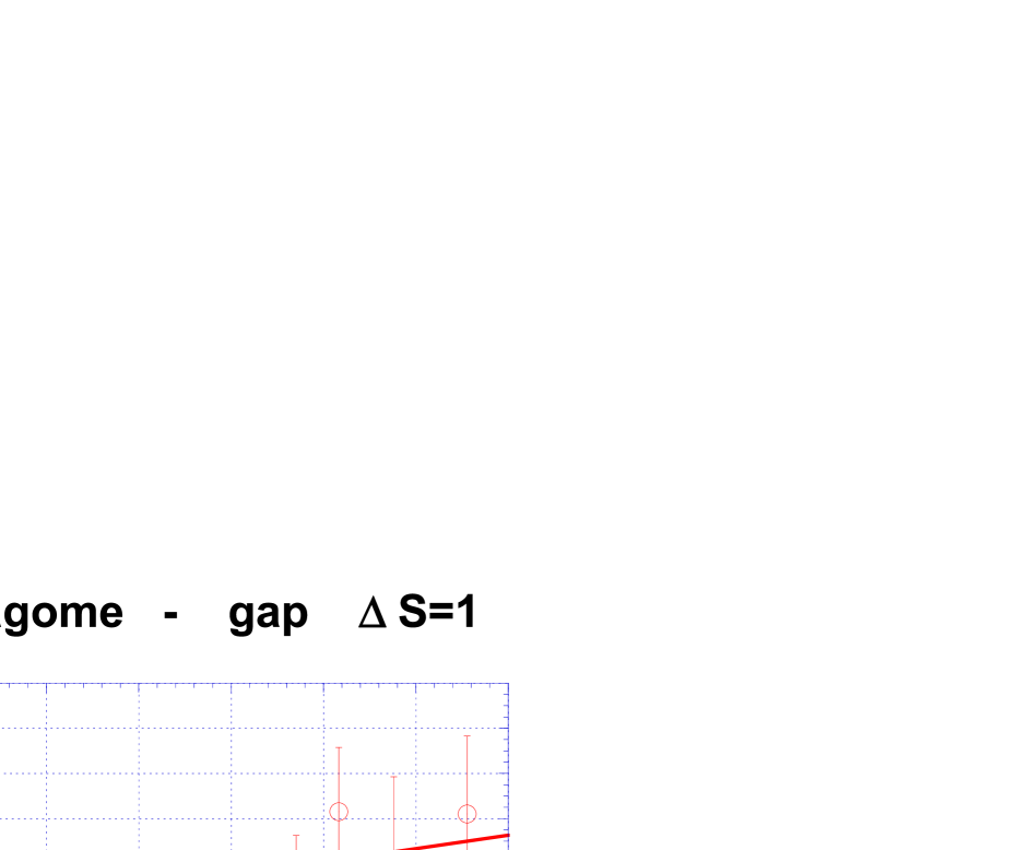
Figure 6.3: Finite size scaling of the spin gap in the spin-1/2 Heisenberg model ${\cal H}=\sum_{<i,j>}{\bf S}_{i}.{\bf S}_{j}$ on the kagome lattice. Data are obtained by the indirect procedure described in the text.

6.2.4 An exceptional density of low lying excitations in the singlet sector

Whatever the ultimate fate of the spin gap a still larger surprise emerges from the exact spectra: the absence of gap in the singlet sector and the anomalous density of low energy states adjacent to the ground-state. We have measured the number of singlet levels in the spin-gap (taken as a natural energy band-width of the problem): this number increases exponentially fast with $N$ as $1.15^{N}$ (see Fig. 6.4).

Figure 6.4: Logarithm of the number of singlet states in the spin gap versus sample size (black squares). The short dashed and long dashed curves display the theoretical law (Eq. 6.5) (short dashes: $p=1$, long dashes: $p=2$).

The first immediate consequence of this property is the existence of a $T=0$ residual entropy in this model. This came as a shock for many scientists who had the idea that the quantum dynamics “should” lift the degeneracy of the incipient Ising model or dimer models (see next section). This does not seem to be the case!!

Some remarks are necessary to fully appreciate this property.

The total number of states of a sample of $N$ spins 1/2 is $2^{N}$. These states are stretched on an energy scale of the order of $NJ$ where $J$ is the coupling constant of the Hamiltonian. This implies that on most of the spectrum the density of states increases exponentially with $N$. If we specialize to the $S=0$ sector as we will do below, the picture is not very different: the number of states is $C^{N}_{\frac{N}{2}}-C^{N}_{\frac{N}{2}-1}\sim{\cal O}(\frac{2^{N}}{N})$ and here too, in most of the spectrum the density is exponentially increasing with N.

BUT in all the phases that we have studied up to now, the nature of the ground-state and of the low lying excitations leads to a different behavior at the edges of the band. Typically the ground-state degeneracy is ${\cal O}(1)$ in VBC and in type I RVBSL and it is ${\cal O}(N^{\alpha})$ in Néel ordered states with $\alpha$ sublattices. In all these situations the low lying excitations can be described as modes or quasi-particles. In the corresponding energy range one typically counts $N^{\beta}$ levels associated with one quasi particle excitations. This always leads to density of states increasing as a power law as a function of $N$. Inclusion of multi-particle excitations can be done in an average way: let us suppose that single particle excitations have a dispersion law:

$$\omega({\bf k})=k^{p}.$$ (6.4)

In a d-dimensional space the internal energy of such a system increases with temperature as $T^{(p+d)/p}$, the specific heat as $T^{d/p}$ as the entropy ${\cal S}$. For a system with $N$ spins the average energy range $W$ excited at the temperature $T$ is of the form: $W=C^{st}NT^{(p+d)/p}$. This implies that the entropy depends on $N$ as: ${\cal S}\propto N\left({\frac{W}{N}}\right)^{\frac{d}{p+d}}$ and thus the average number of excited levels ${\cal N}$ increases as:

$$ln({\cal N})\propto N^{\frac{p}{p+d}}$$ (6.5)

.

As an example, let us consider the quantum critical phase of the Rokhsar Kivelson model on the square lattice at the quantum critical point (Chapter 4 page 60): in that case the critical correlations decrease as $r^{-2}$, the dispersion law is linear in $k$, the logarithm of the number of states increases as $N^{1/3}$ (short dashes of Fig. 6.4), much slower than the exact results.

Even in including many particle excitations one would thus expect a number of levels increasing much more slowly than in the exact results! Except if we accept that there is infinitely soft low energy modes ($p\rightarrow\infty$), then we recover the correct density of low lying levels and a residual entropy. It is still unclear if we can do a connection between the “zero mode” of the classical model at T=0 and this picture. And we cannot completely indulge ourselves in saying that quantum fluctuations are unable to lift the classical degeneracy as quantum fluctuations seems to open a spin gap!

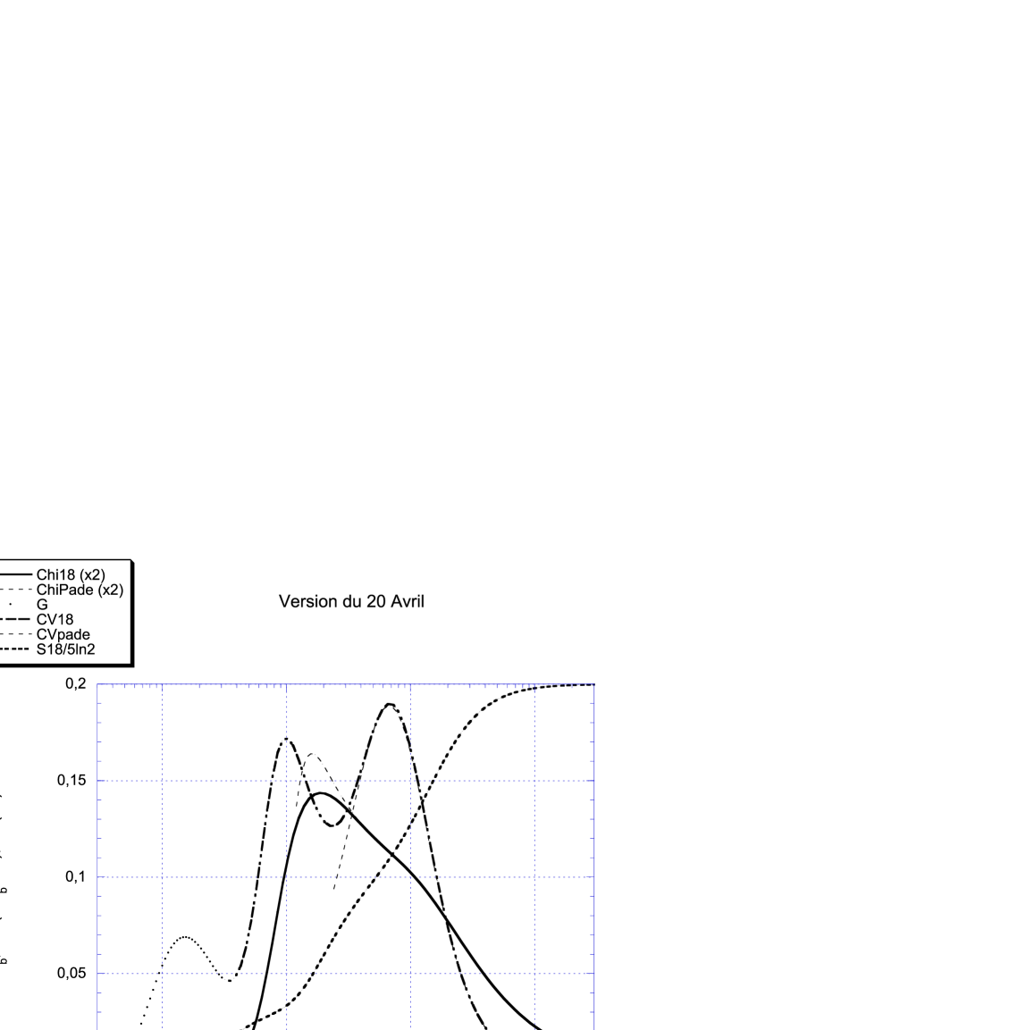
Figure 6.5: Specific heat (dot-dashed curve), entropy (dotted curve) and spin-susceptibility (full line) of the Heisenberg model on the kagome lattice (exact diagonalization on a N=18 sample, and Paddé approximants to high temperature series [147]). The third bump in the specific heat at very low temperature is an artifact of the small size and the associated discretization in the singlet sector. We think that the intermediate bump is a real feature of the specific heat which subsists up to the thermodynamic limit [143]. Note the entropy of the singlets in a range of temperature below the spin gap where the spin excitations are negligible as the spin-susceptibility.

A physical consequence of this exceptional density of low lying singlets can be observed in the specific heat (Fig. 6.5): at low temperature the specific heat of this spin system is unusually insensitive to large magnetic fields. This is easily understood if we suppose that in this energy range the excitations are essentially singlets [143]. This result is to be compared to the experimental results of Ramirez et al. [148] on $SrCrGaO$ where the specific heat around $5K$ has an extremely low sensitivity to magnetic fields up to $10\;Tesla$, whereas the homogeneous susceptibility in this range of temperature is probably very low if we notice that it turns down around $50K$ [149].

6.2.5 Anomalous density of states in other spin sectors

This anomalous density of low lying states has equally been observed in the spin 1/2 sector (where the law could be fitted to $N1.15^{N}$), in the spin 1 sector as well as in other sectors with larger total spin. It should be noticed that such a density of states implies the absence of an intrinsic energy scale for the low lying excitations: a phenomenon that has been observed in inelastic neutron scattering (ref. [150] and refs. therein) and theoretically in the imaginary part of the dynamic susceptibility calculated within the dynamical mean field theory [151]. A very high spin susceptibility just above the spin gap is not excluded in spin-1/2 compounds [152].

6.2.6 Unconfined Spinons

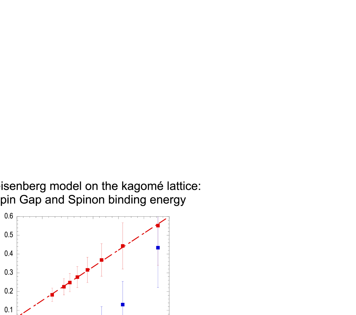
Figure 6.6: Finite size scaling on the spin gap: red squares (raw data) and the spinon binding energy: blue squares (unpublished results).

The spinon binding energy (Fig. 6.6) has been computed in the HK model along the same line as it has been done in Chapter 5 page 75 for the MSE model. The only difference lays in smaller and smoother shape effects in the HK case, which allows to do analytic fit of the energy per spin $e(S_{min},N)$ versus $1/N^{3/2}$ for even and odd samples separately. Eq. 5.6, is then written, with reference to the interpolated value of the energy of even samples for odd value of N: this takes into account the finite size effects with more subtlety than the $(2N+1)e_{\infty}$ term of equation 5.6. All these features explain the smoother behavior of the spinon binding energy shown in Fig. 6.6. From this data one can rather safely conclude that spinons are probably unconfined in the HK model.

The global picture of this phase is thus that of a Spin Liquid, with no long range correlations in local observable, unconfined spinons and a residual entropy of singlets at $T=0$, which is one of the manifestations of an extraordinary large density of states in each $S$ subspace.

6.3 Next-neighbor Resonating Valence Bond description of the spin-1/2 kagome antiferromagnet

Considering a supposed-to-be large spin-gap, Zeng and Elser [140] proposed a description of the ground-state and low lying excitations of the kagome model in the basis of next neighbor Valence Bonds. We know now that the spin gap is certainly smaller than it was expected in 1995, nevertheless Mila and Mambrini [142, 144] have convincingly shown that the picture of a next neighbor resonating Valence Bond Spin liquid captures some of the most perplexing features of this magnet and specifically the absence of gap in the singlet sector and the exponential number of singlets in any given range of energy. This probably implies the absence of an intrinsic low energy scale, which is consistent with the thermal behavior of the dynamic spin susceptibility calculated by Georges and coll. [151]. This feature is typical of a critical state, but as seen in the above discussion, the simple RK picture does not seem to fit nicely to the exact diagonalization data: may be the available sizes are too small or the behavior of this quantum system corresponds to something definitely new.

More generally this picture of the ground-state and first excitations as resonances between an exponential number of dimer coverings gives a qualitatively interesting picture of the low temperature physics of different oxides that can be described as kagome antiferromagnets. The low temperature specific heat of SrCr₉Ga₁₂0₁₉ is apparently dominated by local singlet states [148]. The magnetic excitations of this same compound as seen by muons can be described as spins 1/2 itinerant in a sea of singlets [25]. SrCr₉Ga₁₂0₁₉ exhibits at about 5 K a very large increase of its non linear susceptibility reminiscent of spin glasses [153], but neutrons and muons show that most of the spins are not frozen below this temperature and exhibit still very rapid fluctuations[154]. The same phenomena have been observed in two jarosites that are equally good models of kagome antiferromagnets with half-odd-integer spin per unit cell [155, 156].

6.4 Haldane’s conjecture

Whereas the classical Heisenberg model on the kagome, checker-board and pyrochlore lattices share the property of an extensive entropy and disorder at $T=0$, their quantum counterparts are quite different. As it has been explained in Chapter 4, the Heisenberg model on the checker-board lattice has an ordered Valence Bond Crystal with gaps to all excitations.

Less is known on the ground-state of the Heisenberg model on the 3-dimensional pyrochlore lattice: Canals and Lacroix [157] have shown that their spin-spin correlations are short ranged and they have seen on a 16 sites spectrum that the first excitations were singlet ones. Having done the spectrum of a 32 sites pyrochlore sample, we confirm that the first excitations are still singlets for this size. But the finite size effects on these excitations between 16 and 32 are very large and it remains possible that the gap in the singlet sector be larger than the singlet-triplet gap in the thermodynamic limit [fmsl03, f03]: in any case there is definitely a gap in the singlet sector in this last model!

On the other hand, recent results from Hida [160] show that there is a gap to all excitations in the S=1 HK model.

All these results seem to confirm Haldane’s conjecture: among these strongly frustrated systems with an extensive degeneracy in the classical limit the spin-1/2 kagome antiferromagnet is the only system to have an half-odd-integer spin in the unit cell and gapless excitations. The spin-1/2 Heisenberg model on the checkerboard lattice or on the pyrochlore lattice and the spin-1 Heisenberg model on the kagome lattice have integer spins in the unit cell and quantum fluctuations lead to gapful excitations.

Acknowledgements Ce texte représente des notes accompagnant un cours donné à l’automne 2002 à Lausanne dans le cadre des cours de troisième cycle de l’École de Physique Romande sur invitation du Pr. F. Mila. Une partie notable des résultats provient du travail de recherche fait à Paris par mes collègues, étudiants en thèse et post-doc: B. Bernu, J.-C. Domenge, J. B. Fouet, P. Lecheminant, G. Misguich, L. Pierre, et d’une fructueuse collaboration avec C. Waldtmann et le Pr. H.-U. Everts. Que tous soient remerciés. Un article de revue rédigé par G. Misguich et C. L. donnant un point de vue moins auto-centré et plus récent est disponible sur le serveur d’archives: cond-mat/0310405

Bibliography

- [1] D. C. Mattis, The Theory of Magnetism I, Vol. 17 of Springer Series in Solid-State Sciences (Springer-Verlag, Berlin, Heidelberg, New York, Tokyo, 1981).
- [2] W. J. Caspers, Spin Systems (World Scientific, Singapore, 1989).
- [3] A. Auerbach, Interacting electrons and Quantum Magnetism (Springer-Verlag, Berlin Heidelberg New York, 1994).
- [4] Hulthen, Ark. Mat. Astron. Fys. 26A, 1 (1938).
- [5] W. Marshall, Proc. Roy. soc. London A 232, 48 (1955).
- [6] E. H. Lieb and D. Mattis, J. of Math. Phys. 3, 749 (1962).
- [7] P. Anderson, Phys. Rev. 86, 694 (1952).
- [8] P. Anderson, Concept in Solids (Benjamin, New York, 1963).
- [9] P. Anderson, Basic Notions of Condensed Matter Physics (Benjamin, New York, 1984).
- [10] B. Bernu, C. Lhuillier, and L. Pierre, Phys. Rev. Lett. 69, 2590 (1992).
- [11] B. Bernu, P. Lecheminant, C. Lhuillier, and L. Pierre, Phys. Rev. B 50, 10048 (1994).
- [12] P. Lecheminant, Ph.D. thesis, Université Pierre et Marie Curie, Paris, 95.
- [13] R. Kubo, Phys. Rev 87, 568 (1952).
- [14] T. Kennedy, E. Lieb, and B. Shastry, J. Stat. Phys. 53, 1019 (1988).
- [15] F. Dyson, E. Lieb, and B. Simon, J. Stat. Phys. 18, 335 (1978).
- [16] E. J. Neves and J. F. Perez, Phys. Lett. 114A, 331 (1986).
- [17] I. Affleck, T. Kennedy, E. H. Lieb, and H. Tasaki, Commun. Math. Phys. 115, 477 (1988).
- [18] P. Anderson, Mater. Res. Bull. 8, 153,160 (1973).
- [19] P. Fazekas and P. Anderson, Philos. Mag. 30, 423 (1974).
- [20] J.-B. Fouet, P. Sindzingre, and C. Lhuillier, Eur. Phys. J. B 20, 241 (2001).
- [21] P. Tomczak and J. Richter, Phys. Rev. B 59, 107 (1999).
- [22] N. Trivedi and D. Ceperley, Phys. Rev. B 41, 4552 (1990).
- [23] C. Waldtmann et al., Eur. Phys. J. B 2, 501 (1998).
- [24] J.-B. Fouet, M. Mambrini, P. Sindzingre, and C. Lhuillier, cond-mat/0108070 (unpublished).
- [25] Y. Uemura et al., Phys. Rev. Lett. 73, 3306 (1994).
- [26] M. Gross, E. Sanchez-Velasco, and E. Siggia, Phys. Rev. B 39, 2484 (1989).
- [27] M. Gross, E. Sanchez-Velasco, and E. Siggia, Phys. Rev. B 40, 11328 (1989).
- [28] H. Neuberger and T. Ziman, Phys. Rev. B 39, 2608 (1989).
- [29] D. Fisher, Phys. Rev. B 39, 11783 (1989).
- [30] P. Azaria, B. Delamotte, and D. Mouhanna, Phys. Rev. Lett. 70, 2483 (1993).
- [31] P. Hasenfratz and F. Niedermayer, Z. Phys. B. Condensed Matter 92, 91 (1993).
- [32] J. C. Domenge, rapport de DEA, Magistere des Sciences de la matière de Lyon, 2002 (unpublished).
- [33] A. Sütö and P. Fazekas, Phil. Mag. 35, 623 (1977).
- [34] G. Levine and J. Howard, Phys. Rev. Lett. 75, 4142 (1995).
- [35] P. Lecheminant, B. Bernu, C. Lhuillier, and L. Pierre, Phys. Rev. B 52, 6647 (1995).
- [36] J.-B. Fouet, Ph.D. thesis, Université Cergy Pontoise, 2002.
- [37] J. Villain, R. Bidaux, J. Carton, and R. Conte, J. Phys. Fr. 41, 1263 (1980).
- [38] E. Shender, Sov. Phys. J.E.T.P. 56, 178 (1982).
- [39] T. Oguchi, H. Nishimori, and Y. Taguchi, J. Phys. Soc. Jpn. 54, 4494 (1985).
- [40] C. L. Henley, Phys. Rev. Lett. 62, 2056 (1989).
- [41] E. Dagotto and A. Moreo, Phys. Rev. Lett. 63, 2148 (1989).
- [42] T. Jolicoeur, E. Dagotto, E. Gagliano, and S. Bacci, Phys. Rev. B 42, 4800 (1990).
- [43] A. Chubukov and T. Jolicoeur, Phys. Rev. B 46, 11137 (1992).
- [44] S. E. Korshunov, Phys. Rev. B 47, 6165 (1993).
- [45] R. Deutscher and H. Everts, Z. Phys. B. Condensed Matter 93, 77 (1993).
- [46] H. Schultz and T. Ziman, Europhys. Lett. 8, 355 (1992).
- [47] M. E. Zhitomirsky and K. Ueda, Phys. Rev. B 54, 9007 (1996).
- [48] V. N. Kotov, J. Oitmaa, O. Sushkov, and Z. Weihong, cond-mat/9912228 (unpublished).
- [49] V. N. Kotov, J. Oitmaa, O. Sushkov, and Z. Weihong, Phys. Rev. B 60, 14613 (1999).
- [50] L. Capriotti and S. Sorella, Phys. Rev. Lett. 84, 3173 (2000).
- [51] L. Capriotti, F. Becca, A. Parola, and S. Sorella, Phys. Rev. Lett. 87, 097201 (2001).
- [52] S. Palmer and J. Chalker, Phys. Rev. B 64, 094412 (2002).
- [53] W. Brenig and A. Honecker, Phys. Rev. B 65, 140407R (2002), cond-mat/0111405.
- [54] E. Berg, E. Altman, and A. Auerbach, cond-mat/0206384 (unpublished).
- [55] B. Shastry and B. Sutherland, Physica B (Amsterdam) 108, 1069 (1981).
- [56] T. Momoi and K. Totsuka, Phys. Rev. B 62, 15067 (2000).
- [57] N. Katoh and M. Imada, J. Phys. Soc. Jpn. 63, 4529 (1994).
- [58] M. Troyer, H. Tsnunetsgu, and D. Wurte, Phys. Rev. B 50, 13515 (1994).
- [59] S. Taniguchi et al., J. Phys. Soc. Jpn. 64, 2758 (1995).
- [60] Y. Fukumoto and A. Oguchi, J. Phys. Soc. Jpn. 65, 1440 (1996).
- [61] M. Albrecht and F. Mila, Europhys. Lett 34, 145 (1996).
- [62] M. Albrecht and F. Mila, Phys. Rev. B 53, 2945 (1996).
- [63] T. Miyasaki and D. Yoshioka, J. Phys. Soc. Jpn. 65, 2370 (1996).
- [64] S. Sachdev and N. Read, Phys. Rev. Lett. 77, 4800 (1996).
- [65] K. Ueda, H. Kontani, M. Sigrist, and P. A. Lee, Phys. Rev. Lett. 76, 1932 (1996).
- [66] K. Kodama et al., J. Phys. Soc. Jpn. 65, 1941 (1996).
- [67] M. Troyer, H. Kontani, and K. Ueda, Phys. Rev. Lett. 76, 3822 (1996).
- [68] K. Kodama et al., J. Phys. Soc. Jpn. 66, 28 (1997).
- [69] T. Ohama, H. Yasuoka, M. Isobe, and Y. Ueda, J. Phys. Soc. Jpn. 66, 23 (1997).
- [70] H. Kageyama et al., Phys. Rev. Lett. 82, 3168 (1999).
- [71] S. Miyahara and K. Ueda, Phys. Rev. Lett. 82, 3701 (1999).
- [72] Z. Weihong, C. J. Hamer, and J. Oitmaa, Phys. Rev. B 60, 6608 (19999).
- [73] O. Cepas et al., J. Phys. Soc. Jpn. 68, 2906 (1999).
- [74] S. Miyahara and K. Ueda, Phys. Rev. B 61, 3417 (2000).
- [75] A. Koga and N. Kawakami, Phys. Rev. Lett. 84, 4461 (2000).
- [76] C. H. Chung, J. B. Marston, and S. Sachdev, cond-mat/0102222 (unpublished).
- [77] E. Müller-Hartmann, R. R. P. Singh, C. Knetter, and G. S. Uhrig, Phys. Rev. Lett. 84, 1808 (2000).
- [78] O. Cepas et al., Phys. Rev. Lett. 87, 167205 (2001).
- [79] D. Rokhsar and S. Kivelson, Phys. Rev. Lett. 61, 2376 (1988).
- [80] J. Chayes, L. Chayes, and S. Kivelson, Commun. Math. Physic. 123, 53 (1989).
- [81] G. Misguich, C. Lhuillier, M. Mambrini, and P. Sindzingre, Eur. Phys. J. B 26, 167 (2002), cond-mat/0112360.
- [82] M. Kohmoto and Y. Shapir, Phys. Rev. B 37, 9439 (1988).
- [83] M. E. Fisher and J. Stephenson, Phys. Rev. 132, 1411 (1963).
- [84] S. Sachdev, Phys. Rev. B 40, 5204 (1989).
- [85] P. Leung, K. Chiu, and K. Runge, Phys. Rev. B 54, 12938 (1996).
- [86] E. Fradkin, in Field Theories of Condensed Matter Systems, Frontiers in Physics, edited by D. Pines (Addison-Wesley, USA, 1991).
- [87] R. Moessner and S. L. Sondhi, Phys. Rev. Lett. 86, 1881 (2001).
- [88] I. Affleck and J. Marston, Phys. Rev. B 37, 3774 (1988).
- [89] N. Read and S. Sachdev, Phys. Rev. Lett. 62, 1694 (1989).
- [90] S. Liang, B. Doucot, and P. Anderson, Phys. Rev. Lett. 61, 365 (1988).
- [91] B. Sutherland, Phys. Rev. B 37, 3786 (1988).
- [92] B. Sutherland, Phys. Rev. B 38, 7192 (1988).
- [93] N. Read and B. Chakraborty, Phys. Rev. B 40, 7133 (1989).
- [94] R. Coldea, D. A. Tennant, A. M. Tsvelick, and Z. Tylczynski, Phys. Rev. Lett. 86, 1335 (2001).
- [95] S. Sachdev, Phys. Rev. B 45, 12377 (1992).
- [96] G. Misguich, B. Bernu, C. Lhuillier, and C. Waldtmann, Phys. Rev. Lett. 81, 1098 (1998).
- [97] G. Misguich, C. Lhuillier, B. Bernu, and C. Waldtmann, Phys. Rev. B 60, 1064 (1999).
- [98] D. Thouless, Proc. Phys. Soc. 86, 893 (1965).
- [99] M. Roger, J. Hetherington, and J. Delrieu, Rev. Mod. Phys. 55, 1 (1983).
- [100] C. Herring, in Magnetism, edited by G. T. Rado and H. Suhl (Academic Press, New York and London, 1966), p. vol IV.
- [101] M. Roger et al., Phys. Rev. Lett. 80, 1308 (1998).
- [102] E. Collin et al., Phys. Rev. Lett. 86, 2447 (2001).
- [103] B. Bernu, L. Candido, and D. Ceperley, Phys. Rev. Lett. 86, 870 (2001).
- [104] R. Coldea et al., Phys. Rev. Lett. 86, 5377 (2001).
- [105] A. Katanin and A. Kampf, cond-mat/0111533 (unpublished).
- [106] A. Läuchli, G. Schmid, and M. Troyer, cond-mat/0206153, and oral communication March Meeting 2002, Indianapolis (unpublished).
- [107] W. LiMing, G. Misguich, P. Sindzingre, and C. Lhuillier, Phys. Rev. B 62, 6372,6376 (2000).
- [108] G. Misguich, Ph.D. thesis, Université Pierre et Marie Curie. Paris. France, 1999.
- [109] M. Oshikawa, Phys. Rev. Lett. 84, 1535 (2000).
- [110] A. Y. Kitaev, quant-phys/9707021 (unpublished).
- [111] L. B. Ioffe et al., Nature 415, 503 (2002), cond-mat/0111224.
- [112] S. Kivelson, cond-mat/0106126 (unpublished).
- [113] C. Nayak and K. Shtengel, Phys. Rev. B 64, 064422 (2001).
- [114] K. Park and S.Sachdev, Phys. Rev. B 65, 220405 (2002), cond-mat/0112003.
- [115] T. Senthil, cond-mat/0105104 and refs. therein (unpublished).
- [116] L. Balents, M. P. A. Fisher, and S. M. Girvin, Phys. Rev. B 65, 224412 (2002).
- [117] E. Demler et al., Phys. Rev. B 65, 155103 (2002).
- [118] R. Moessner, S. L. Sondhi, and E. Fradkin, Phys. Rev. B 65, 024504 (2002).
- [119] N. E. Bonesteel, Phys. Rev. B 40, 8954 (1989).
- [120] X. Wen, Phys. Rev. B 44, 2664 (1991).
- [121] S. Sachdev and K. Park, Annals of Physics (N.Y.) 58, 298 (2002), cond-mat/0108214.
- [122] F. Haldane, Phys. Rev. Lett. 55, 2095 (1985).
- [123] X. Wen and Q. Niu, Phys. Rev. B 41, 9377 (1990).
- [124] G. Santoro et al., Phys. Rev. Lett. 83, 3065 (1999), we acknowledge a very interesting exchange on this subject in Trieste.
- [125] R. Moessner and S. L. Sondhi, Phys. Rev. B 63, 224401 (2001).
- [126] J. Kogut, Rev. Mod. Phys. 51, 659 (1979).
- [127] C. Lannert, M. P. A. Fisher, and T. Senthil, Phys. Rev. B 63, 134510 (2001).
- [128] T. Senthil and M. P. A. Fisher, Phys. Rev. B 63, 134521 (2001).
- [129] L. Pauling, in The nature of the chemical bond (Cornell University Press, Ithaca, 1938).
- [130] K. Kano and S. Naya, Progress in Theoretical physics 10, 158 (1953).
- [131] D. Huse and A. Rutenberg, Phys. Rev. B 45, 7536 (1992).
- [132] R. Moessner, S. L. Sondhi, and P. Chandra, Phys. Rev. Lett. 84, 4457 (2000).
- [133] J. Chalker, P. C. W. Holdsworth, and E. F. Shender, Phys. Rev. Lett. 68, 855 (1992).
- [134] I. Richtey, P. Chandra, and P. Coleman, Phys. Rev. B 47, 15342 (1993).
- [135] M. Elhajal, Ph.D. thesis, Université Joseph Fourier. Grenoble. France, 2002.
- [136] M. Elhajal, B. Canals, and C. Lacroix, cond-mat/0202194 (unpublished).
- [137] V. Elser, Phys. Rev. Lett. 62, 2405 (1989).
- [138] J. Chalker and J. Eastmond, Phys. Rev. B 46, 14201 (1992).
- [139] P. Leung and V. Elser, Phys. Rev. B 47, 5459 (1993).
- [140] C. Zeng and V. Elser, Phys. Rev. B 51, 8318 (1995).
- [141] P. Lecheminant et al., Phys. Rev. B 56, 2521 (1997).
- [142] F. Mila, Phys. Rev. Lett. 81, 2356 (1998).
- [143] P. Sindzingre et al., Phys. Rev. Lett. 84, 2953 (2000).
- [144] M. Mambrini and F. Mila, Eur. Phys. J. B 17, 651,659 (2001).
- [145] C. Lhuillier and G. Misguich, in High Magnetic Fields, edited by C. Berthier, L. Levy, and G. Martinez (Springer, Berlin, 2002), pp. 161–190, cond-mat/0109146.
- [146] K. Hida, J. of the Phys. Soc. of Japan 70, 3673 (2001).
- [147] N. Eltsner and A. P. Young, Phys. Rev. B 50, 6871 (1994).
- [148] A. P. Ramirez, B. Hessen, and M. Winkelmann, Phys. Rev. Lett. 84, 2957 (2000).
- [149] P. Mendels et al., Phys. Rev. Lett. 85, 3496 (2000).
- [150] T. Mondelli et al., Physica B 284, 1371 (2000).
- [151] A. Georges, R. Siddhartan, and S. Florens, Phys. Rev. Lett. 87, 277203 (2001).
- [152] C. Lhuillier and P. Sindzingre, in Quantum properties of Low dimensional antiferromagnets, edited by Y. Ajiro and J. P. Boucher (Kyushu University Press, Fukuoka, Japan, 2002), p. 111, iSBN 4 87378 740 8.
- [153] A. Ramirez, G. P. Espinosa, and A. S. Cooper, Phys. Rev. Lett. 64, 2070 (1990).
- [154] S.-H. Lee et al., Europhys. Lett 35, 127 (1996).
- [155] A. Keren et al., Phys. Rev. B 53, 6451 (1996).
- [156] A. S. Wills et al., Europhys. Lett 42, 325 (1998).
- [157] B. Canals and C. Lacroix, Phys. Rev. Lett. 80, 2933 (1998).
- [158] H. Tsunetsgu, J. Phys. Soc. Jpn. 70, 640 (2001).
- [159] H. Tsunetsgu, Phys. Rev. B 65, 024415 (2002).
- [160] K. Hida, J. of the Phys. Soc. of Japan 69, 4003 (2000).