Survival of a Diffusing Particle in a Transverse Flow Field

Abstract

We consider a particle diffusing in the $y$-direction, $dy/dt=\eta(t)$ where $\eta(t)$ is Gaussian white noise, and subject to a transverse flow field in the $x$-direction, $dx/dt=f(y)$, where $x\geq 0$ and $x=0$ is an absorbing boundary. We discuss the time-dependence of the survival probability of the particle for a class of functions $f(y)$ that are positive in some regions of space and negative in others.

PACS numbers: 02.50.-r, 05.40.-a

I Introduction

In a recent paper [1] we considered a class of stochastic processes defined by the equations

$$\dot{y} = \eta(t)\ ,$$ (1)

$$\dot{x} = f(y),$$ (2)

where $\eta(t)$ is Gaussian white noise with mean zero and correlator $\langle\eta(t)\eta(t^{\prime})\rangle=2D\delta(t-t^{\prime})$. Equations (1) and (2) represent a particle which diffuses (performs a random walk) in the $y$-direction but is subject to a deterministic drift in the $x$-direction with a $y$-dependent drift velocity. We consider the case where there is an absorbing boundary at $x=0$, and we are interested in the survival probability of the particle. Two previously studied models are the cases $f(y)=y$ and $f(y)={\rm sgn}(y)$. The former is equivalent to the random acceleration process, $\ddot{x}=\eta(t)$, while the latter is the ‘windy cliff’ model introduced by Redner and Krapivsky [2]. For both these models, the survival probability of the particle decays as $t^{-1/4}$ for large time $t$, and it has been argued [1, 2] that this is a generic result for odd functions $f(y)$. It should be noted that, in general, such problems are highly nontrivial and exact solutions are available in only a small number of cases.

In ref.[1], we raised the question of how the survival probability decays when the function $f(y)$ is not an odd function. We considered a class of models where $f(y)=v_{+}y^{\alpha}$ for $y>0$, and $f(y)=-v_{-}(-y)^{\alpha}$ for $y<0$. Here the drift takes the particle away from the absorbing boundary for $y>0$, and towards it for $y<0$, but not in a symmetrical way: the function $f(y)$ is odd only when $v_{+}=v_{-}$. Using an extension of a technique developed by Burkhardt [3] in connection with the random acceleration process, we showed that the survival probability decays as $t^{-\theta}$ for large $t$, where the exponent $\theta$ (the ‘persistence exponent’) is nontrivial and given by

$$\theta=\frac{1}{4}-\frac{1}{2\pi\beta}\tan^{-1}\left[\frac{v_{+}^{\beta}-v_{-}^{\beta}}{v_{+}^{\beta}+v_{-}^{\beta}}\tan\left(\frac{\pi\beta}{2}\right)\right]$$ (3)

where $\beta=1/(2+\alpha)$. This reduces to $\theta=1/4$ for $v_{+}=v_{-}$ but $\theta$ lies in the range $0<\theta<1/2$ in general. When $v_{+}>v_{-}$, the drift away from the boundary is weakly dominant. The decay of the survival probability still has a power law form, but $\theta<1/4$, while the converse occurs for $v_{+}<v_{-}$: the drift toward the boundary is weakly dominant and $\theta>1/4$. The fact that $1/2$ is an upper bound for $\theta$ is clear when one recalls that the probability that the particle stays in the region $y>0$ (and therefore never encounters the drift towards the absorbing boundary) decays as $t^{-1/2}$ [4, 5].

It is worth emphasising that the process defined by Eqs. (1) and (2) is non-Gaussian except when $f(y)$ is linear. Eq. (3) is a rare example of an exactly calculable persistence exponent for a non-Gaussian process.

In [1] we speculated about the behavior of the system when the function $f(y)$ is described by different exponents, $\alpha_{+}$ and $\alpha_{-}$, for $y>0$ and $y<0$ respectively. We argued that for $\alpha_{+}>\alpha_{-}$ the drift away from the boundary is strongly dominant, leading to a non-zero survival probability at infinite time (i.e. $\theta=0$) , while for $\alpha_{+}<\alpha_{-}$ the drift towards the boundary is strongly dominant and $\theta$ obtains its maximum value of $1/2$.

In the present work we obtain some exact result pertinent to the latter question. Looking at the case $\alpha_{+}>\alpha_{-}$, we show explicitly that the survival probability approaches a non-zero value at infinite time and we obtain a closed-form expression for this value.

In the second part of the paper we revisit the issue of whether the decay exponent $\theta$ takes the value $1/4$ for all odd functions $f(y)$, as has been assumed up to now. We consider models where the flow field takes a periodic, banded form with $f(y)$ taking the values $v_{+}$ and $-v_{-}$ in alternate bands of width $b_{+}$, $b_{-}$ respectively. We demonstrate numerically that for the case $b_{+}=b_{-}$ and $v_{+}=v_{-}$ which, with appropriate cloice of the $y=0$ axis, represents an odd function, $\theta=1/2$, not $1/4$ and we argue that $\theta=1/2$ whenever there is no net drift, i.e. when $v_{+}b_{+}=v_{-}b_{-}$. In these cases we argue that an effective diffusion in the $x$-direction, resulting from the stochastic movement between the alternating bands, dominates over the drift and naturally accounts for the exponent $1/2$. We obtain an analytical result in the limit $b_{-}\to 0$, $v_{-}\to\infty$, with $b_{-}v_{-}$ held fixed and equal to $b_{+}v_{+}$, and we verify that $\theta=1/2$ in this case.

II Model and Calculation

The model we consider initially is defined by Eqs. (1) and (2), with the function $f(y)$ given by

$$f(y)=\cases{v_{+}y^{\alpha_{+}},\ \ \ \ \ \ \ \ \ \ y>0,\cr-v_{-}(-y)^{\alpha_{-}},\ \ \ y<0.\cr}$$ (4)

We work in the regime $\alpha_{+}>\alpha_{-}$, where we expect a non-zero survival probability. The probability, $Q(x,y)$ that the particle survives to infinite time satisfies the backward Fokker-Planck equation (BFPE) $D\partial_{yy}Q+f(y)\partial_{x}Q=0$. In the present context it is convenient to work instead with the ‘killing probability’, $P=1-Q$, which obviously satisfies the same equation,

$$D\partial_{yy}P+f(y)\,\partial_{x}P=0\ ,$$ (5)

but with different boundary conditions. The boundary conditions on $P(x,y)$ are

$$P(\infty,y) = 0,$$ (6)

$$P(x,\infty) = 0,$$ (7)

$$P(0,y) = 1,\ \ y<0\ ,$$ (8)

the last of these following from the fact that, for an initial condition with $x=0$ and $y<0$, the flow immediately takes the particle on to the absorbing boundary.

Inserting the form (4) for $f(y)$ in (5), the equation can be solved separately in each regime by separation of variables. Imposing the boundary conditions (6) and (7) the result takes the form (setting $D=1$ for convenience)

$$P(x,y) = \sqrt{y}\int_{0}^{\infty}dk\,a(k)K_{\beta_{+}}\left(2\beta_{+}\sqrt{kv_{+}}y^{1/2\beta_{+}}\right)\,e^{-kx},$$ (10)

$$\hskip 128.0374pt{\rm for}\ y>0,$$

$$= \sqrt{-y}\int_{0}^{\infty}dk\,\left\{b(k)J_{\beta_{-}}\left(2\beta_{-}\sqrt{kv_{-}}(-y)^{1/2\beta_{-}}\right)\right.$$ (13)

$$\hskip 5.69046pt+\left.c(k)J_{-\beta_{-}}\left(2\beta_{-}\sqrt{kv_{-}}(-y)^{1/2\beta_{-}}\right)\right\}\,e^{-kx},$$

$$\hskip 128.0374pt{\rm for}\ y<0,$$

where

$$\beta_{\pm}=1/(2+\alpha_{\pm}),$$ (14)

$J_{\nu}(z)$ is a Bessel function and $K_{\nu}(z)$ a modified Bessel function.

Eqs.  (10) and (13) contain the three undetermined functions $a(k)$, $b(k)$ and $c(k)$. The last two can be expressed in terms of $a(k)$ by imposing suitable continuity conditions at $y=0$. From the BFPE, Eq. (5), it follow that both $P(x,y)$ and $\partial_{y}P(x,y)$ are continuous at $y=0$. Imposing these conditions gives the relations

$$b(k) = K_{b}\,k^{(\beta_{+}-\beta_{-})/2}\,a(k),$$ (15)

$$c(k) = K_{c}\,k^{(\beta_{-}-\beta_{+})/2}\,a(k),$$ (16)

where

$$K_{b} = \frac{\pi}{2\sin(\beta_{+}\pi)}\frac{\Gamma(1+\beta_{-})}{\Gamma(1+\beta_{+})}\frac{\left(\beta_{+}\sqrt{v_{+}}\right)^{\beta_{+}}}{\left(\beta_{-}\sqrt{v_{-}}\right)^{\beta_{-}}},$$ (17)

$$K_{c} = \frac{1}{2}\,\Gamma(\beta_{+})\Gamma(1-\beta_{-})\frac{\left(\beta_{-}\sqrt{v_{-}}\right)^{\beta_{-}}}{\left(\beta_{+}\sqrt{v_{+}}\right)^{\beta_{+}}}.$$ (18)

Finally, $a(k)$ is determined by the boundary condition (8). This gives

$$1 = \sqrt{-y}\int_{0}^{\infty}dk\,\left\{b(k)J_{\beta_{-}}\left(2\beta_{-}\sqrt{kv_{-}}(-y)^{1/2\beta_{-}}\right)\right.$$ (20)

$$+\left.c(k)J_{-\beta_{-}}\left(2\beta_{-}\sqrt{kv_{-}}(-y)^{1/2\beta_{-}}\right)\right\},\ \ \ y<0.$$

In principle, Eqs.  (15), (16) and (20) completely determine the functions $a(k)$, $b(k)$ and $c(k)$. In practice, however, we have been unable to extract these functions explicitly. We can, however, determine the small-$k$ forms. These are sufficient to demonstrate our main claims.

To determine the small-$k$ behavior of $a(k)$ we consider Eq. (20) in the limit $y\to-\infty$, since the integral is dominated by small values of $k$ in that limit. We make the ansatz

$$a(k)\sim Ak^{a},\ \ \ k\to 0\ .$$ (21)

Then the small-$k$ forms of $b(k)$ and $c(k)$ are fixed by equations (15) and (16). Since $\beta_{+}<\beta_{-}$, $b(k)\gg c(k)$ for $k\to 0$, so the first term, involving $b(k)$, in Eq. (20) dominates for large negative $y$, and the term involving $c(k)$ is negligible. In this limit, therefore, Eq. (20) reads

$$1 = AK_{b}\lim_{y\to-\infty}\sqrt{-y}\int_{0}^{\infty}dk\,k^{a+(\beta_{+}-\beta_{-})/2}$$ (23)

$$\hskip 56.9055pt\times J_{\beta_{-}}\left(2\beta_{-}\sqrt{kv_{-}}(-y)^{1/2\beta_{-}}\right).$$

Evaluating the integral fixes the values of the exponent $a$ and the amplitude $A$ in Eq. (21):

$$a = \beta_{-}-\frac{\beta_{+}}{2}-1,$$ (24)

$$A = \frac{(\beta_{-}\sqrt{v_{-}})^{\beta_{-}}}{K_{b}\Gamma(\beta_{-})}.$$ (25)

Inserting the small-$k$ results for $a(k)$, $b(k)$ and $c(k)$ in Eqs. (10) and (13) determines $P(x,y)$ in the entire regime where $x$ or $y$ (or both) are large. Especially simple is the limit of large $x$ at $y=0$, where one obtains

$$P(x,0)\sim\frac{\Gamma(\beta_{+})\Gamma(\beta_{-}-\beta_{+})}{2K_{b}\Gamma(\beta_{-})}\,\frac{(\beta_{-}\sqrt{v_{-}})^{\beta_{-}}}{(\beta_{+}\sqrt{v_{+}})^{\beta_{+}}}\,\frac{1}{x^{\beta_{-}-\beta_{+}}},$$ (26)

for $x\to\infty$. This result demonstrates that there is a non-zero infinite-time survival probability provided $\beta_{-}>\beta_{+}$, i.e. $\alpha_{+}>\alpha_{-}$. The spatial decay exponent, $\beta_{-}-\beta_{+}$, should have (we feel) a simple physical derivation, but so far it has eluded us.

III Periodic flow fields

In the remaining part of this paper we consider the case where $f(y)$ is a periodic function of $y$, with period $2b$. In particular, we consider the case

$$f(y)=\cases{v,\ \ \ \ \ \ 2nb<y<(2n+1)b,\cr-v,\ \ \ \ (2n-1)b<y<2nb.\cr}$$ (27)

for all integers $n$. This function $f(y)$ is odd, but we shall show that the survival probability decays asymptotically as $t^{-1/2}$.

We first present, in Figure 1, the result of a numerical simulation for different values of the width, $b$, of the alternating bands. In each case the particle is initially located at $x=0$, on the interface between two bands. To avoid immediate absorption, the first step is taken into the band with positive velocity. For early times, $t\ll b^{2}/D$, the particle explores the two bands either side of the initial position and the decay exponent $1/4$, appropriate to infinitely wide bands is obtained. At time $t\sim b^{2}/D$, however, where the particle starts to explore many bands, there is a clear crossover from the initial $t^{-1/4}$ decay to an asymptotic $t^{-1/2}$ decay.

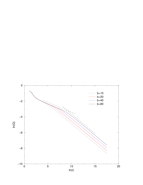
FIG. 1.: Double logarithmic plot of the survival probability $Q$ against time $t$ for a range of band widths $b$. The data show, after a short-time transient, an initial $t^{-1/4}$ decay crossing over to a $t^{-1/2}$ decay at later times. The dashed lines with slopes $-1/4$ and $-1/2$ are guides to the eye.

To understand these results, we first recall the use of the Sparre Anderson theorem [6] to demonstrate that $\theta=1/4$ for odd functions $f(y)$. First suppose that $f(y)>0$ for $y>0$ and $f(y)<0$ for $y<0$. We focus on crossings of the $x$-axis and regard the steps between crossings as the elementary steps of a one-dimensional random walk on the $x$-axis. The steps are clearly (i) independent, and (ii) drawn from a symmetric distribution. The Sparre Anderson theorem states that the probability that the process has not crossed the absorbing boundary at $x=0$ after $N$ steps decays as $Q_{N}\sim N^{-1/2}$ for large $N$. Since the number of crossings in time $t$ scales as $N\sim t^{1/2}$, this implies $Q(t)\sim t^{-1/4}$.

Let us examine this argument more carefully. It’s validity clearly requires that a crossing of the absorbing boundary at $x=0$ can occur at most once between two consecutive crossings of the $x$-axis. This will always be the case if $f(y)$ takes only one sign for $y>0$ and the other sign for $y<0$. In the periodic case, however, $f(y)$ takes both signs for $y>0$ and both signs for $y<0$. The process can therefore cross the absorbing boundary, from $x>0$ to $x<0$, and cross back again without crossing the $x$-axis. Such absorption process will be missed in a description which focuses only on crossings of the $x$-axis. Such a description will typically underestimate the value of $\theta$ (it gives a lower bound on $\theta$).

A better way of looking at this problem is as follows. The probability $Q(x,y,t)$ that the particle survives until time $t$, given that it started at $(x,y)$, is periodic with period $2b$. In particular, the partial derivative $\partial_{y}Q$ vanishes by symmetry at the center of any band. It therefore suffices to solve the problem in the region $-b/2\leq y\leq b/2$, $x\geq 0$, which defines a semi-infinite strip, with boundary conditions $Q(0,y,t)=0$, $\partial_{y}Q(x,\pm b/2,t)=0$. The flow velocity is $v$ in the upper part of the strip ($y>0$) and $-v$ in the lower part. This strip problem has been discussed by Redner and Krapivsky [2], who argue as follows. The typical time between crossings of the center line, $y=0$, is $\tau\sim b^{2}/D$. The typical distance travelled, in the $x$-direction, in this time is $l\sim vb^{2}/D$. The two cases $x\gg l$ and $x\ll l$, where $x$ is the initial displacement of the particle, have to be analysed separately. The following discussion is based on reference [2].

A The regime $x\gg l$

The crossings of the $x$-axis define a symmetric one-dimensional random walk with step length $\sim l$ and time step $\sim\tau$. The effective diffusion constant for motion in the $x$-direction is, therefore, $D_{\parallel}\sim l^{2}/\tau\sim v^{2}b^{2}/D$. The survival probability for this random walk is given by the well-known result [4]

$$Q(x,y,t)\sim\frac{x}{\sqrt{D_{\parallel}t}}\sim\frac{x}{bv}\sqrt{\frac{D}{t}}.$$ (28)

Note that the $y$-dependence is not determined by this argument. It is intuitively clear, however, that the result is insensitive to $y$ at large $x$.

Comparing this result with Figure 1, we note that the amplitude of the $t^{-1/2}$ behaviour in the late-time regime increases with increasing $b$ in Figure 1, whereas Eq. (28) predicts a decreasing amplitude with increasing $b$. The data, however, were obtained with the initial $x$ equal to zero (with $x=v$ after one time step). To make meaningful comparisons with the data, therefore, we need to analyse the opposite regime $x\ll l$.

B The regime $x\ll l$

For $x\ll l$, one can argue as follows. At short times, $t\ll\tau$, the behaviour will be the same as for strips of infinite width, $Q(t)\sim(x/vt)^{1/4}$ [2]. At later times, this result will be modified by a function of $t/\tau$, $Q(t)=(x/vt)^{1/4}f(Dt/b^{2})$. For $t\gg\tau=b^{2}/D$, there should be a crossover to the $t^{-1/2}$ decay calculated above, since if the particle survives for time $\tau$, it will typically reach a distance $x\sim v\tau=l$. The scaling function $f(z)$ therefore behaves as $z^{-1/2}$ for large $z$, giving

$$Q(x,0,t)\sim\left(\frac{xb^{2}}{vD}\right)^{1/4}\frac{1}{t^{1/2}},\ \ \ t\gg b^{2}/D\ .$$ (29)

The two results Eqs. (28) and (29) match, as required, at $x\sim l=vb^{2}/D$, where both reduce to $Q\sim b/\sqrt{Dt}$. The scaling form $Q(t)\sim t^{-1/4}f(Dt/b^{2})$ is tested in Figure 2, where $t^{1/4}Q$ is plotted against $t/b^{2}$ on a double logarithmic plot. After the initial transients, there is a good collapse of the data onto a scaling curve, in which an initial slope of zero gives way, at $t\simeq b^{2}$, to a final slope of $-1/4$, corresponding to the regimes $Q(t)\sim t^{-1/4}$ and $Q(t)\sim t^{-1/2}$ respectively.

FIG. 2.: Double logarithmic plot of the survival probability $Q$ against time $t$ plotted in the scaling form $t^{1/4}Q$ against $t/b^{2}$. The dashed line with slopes $-1/4$ is a guide to the eye.

We can interpret the asymptotic result $Q\sim t^{-1/2}$ as follows. If we coarse grain in the $y$-direction, the average deterministic drift is zero, and the nominally subdominant diffusive motion in the $x$-direction [2], with diffusion constant $D_{\parallel}$, plays an important role. The effective coarse-grained dynamics corresponds to anisotropic two-dimensional diffusion. If the absorbing boundary is the whole $y$-axis, diffusion in the $y$-direction is irrelevant (except for its role in inducing diffusion in the $x$-direction) and the standard one-dimensional result for the survival probability, Eq. (28), is obtained. One can now discuss, however, other types of absorbing boundary. First we consider absorption on the half-line $x=0$, $y<0$. Numerical simulations, presented in Figure 3, suggest $\theta=1/4$ for this case, while for absorption on the two half lines $x=0$, $y<0$ and $y=0$, $x<0$, which define an absorbing wedge of angle $\pi/2$, the data suggest (for $x>0$ initially) $\theta=1/3$.

These seemingly mysterious exponents are readily understood in the context of the underlying anisotropic two-dimensional diffusion process. For isotropic diffusion inside a wedge of opening angle $\phi$, with absorbing boundaries on the edges of the wedge, the survival probability is known to decay as a power law, $Q(t)\sim t^{-\theta}$, with $\theta=\pi/2\phi$ [7, 4]. The absorbing boundary on the half-line $x=0$, $y<0$ corresponds to opening angle $\phi=2\pi$, giving $\theta=1/4$, while the absorbing boundary on the two half-lines $x=0$, $y<0$ and $y=0$, $x<0$ corresponds to $\phi=3\pi/2$, giving $\theta=1/3$. Although the effective diffusion process is here anisotropic, it can be transformed into an isotropic process by rescaling the $x$ or $y$ variable. Since this rescaling does not change the geometry of the two absorbing boundaries considered, the results $\theta=1/4$ and $1/3$ respectively are not changed.

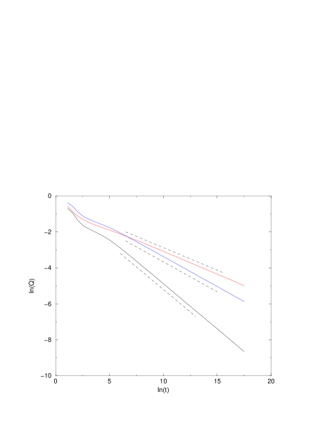
FIG. 3.: Double logarithmic plot of the survival probability $Q$ against time $t$ for the band model, for different types of absorbing boundary. The dashed lines with slope $-1/4$, $-1/3$ and $-1/2$ are guides to the eye. In order of increasing steepness, the corresponding data refer to absorbing boundaries given by (i) the negative $y$-axis, (ii) the negative $y$-axis and the negative $x$-axis and (iii) the whole $y$-axis. Least squares fits to the data give slopes -0.254, -0.333 and -0.501 respectively, consistent with the predicted values.

It is straightforward to apply the same general reasoning to the band model where the positive- and negative-flow bands are inequivalent. Consider a model where bands of width $b_{+}$ and $f(y)=v_{+}$ alternate with bands of width $b_{-}$ and $f(y)=-v_{-}$. For the special cases where $b_{+}v_{+}=b_{-}v_{-}$ there will be no macroscopic flow, and a coarse-grained description will lead to an anisotropic diffusion model as before, with the same values of $\theta$, e.g. $\theta=1/2$ if the whole $y$-axis is absorbing (indeed, $\theta=1/2$ will hold for any periodic $f(y)$ with zero mean). If $b_{+}v_{+}-b_{-}v_{-}>0$, the coarse-grained model has a mean flow away from the absorbing boundary, and the infinite-time survival probability is non-zero, while for $b_{+}v_{+}-b_{-}v_{-}<0$ the mean flow is towards the boundary and the survival probability decays exponentially with time. In the following subsection we provide an exact solution for the case $b_{+}v_{+}=b_{-}v_{-}$, in the limit $b_{-}\to 0$, $v_{-}\to\infty$, with $u=b_{-}v_{-}$ held fixed.

C A solvable model

The model we study is defined by a periodic function $f(y)$, with period $b$, given by

$$f(y)=v-u\,\delta(y),\ \ \ \ -b/2\leq y\leq b/2,$$ (30)

with $f(y+b)=f(y)$ for all $y$. The marginal case of interest, corresponding to no net flow, is given by $u=bv$. It is convenient, in the first instance, to compute the killing probability $P(x,y,t)$. The periodicity implies that we need only consider the regime $-b/2\leq y\leq b/2$, with the boundary conditions $\partial_{y}P(x,b/2,t)=\partial_{y}P(x,-b/2,t)=0$. The function $P$ obeys the BFPE

$$\partial_{t}P=D\partial_{yy}P+[v-u\delta(y)]\partial_{x}P.$$ (31)

Taking the Laplace transform with respect to time, and exploiting the initial condition $P(x,y,0)=1$ for all $x>0$, gives

$$D\partial_{yy}\tilde{P}+[v-u\delta(y)]\partial_{x}\tilde{P}-s\tilde{P}=0,$$ (32)

where $\tilde{P}(x,y,s)=\int_{0}^{\infty}dt\,\exp(-st)P(x,y,t)$. The general solution satisfying the given boundary conditions at $y=\pm b/2$ is (setting $D=1$ for convenience)

$$\tilde{P}(x,y,s) = \int_{0}^{\infty}dk\,a(k,s)e^{-kx}$$ (34)

$$\hskip 28.45274pt\times\cosh\left[\sqrt{kv+s}\,\left(\frac{b}{2}-|y|\right)\right],$$

for $y\neq 0$. Imposing the discontinuity in $\partial_{y}\tilde{P}$ at $y=0$ implied by Eq. (32), $\partial_{y}\tilde{P}(x,0+,s)-\partial_{y}\tilde{P}(x,0-,s)=u\partial_{x}\tilde{P}(x,0,s)$ for all $x>0$ and all $s$, leads to the condition

$$\tanh\gamma=\frac{ub}{\gamma v}\left(\frac{\gamma^{2}}{b^{2}}-\frac{s}{4}\right),$$ (35)

where

$$\gamma=\frac{b}{2}\sqrt{kv+s}.$$ (36)

Eq. (35) shows that only a single value of $k$ is possible for each $s$. Specialising to the marginal case $u=bv$, this equation simplifies to

$$\tanh\gamma=\gamma-\frac{b^{2}s}{4\gamma}\ .$$ (37)

The large-time behavior is governed by the small-$s$ solution of Eq. (37): $\gamma\simeq(3b^{2}s/4)^{1/4}$. Inserting this into Eq. (36) gives, for small $s$, $k\simeq 2\sqrt{3s}/bv$ and $\sqrt{kv+s}\simeq(3s)^{1/4}\sqrt{2/b}$. Putting these results into Eq. (34) gives

$$\tilde{P}(x,y,s) = a(s)\,\exp\left(-\frac{2\sqrt{3s}}{bv}\,x\right)$$ (39)

$$\hskip 28.45274pt\times\cosh\left(\frac{(3s)^{1/4}}{\sqrt{b/2}}\left(\frac{b}{2}-|y|\right)\right),$$

for $s\to 0$.

The amplitude $a(s)$ is fixed by the boundary condition, $P(0,0,t)=1$ for all $t$, which gives $\tilde{P}(0,0,s)=1/s$ and $a(s)=\{s\cosh[(3s)^{1/4}\sqrt{b/2}]\}^{-1}$ for small $s$. Since $Q(x,y,t)=1-P(x,y,t)$, we have $\tilde{Q}(x,y,s)=1/s-\tilde{P}(x,y,s)$. The small-$s$ result for $\tilde{P}$ determines the large-$t$ form of $Q(x,y,t)$ as

$$Q(x,y,t)=\frac{2\sqrt{3}}{b\sqrt{\pi t}}\,\left(\frac{x}{v}+\frac{1}{2}\,|y|(b-|y|)\right),$$ (40)

for $|y|\leq b/2$. This result confirms, for this special case, the result $Q(t)\sim t^{-1/2}$ obtained above using general heuristic arguments for the case where there is no net flow. Note that Eq. (40) has the same form as Eq. (28), and that this form holds for all values of $x/l$, where $l=vb^{2}/D$, i.e.  there is no analogue, in this model, of Eq.  (29) for $x\gg l$. This is because in the present model there is no regime in which the systems resembles a two-band model.

IV Discussion and Summary

In this paper we have obtained further results on the first-passage properties of a particle diffusing in the $y$-direction and subject to a deterministic drift velocity, $f(y)$, in the $x$-direction, with an absorbing boundary at $x=0$.

In the first part of the paper we considered the case where $f(y)\propto y^{\alpha_{+}}$ for $y>0$ and $f(y)\propto-|y|^{\alpha_{-}}$ for $y<0$. We confirmed the conjecture proposed in [1] that the larger power is ‘strongly dominating’ (in contrast to the ‘weakly dominating’ behaviour obtained when the exponents $\alpha_{+}$ and $\alpha_{-}$ are equal but the amplitudes are different [1]). We showed explicitly that for $\alpha_{+}>\alpha_{-}$ the survival probability approaches a non-zero limiting value, and we obtained an expression for this value.

In the second part of the paper we considered the case where $f(y)$ has a banded periodic form, with alternating bands of equal and opposite drift velocity. We presented numerical data, supported by a heuristic argument, to show that the asymptotic persistence exponent is $\theta=1/2$ in this case, and obtained a generalisation for different forms of absorbing boundary. We argued that the result generalises to any model where the coarse-grained flow field vanishes, and exemplified this result through a soluble model.

PG’s work was supported by EPSRC.

REFERENCES

- [1] A. J. Bray and P. Gonos, J. Phys. A 37, L361 (2004).
- [2] S. Redner and P. L. Krapivsky, J. Stat. Phys. 82, 999 (1996).
- [3] T. W. Burkhardt, J. Phys. A 33, L429 (2000).
- [4] S. Redner, A Guide to First-Passage Processes (CUP, Cambridge, 2001).
- [5] S. N. Majumdar, Curr. Sci. India 77, 370 (1999).
- [6] E. Sparre Andersen, Math. Scand. 1, 263 (1953); ibid. 2, 195 (1953).
- [7] M. E. Fisher and M. P. Gelfand, J. Stat. Phys. 53, 175 (1988).