Two stories outside Boltzmann-Gibbs statistics: Mori’s $q$-phase transitions and glassy dynamics at the onset of chaos

Abstract

First, we analyze trajectories inside the Feigenbaum attractor and obtain the atypical weak sensitivity to initial conditions and loss of information associated to their dynamics. We identify the Mori singularities in its Lyapunov spectrum with the appearance of a special value for the entropic index $q$ of the Tsallis statistics. Secondly, the dynamics of iterates at the noise-perturbed transition to chaos is shown to exhibit the characteristic elements of the glass transition, e.g. two-step relaxation, aging, subdiffusion and arrest. The properties of the bifurcation gap induced by the noise are seen to be comparable to those of a supercooled liquid above a glass transition temperature.

Key words: Edge of chaos, $q$-phase transitions, nonextensive statistics, external noise, glassy dynamics PACS: 05.45.Ac, 64.60.Ak, 05.40.Ca, 64.70.Pf

1 Introduction

Evidence for the incidence of nonextensive dynamical properties at critical attractors in low dimensional nonlinear maps has accumulated and advanced over the last few years; specially with regards to the onset of chaos in logistic maps - the Feigenbaum attractor [1, 7], and at the accompanying pitchfork and tangent bifurcations [8, 9]. The more general chaotic attractors with positive Lyapunov coefficients have full-grown phase-space ergodic and mixing properties, and their dynamics is compatible with the Boltzmann-Gibbs (BG) statistics. As a difference, critical attractors have vanishing Lyapunov coefficients, exhibit memory-retentive nonmixing properties, and are therefore to be considered outside BG statistics.

Naturally, some basic questions about the understanding of the dynamics at critical attractors are of current interest. We mention the following: Why do the anomalous sensitivity to initial conditions $\xi_{t}$ and its matching Pesin identity obey the expressions suggested by the nonextensive formalism? How does the value of the entropic index $q$ arise? Or is there a preferred set of $q$ values? Does this index, or indexes, point to some specific observable properties at the critical attractor?

From a broader point of view it is of interest to know if the anomalous dynamics found for critical attractors bears some correlation with the dynamical behavior at extremal or transitional states in systems with many degrees of freedom. Two specific suggestions have been recently advanced, in one case the dynamics at the onset of chaos has been demonstrated to be closely analogous to the glassy dynamics observed in supercooled molecular liquids [10], and in the second case the dynamics at the tangent bifurcation has been shown to be related to that at thermal critical states [11].

With regard to the above comments here we briefly recount the following developments:

i) The finding [7] that the dynamics at the onset of chaos is made up of an infinite family of Mori’s $q$-phase transitions [12, 13], each associated to orbits that have common starting and finishing positions located at specific regions of the attractor. Every one of these transitions is related to a discontinuity in the $\sigma$ function of ’diameter ratios’ [14], and this in turn implies a $q$ -exponential $\xi_{t}$ and a spectrum of $q$-Lyapunov coefficients equal to the Tsallis rate of entropy production for each set of attractor regions. The transitions come in pairs with conjugate indexes $q$ and $Q=2-q$, as these correspond to switching starting and finishing orbital positions. The amplitude of the discontinuities in $\sigma$ diminishes rapidly and consideration only of its dominant one, associated to the most crowded and sparse regions of the attractor, provides a very reasonable description of the dynamics, consistent with that found in earlier studies [1, 4].

ii) The realization [10] that the dynamics at the noise-perturbed edge of chaos in logistic maps is analogous to that observed in supercooled liquids close to vitrification. Four major features of glassy dynamics in structural glass formers, two-step relaxation, aging, a relationship between relaxation time and configurational entropy, and evolution from diffusive to subdiffusive behavior and finally arrest, are shown to be displayed by the properties of orbits with vanishing Lyapunov coefficient. The previously known properties in control-parameter space of the noise-induced bifurcation gap [14, 15] play a central role in determining the characteristics of dynamical relaxation at the chaos threshold.

2 Mori’s $q$-phase transitions at onset of chaos

The dynamics at the chaos threshold $\mu=\mu_{c}$ of the $z$-logistic map

$$f_{\mu}(x)=1-\mu\left|x\right|^{z},\;z>1,-1\leq x\leq 1,$$ (1)

has been analyzed recently [3, 7]. The orbit with initial condition $x_{0}=0$ (or equivalently, $x_{0}=1$) consists of positions ordered as intertwined power laws that asymptotically reproduce the entire period-doubling cascade that occurs for $\mu<\mu_{c}$. This orbit is the last of the so-called ’superstable’ periodic orbits at $\overline{\mu}_{n}<$ $\mu_{c}$, $n=1,2,...$ [14], a superstable orbit of period $2^{\infty}$. There, the ordinary Lyapunov coefficient $\lambda_{1}$ vanishes and instead a spectrum of $q$-Lyapunov coefficients $\lambda_{q}^{(k)}$ develops. This spectrum originally studied in Refs. [13] when $z=2$, has been shown [4, 7] to be associated to a sensitivity to initial conditions $\xi_{t}$ (defined as $\xi_{t}(x_{0})\equiv\lim_{\Delta x_{0}\to 0}(\Delta x_{t}/\Delta x_{0})$ where $\Delta x_{0}$ is the initial separation of two orbits and $\Delta x_{t}$ that at time $t$) that obeys the $q$-exponential form

$$\xi_{t}(x_{0})=\exp_{q}[\lambda_{q}(x_{0})t]\equiv[1-(q-1)\lambda_{q}(x_{0})\ t]^{-1/q-1}$$ (2)

suggested by the Tsallis statistics. Notably, the appearance of a specific value for the $q$ index (and actually also that for its conjugate value $Q=2-q$) works out [7] to be due to the occurrence of Mori’s ’$q$-phase transitions’ [12] between ’local attractor structures’ at $\mu_{c}$.

Figure 1: Absolute values of positions in logarithmic scales of iterations $\tau$ for a trajectory at

$\mu_{c}$ with initial condition $x_{0}=0$. The numbers correspond to iteration times.

As shown in Fig. 1, the absolute values for the positions $x_{\tau}$ of the trajectory with $x_{t=0}=0$ at time-shifted $\tau=t+1$ have a structure consisting of subsequences with a common power-law decay of the form $\tau^{-1/1-q}$ with $q=1-\ln 2/(z-1)\ln\alpha(z)$ [3], where $\alpha(z)$ is the Feigenbaum universal constant that measures the period-doubling amplification of iterate positions. That is, the attractor can be decomposed into position subsequences generated by the time subsequences $\tau=(2k+1)2^{n}$, each obtained by proceeding through $n=0,1,2,...$ for a fixed value of $k=0,1,2,...$. See Fig. 1. The $k=0$ subsequence can be written as $x_{t}=\exp_{2-q}(-\lambda_{q}^{(0)}t)$ with $\lambda_{q}^{(0)}=(z-1)\ln\alpha(z)/\ln 2$.

$q$-Lyapunov coefficients. The sensitivity $\xi_{t}(x_{0})$ can be obtained [7] from $\xi_{t}(m)\simeq\left|\sigma_{n}(m-1)/\sigma_{n}(m)\right|^{n}$, $t=2^{n}-1$, $n\$large, where $\sigma_{n}(m)=d_{n+1,m}/d_{n,m}$ and where $d_{n,m}$ are the diameters that measure adjacent position distances that form the period-doubling cascade sequence [14]. Above, the choices $\Delta x_{0}=d_{n,m}$ and $\Delta x_{t}=d_{n,m+t}$, $t=2^{n}-1$, have been made for the initial and the final separation of the trajectories, respectively. In the large $n$ limit $\sigma_{n}(m)$ develops discontinuities at each rational $m/2^{n+1}$ [14], and according to our expression for $\xi_{t}(m)$ the sensitivity is determined by these discontinuities. For each discontinuity of $\sigma_{n}(m)$ the sensitivity can be written in the forms $\xi_{t}=\exp_{q}[\lambda_{q}t]$ and $\xi_{t}=\exp_{2-q}[\lambda_{2-q}t]$, $\lambda_{q}>0$ and $\lambda_{2-q}<0$ [7]. This result reflects the multi-region nature of the multifractal attractor and the memory retention of these regions in the dynamics. The pair of $q$-exponentials correspond to a departing position in one region and arrival at a different region and vice versa, the trajectories expand in one sense and contract in the other. The largest discontinuity of $\sigma_{n}(m)$ at $m=0$ is associated to trajectories that start and finish at the most crowded ($x\simeq 1$) and the most sparse ($x\simeq 0$) regions of the attractor. In this case one obtains

$$\lambda_{q}^{(k)}=\frac{(z-1)\ln\alpha(z)}{(2k+1)\ln 2}>0,\ k=0,1,2,...,$$ (3)

the positive branch of the Lyapunov spectrum, when the trajectories start at $x\simeq 1$ and finish at $x\simeq 0$. By inverting the situation one obtains

$$\lambda_{Q}^{(k)}=-\frac{2(z-1)\ln\alpha(z)}{(2k+1)\ln 2}<0,\ k=0,1,2,...,$$ (4)

the negative branch of the Lyapunov spectrum. Notice that $\exp_{2-q}(y)=1/\exp_{q}(-y)$. So, when considering these two dominant families of orbits all the $q$-Lyapunov coefficients appear associated to only two specific values of the Tsallis index, $q$ and $Q=2-q$.

Mori’s $q$-phase transitions. As a function of the running variable $-\infty<{\sf q}<\infty$ the $q$-Lyapunov coefficients become a function $\lambda({\sf q})$ with two steps located at ${\sf q}=q=1-\ln 2/(z-1)\ln\alpha(z)$ and ${\sf q}=Q=2-q$. In this manner contact can be established with the formalism developed by Mori and coworkers [12] and the $q$-phase transition obtained in Refs. [13]. The step function for $\lambda({\sf q})$ can be integrated to obtain the spectrum $\phi({\sf q})$ ($\lambda({\sf q})\equiv d\phi/d\lambda({\sf q})$) and its Legendre transform $\psi(\lambda)$ ($\equiv\phi-(1-{\sf q})\lambda$), the dynamic counterparts of the Renyi dimensions $D({\sf q})$ and the spectrum $f(\widetilde{\alpha})$ that characterize the geometry of the attractor. The result for $\psi(\lambda)$ is

$$\psi(\lambda)=\left\{\begin{array}[]{l}(1-Q)\lambda,\ \lambda_{Q}^{(0)}<\lambda<0,\\ (1-q)\lambda,\ 0<\lambda<\lambda_{q}^{(0)}.\end{array}\right.$$ (5)

As with ordinary thermal 1st order phase transitions, a ”$q$-phase” transition is indicated by a section of linear slope $m=1-q$ in the spectrum (free energy) $\psi(\lambda)$, a discontinuity at $q$ in the Lyapunov function (order parameter) $\lambda({\sf q})$, and a divergence at $q$ in the variance (susceptibility) $v({\sf q})$. For the onset of chaos at $\mu_{c}(z=2)$ a $q$-phase transition was numerically determined [12, 13]. According to $\psi(\lambda)$ above we obtain a conjugate pair of $q$-phase transitions that correspond to trajectories linking two regions of the attractor, the most crowded and most sparse. See Fig. 2. Details appear in Ref. [7].

Figure 2: $q$-phase transitions with index values $q=0.2445$ and $Q=2-q=1.7555$ obtained for $z=2$ from the main discontinuity in $\sigma_{n}(m)$. See text for details.

Generalized Pesin identity. Ensembles of trajectories with starting points close to the attractor point $x_{0}$ expand in such a way that a uniform distribution of initial conditions remains uniform for all later times $t$. As a consequence of this we established [4, 7] the identity of the rate of entropy production $K_{q}^{(k)}$ with $\lambda_{q}^{(k)}$. The $q$-generalized rate of entropy production $K_{q}$ is defined via $K_{q}t=S_{q}(t)-S_{q}(0)$, $t$ large, where

$$S_{q}\equiv\sum_{i}p_{i}\ln_{q}\left(\frac{1}{p_{i}}\right)=\frac{1-\sum_{i}^{W}p_{i}^{q}}{q-1}$$ (6)

is the Tsallis entropy, $p_{i}$ is the trajectories’ distribution, and where $\ln_{q}y\equiv(y^{1-q}-1)/(1-q)$ is the inverse of $\exp_{q}(y)$. See Figs. 2 and 3 in Ref. [4].

3 Glassy dynamics at noise-perturbed onset of chaos

We describe now the effect of additive noise in the dynamics at the onset of chaos. The logistic map $z$ $=2$ reads now

$$x_{t+1}=f_{\mu}(x_{t})=1-\mu x_{t}^{2}+\chi_{t}\sigma,\ -1\leq x_{t}\leq 1,\ 0\leq\mu\leq 2,$$ (7)

where $\chi_{t}$ is Gaussian-distributed with average $\left\langle\chi_{t}\chi_{t^{\prime}}\right\rangle=\delta_{t.t^{\prime}}$, and $\sigma$ is the noise intensity. For $\sigma>0$ the noise fluctuations wipe the fine features of the periodic attractors as these widen into bands similar to those in the chaotic attractors, nevertheless there remains a well-defined transition to chaos at $\mu_{c}(\sigma)$ where the Lyapunov exponent $\lambda_{1}$ changes sign. The period doubling of bands ends at a finite maximum period $2^{N(\sigma)}$ as $\mu\rightarrow\mu_{c}(\sigma)$ and then decreases at the other side of the transition. This effect displays scaling features and is referred to as the bifurcation gap [14, 15]. When $\sigma>0$ the trajectories visit sequentially a set of $2^{n}$ disjoint bands or segments leading to a cycle, but the behavior inside each band is fully chaotic. These trajectories represent ergodic states as the accessible positions have a fractal dimension equal to the dimension of phase space. When $\sigma=0$ the trajectories correspond to a nonergodic state, since as $t\rightarrow\infty$ the positions form only a Cantor set of fractal dimension $d_{f}=0.5338...$. Thus the removal of the noise $\sigma\rightarrow 0$ leads to an ergodic to nonergodic transition in the map.

As shown in Ref. [10] when $\mu_{c}(\sigma>0)$ there is a ’crossover’ or ’relaxation’ time $\tau_{x}=\sigma^{r-1}$, $r\simeq 0.6332$, between two different time evolution regimes. This crossover occurs when the noise fluctuations begin suppressing the fine structure of the attractor as displayed by the superstable orbit with $x_{0}=0$ described previously. For $\tau<\tau_{x}$ the fluctuations are smaller than the distances between the neighboring subsequence positions of the $x_{0}=0$ orbit at $\mu_{c}(0)$, and the iterate position with $\sigma>0$ falls within a small band around the $\sigma=0$ position for that $\tau$. The bands for successive times do not overlap. Time evolution follows a subsequence pattern close to that in the noiseless case. When $\tau\sim\tau_{x}$ the width of the noise-generated band reached at time $\tau_{x}=2^{N(\sigma)}$ matches the distance between adjacent positions, and this implies a cutoff in the progress along the position subsequences. At longer times $\tau>\tau_{x}$ the orbits no longer trace the precise period-doubling structure of the attractor. The iterates now follow increasingly chaotic trajectories as bands merge with time. This is the dynamical image - observed along the time evolution for the orbits of a single state $\mu_{c}(\sigma)$ - of the static bifurcation gap initially described in terms of the variation of the control parameter $\mu$ [15].

Two-step relaxation. Amongst the main dynamical properties displayed by supercooled liquids on approach to glass formation is the growth of a plateau, and for that reason a two-step process of relaxation, in the time evolution of two-time correlations [16].

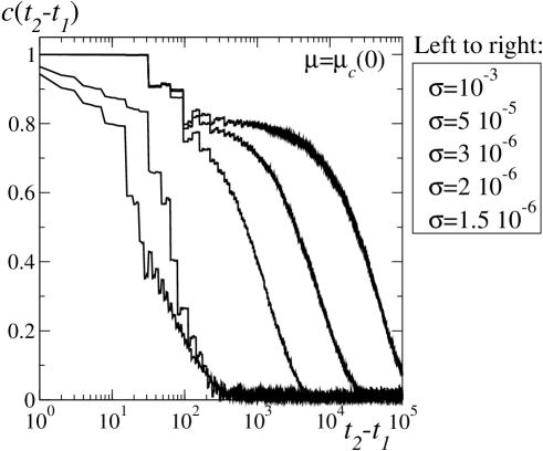
Figure 3: Two-time correlation function $c(t_{2}-t_{1})$ for an ensemble of trajectories with $x_{0}=0$ for different values of noise amplitude $\sigma$. See text for details.

This consists of a primary power-law decay in time difference $\Delta t$ (so-called $\beta$ relaxation) that leads into the plateau, the duration $t_{x}=\tau_{x}-1$ of which diverges also as a power law of the difference $T-T_{g}$ as the temperature $T$ decreases to a glass temperature $T_{g}$. After $t_{x}$ there is a secondary power law decay (so-called $\alpha$ relaxation) away from the plateau [16]. In Fig. 3 we show [17] the behavior of the correlation function

$$c(t_{2}-t_{1})=\frac{\left\langle x_{t_{2}}x_{t_{1}}\right\rangle-\left\langle x_{t_{2}}\right\rangle\left\langle x_{t_{1}}\right\rangle}{\chi_{t_{1}}\chi_{t_{2}}},$$ (8)

for different values of noise amplitude. Above, $\left\langle...\right\rangle$ represents an average over an ensemble of trajectories starting at $x_{0}=0$ and $\chi_{t_{i}}=\sqrt{\left\langle x_{t_{i}}^{2}\right\rangle-\left\langle x_{t_{i}}\right\rangle^{2}}$. The development of the two power-law relaxation regimes and their intermediate plateau can be clearly appreciated. See Ref. [10] for the interpretation of the map analogs of the $\alpha$ and $\beta$ relaxation processes.

Aging scaling. A second important (nonequilibrium) dynamical property of glasses is the loss of time translation invariance observed for $T\leq T_{g}$, a characteristic known as aging. The drop time of relaxation functions and correlations display a scaling dependence on the ratio $t/t_{w}$ where $t_{w}$ is a waiting time. In Fig. 4a we show [17] the correlation function

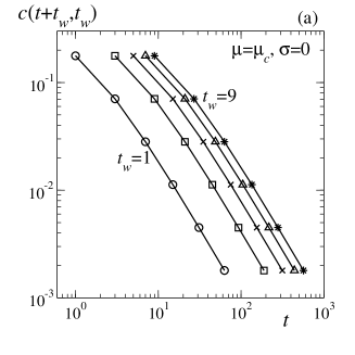
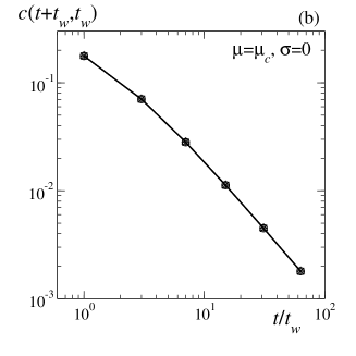
Figure 4: a) Two-time correlation function

$c(t+t_{w},t_{w})$ for different values of $\sigma$. b) The same data in terms of the rescaled variable $t/t_{w}.$ See text for details.]

$$c(t+t_{w},t_{w})=(1/N)\sum_{j=1}^{N}x_{(t+t_{w})j}x_{tj}$$ (9)

for different values of $\sigma$, and in Fig. 4b the same data where the rescaled variable $t/t_{w}=2^{n}-1$, $t_{w}=2k+1$, $k=0,1,...$, has been used. The characteristic aging scaling behavior is patent. See Ref. [10] for an analytical description of the built-in aging properties of the trajectories at $\mu_{c}(\sigma)$.

Adam-Gibbs relation. A third notable property is that the experimentally observed relaxation behavior of supercooled liquids is well described, via standard heat capacity assumptions [16], by the so-called Adam-Gibbs equation, $t_{x}=A\exp(B/TS_{c})$, where $t_{x}$ is the relaxation time at $T$, and the configurational entropy $S_{c}$ is related to the number of minima of the fluid’s potential energy surface [16]. See Ref. [10] for the derivation of the analog expression for the nonlinear map. Instead of the exponential Adam-Gibbs equation, this expression turned out to have the power law form

$$t_{x}=(s/S_{c})^{(1-r)/r}.$$ (10)

Since $(1-r)/r\simeq 0.5792$ then $t_{x}\rightarrow\infty$ and $S_{c}\rightarrow 0$ as $\sigma\rightarrow 0$.

Subdiffusion and arrest. A fourth distinctive property of supercooled liquids on approach to vitrification is the progression from normal diffusivity to subdiffusive behavior and finally to a halt in the growth of the molecular mean square displacement.

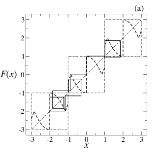
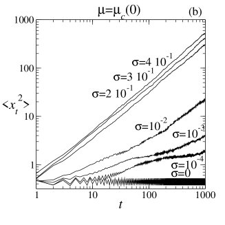
Figure 5: a) Repeated-cell map and trajectory. b) Mean square displacement $\left\langle x_{t}^{2}\right\rangle$ for trajectories with $x_{0}=0$ for several values of noise amplitude $\sigma$. See text for details.

To investigate this aspect of vitrification in the map at $\mu_{c}(\sigma)$, we constructed [17] a periodic map with repeated cells of the form $x_{t+1}=F(x_{t})$, $F(l+x)=l+F(x)$, $l=...-1,0,1,...$, $F(-x)=F(x)$, where

$$F(x)=\left\{\begin{array}[]{c}-\left|1-\mu_{c}x^{2}\right|+\chi\sigma,\;-1\leq x<0,\\ \left|1-\mu_{c}x^{2}\right|+\chi\sigma,\;0\leq x<1.\end{array}\right.$$ (11)

Fig. 5a shows this map together with a portion of one of its trajectories, while Fig. 5b shows the mean square displacement $\left\langle x_{t}^{2}\right\rangle$ as obtained from an ensemble of trajectories with $x_{0}=0$ for several values of noise amplitude. The progression from normal diffusion to subdiffusion and to final arrest can be plainly observed as $\sigma\rightarrow 0$ [17].

4 Summary

We reviewed recent understanding on the dynamics at the onset of chaos in the logistic map. We exhibited links between previous developments, such as Feigenbaum’s $\sigma$ function, Mori’s $q$-phase transitions and the noise-induced bifurcation gap, with more recent advances, such as $q$-exponential sensitivity to initial conditions [3, 5], $q$-generalized Pesin identity [4, 7] and dynamics of glass formation [10].

An important finding is that the dynamics is constituted by an infinite family of Mori’s $q$-phase transitions, each associated to orbits that have common starting and finishing positions located at specific regions of the attractor. Thus, the special values for the Tsallis entropic index $q$ in $\xi_{t}$ and $S_{q}$ are equal to the special values of the variable $q$ at which the $q$-phase transitions take place.

As described, the dynamics of noise-perturbed logistic maps at the chaos threshold presents the characteristic features of glassy dynamics observed in supercooled liquids. The limit of vanishing noise amplitude $\sigma\rightarrow 0$ (the counterpart of the limit $T-T_{g}\rightarrow 0$ in the supercooled liquid) leads to loss of ergodicity. This nonergodic state with $\lambda_{1}=0$ corresponds to the limiting state, $\sigma\rightarrow 0$, $t_{x}\rightarrow\infty$, of a family of small $\sigma$ states with glassy properties, which are expressed for $t<t_{x}$ via the $q$-exponentials of the Tsallis formalism.

Acknowledgments. FB warmly acknowledges hospitality at UNAM where part of this work has been done. Work partially supported by DGAPA-UNAM and CONACyT (Mexican Agencies).

References

- [1] C. Tsallis, A.R. Plastino and W.-M. Zheng, Chaos, Solitons and Fractals 8, 885 (1997).
- [2] M.L. Lyra and C. Tsallis, Phys. Rev. Lett. 80, 53 (1998).
- [3] F. Baldovin and A. Robledo, Phys. Rev. E 66, 045104 (2002).
- [4] F. Baldovin and A. Robledo, Phys. Rev. E 69, 045202 (2004).
- [5] E. Mayoral and A. Robledo, Physica A 340, 219 (2004).
- [6] G.F.J. Añaños and C. Tsallis, Phys. Rev. Lett. 93, 020601 (2004).
- [7] E. Mayoral and A. Robledo, submitted and cond-mat/0501366.
- [8] A. Robledo, Physica A 314, 437 (2002); Physica D 193, 153 (2004).
- [9] F. Baldovin and A. Robledo, Europhys. Lett. 60, 518 (2002).
- [10] A. Robledo, Phys. Lett. A 328, 467 (2004); Physica A 342, 104 (2004).
- [11] A. Robledo, Physica A 344, 631 (2004).
- [12] H. Mori, H. Hata, T. Horita and T. Kobayashi, Prog. Theor. Phys. Suppl. 99, 1 (1989).
- [13] H. Hata, T. Horita and H. Mori, Progr. Theor. Phys. 82, 897 (1989); G. Anania and A. Politi, Europhys. Lett. 7 (1988).
- [14] See. for example, H.G. Schuster, Deterministic Chaos. An Introduction, 2nd Revised Edition (VCH Publishers, Weinheim, 1988).
- [15] J.P. Crutchfield, J.D. Farmer and B.A. Huberman, Phys. Rep. 92, 45 (1982).
- [16] For a review see, P.G. De Benedetti and F.H. Stillinger, Nature 410, 267 (2001).
- [17] F. Baldovin and A. Robledo, to be submitted.