Statistical properties of fracture in a random spring model
Abstract
Using large scale numerical simulations we analyze the statistical properties of fracture in the two dimensional random spring model and compare it with its scalar counterpart: the random fuse model. We first consider the process of crack localization measuring the evolution of damage as the external load is raised. We find that, as in the fuse model, damage is initially uniform and localizes at peak load. Scaling laws for the damage density, fracture strength and avalanche distributions follow with slight variations the behavior observed in the random fuse model. We thus conclude that scalar models provide a faithful representation of the fracture properties of disordered systems.
I introduction
The statistical properties of fracture in disordered media represent an intriguing theoretical problem with important practical applications breakdown . The presence of disorder naturally leads to statistical distributions of failure stresses, accumulated damage, acoustic activity, crack shapes and so on. The application of a standard continuum descriprion based on elastic equation cannot capture the effect of fluctuations and hence the effect of disorder has to be considered explicitly. A well established way to deal with this problem relies on lattice models, in which the medium is described by a discrete set of elastic bonds with randomly distributed failure thresholds breakdown . In the simplest approximation of a scalar displacement, one recovers the random fuse model (RFM) where a lattice of fuses with random thresholds are subject to an increasing external current deArcangelis85 .
The RFM has been extensively investigated in the last twenty years, mainly using numerical simulations breakdown ; deArcangelis85 ; kahng88 ; deArcangelis89 ; delaplace ; zrvs ; hansen001 ; nukalajpamg . The type of behavior at macroscopic fracture is significantly influenced by the amount of disorder kahng88 . When the disorder is narrowly distributed, materials breakdown without significant precursors. As the disorder increases, substantial damage is accumulated prior to failure and the dynamics resembles percolation sornette . Indeed, in the limit of infinite disorder, the damage accumulation process can exactly be mapped onto a percolation problem guyon88 . It has been suggested that for strong, but finite, disorder fracture should be interpreted as a first order transition near a spinodal point zrvs . In addition, the fracture of the RFM is preceded by avalanches of failure events zrvs ; hansen ; alava ; ZAP-05 . These are reminiscent of the acoustic emission activity observed in experiments and their distribution follows a power law. Finally, the RFM has also been used to compute the fracture strength distribution and the related size effects duxbury86 ; duxbury87 ; duxbury88 ; beale88 ; nukalaepjb .
Modeling the elastic medium using the RFM introduces drastic approximations in terms of the discretization process, quasistatic dynamics and the scalar nature of the interactions. It is thus important to clarify if the observations made in the RFM carry over to more complex and realistic situations. In this paper, we address the problem of the scalar (electric) interactions of the RFM, by comparing it with a tensorial central force model, the random spring model (RSM) sahimi86 . The model is a tensorial counterpart of the RFM: it has quasistatic dynamics, random thresholds, but fuses and currents are replaced by elastic springs and forces. Dynamic effects have been instead considered in Refs. minozzi ; politi .
After discussing the model in Sec. II, we consider the typical statistical measures performed using the RSM: damage localization and average damage profiles are reported in Sec. III, while mean damage scaling and damage distributions are discussed in Sec. IV. and Sec. V respectively. In Sec. VI and VII we discuss the fracture strenght distribution and the size effect on the mean strength. The avalanche behavior is analyzed in Sec. VII and a summary is reported in Sec VIII. We have not analyzed the roughness of the final crack since in several instances the spring networks fail because of loss of rigidity.
II The random spring model
In the RSM, the lattice is initially fully intact with bonds having the same stiffness, but the bond breaking thresholds, , are randomly distributed based on a thresholds probability distribution, . The bond breaks irreversibly, whenever the force in the spring exceeds the breaking threshold force value, , of the spring. Periodic boundary conditions are imposed in the horizontal direction and a constant unit displacement difference is applied between the top and the bottom of lattice system.
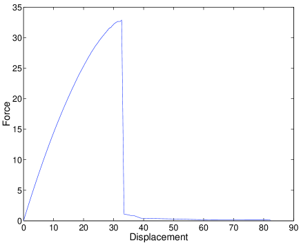
Numerically, a unit displacement, , is applied at the top of the lattice system and the equilibrium equations are solved to determine the force in each of the springs. Subsequently, for each bond , the ratio between the force and the breaking threshold is evaluated, and the bond having the largest value, , is irreversibly removed. The forces are redistributed instantaneously after a bond is broken implying that the stress relaxation in the lattice system is much faster than the breaking of a bond. Each time a bond is broken, it is necessary to re-equilibrate the lattice system in order to determine the subsequent breaking of a bond. The process of breaking of a bond, one at a time, is repeated until the lattice system falls apart. For the RSM, we consider a triangular lattice system network and a uniform probability distribution for thresholds disorder, which is constant between 0 and 1. The diamond lattice (square lattice with bonds inclined at 45 degrees) spring system exhibits certain unstable modes and hence is not considered. Figure 1 presents the envelope of a typical force-displacement response obtained using the RSM. The peak load of the lattice system is defined as the maximum force of the force-displacement response.
Numerical simulation of fracture using large lattice networks is often hampered due to the high computational cost associated with solving a new large set of linear equations every time a new lattice bond is broken. In this study, we use the multiple-rank sparse Cholesky factorization updating algorithm developed in Ref. nukalajpamg for simulating fracture using discrete lattice systems. In comparison with the Fourier accelerated iterative schemes used for modeling lattice breakdown bat-98 , this algorithm significantly reduced the computational time required for solving large lattice systems. Using this numerical algorithm, we were able to investigate damage evolution in large ( for spring model) initially fully intact discrete lattice systems. However, due to insufficient number of available sample configurations, in this paper, we consider results up to for spring models. For many lattice system sizes, the number of sample configurations, , used are excessively large to reduce the statistical error in the numerical results (see Table 1). In Table 1, the fraction of broken bonds (or damage density) for each of the lattice system sizes is obtained by dividing the number of broken bonds with the total number of bonds, , present in the fully intact lattice system. For triangular lattice topology, . The lattice system sizes considered in this work are . However, since corrections to the scaling laws are strongest for small lattice systems, in the following, we use lattice sizes for obtaining the scaling exponents. Table 1 presents mean and standard deviations in the broken bond density (fraction of broken bonds) at the peak load and at failure for various triangular lattice system sizes.
III Diffusive Damage and Localization
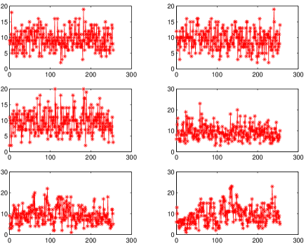
Qualitatively, damage evolution as described by breaking of bonds is controlled by two competing aspects: disorder and stress concentration in the vicinity of crack tips. In the case of strong disorder, bond breaking events occur in an uncorrelated manner in the initial stages of damage evolution and thus resemble percolation. As the damage starts to accumulate, some degree of correlation can be expected due to the presence of stress concentration at the crack tips. A natural question to ask concerns the relevance of these correlations as failure is approached. If correlations are irrelevant one should observe percolation scaling up to failure, as in the case of infinite disorder. On the other hand, in the weak disorder case, the current enhancement at the crack tips is so strong that a spanning crack is nucleated soon after a few bonds (or even a single bond) are broken kahng88 . The interesting situation corresponds to the diffuse damage and localization regime, where a substantial amount of damage is accumulated prior to failure. Figure 2 presents the snapshots of damage evolution in a typical RSM simulation of size .
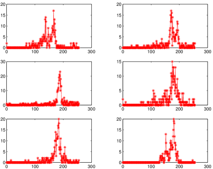
In order to investigate the localization of damage prior to failure, we divided the load-displacement response of a typical RSM simulation into 12 segments, with six equal segments each before and after the peak load. Figures 3 and 4 present the snapshots of damage profiles within each segment of load-displacement curve of a typical simulation with uniform threshold disorder for . Based on Figs. 3 and 4, it is clear that localization of damage occurs in the RSM prior to failure even for strong but finite disorder. In fact, the damage is diffusive in the initial stages of loading and extends upto almost the peak load. Around the peak load, the damage starts to localize and ultimately leads to failure, and hence the final breakdown event is very different from the initial precursors upto the peak load. Similar behavior is observed in the random thresholds fuse model with both uniform and power law thresholds distributions nukalajstat .
In order to obtain a quantitative description of the damage localization process it is necessary to average the damage profiles over different realizations. Since the localization of damage can occur anywhere along the direction of the lattice, a simple averaging of the damage profiles would yield a flat profile irrespective of the individual profile shapes in a single realization. In this study, we average the damage profiles by first shifting the damage profiles by the center of mass of the damage and then averaging. Alternatively, one could average the magnitude of the Fourier transforms of individual damage profiles thereby retaining the frequency content of damage profiles. The Fourier method eliminates any artificial biasing associated with the shifting of the individual profiles in the real-space nukalajstat .
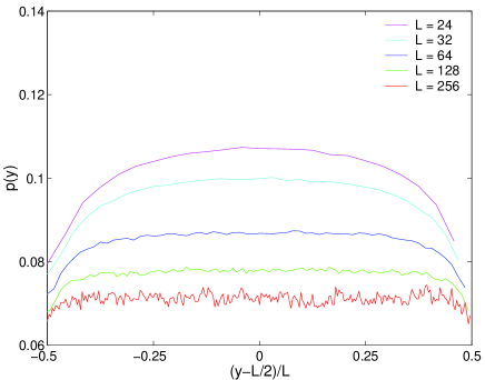
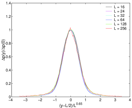
Figure 5 presents the average damage profiles for the damage accumulated up to the peak load by first shifting the damage profiles by the center of mass of the damage and then averaging over different samples. The results presented in Fig. 5 indicate that although the average damage profiles at smaller lattice system sizes are not completely flat, they flatten considerably as the lattice system size is increased. We tend thus to attribute the apparent profile to size effects. Indeed, for large system sizes (e.g. and ), the results clearly show that there is no localization at the peak load. Consequently, the localization of damage is mostly due to the damage accumulated between the peak load and failure, i.e., the final catastrophic breakdown event. Figure 6 presents the data collapse of the average damage profiles for the damage accumulated between the peak load and failure using a power law scaling. A perfect collapse of the data is obtained using the form
| (1) |
where the damage peak scales as and the localization length scales as , with (see Fig. 6). The profile shapes decay exponentially at large system sizes. We have also tried a simple linear scaling of the form , but the collapse of the data is not very good. The result for the fuse model is similar: the profile also displays exponential tails and the exponent is found to be .
IV Scaling of damage density
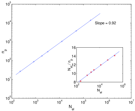
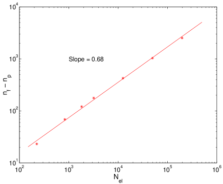
It has been noted in the previous section that the final breakdown event is very different from the initial precursors. Thus, we consider the scaling of the number of broken bonds at the peak load, , that excludes the last catastrophic event. In Fig. 7 we plot as a function of the lattice size . The data displays a reasonable power law behavior , with . The exponent is in close agreement with the value obtained for random thresholds fuse model using both triangular () and diamond () lattice topologies nukalajstat . The difference between the RSM and RFM models is marginal and may be attributed to the results obtained from the smaller lattice sizes, where corrections to the fractal scaling may exist. However, we have noticed some systematic deviations from the scaling form by plotting vs . Since the exponent is close to one, the data could be equally well fit by a linear law times a logarithmic correction as suggested in Ref. mikko04 (see the inset of Fig. 7). Both these fits imply that in the limit of large lattices the fraction of broken bonds prior to fracture vanishes.
V Scaling of Damage Density Probability Distributions
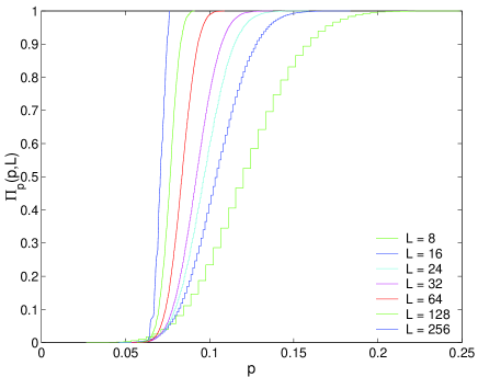
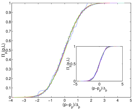
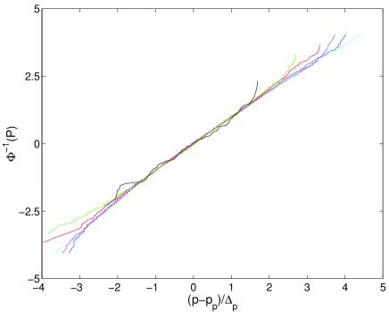
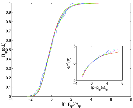
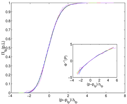
Since the final breakdown event is very different from the initial precursors up to the peak load, in this section, we present the scaling of the cumulative probability distributions for the fraction of broken bonds at the peak load. The cumulative probability distribution for the damage density at the peak load is defined as the probability that a system of size reaches peak load when the fraction of broken bonds equals , where is the number of broken bonds. Figure 8 presents the cumulative probability distribution for the damage density at the peak load in the random thresholds spring model for various system sizes . By simply plotting the distribution in terms of , where and denote the mean and standard deviation of the number of broken bonds at peak load, and and denote the mean and standard deviation of fraction of broken bonds at peak load (see Table 1), we obtain a very good collapse of the cumulative probability distribution of the damage density at the peak load. Fig. 9 shows that may be expressed in a universal scaling form such that for different system sizes . A similar collapse has been performed for the random thresholds fuse model in the Ref. nukalajstat . The inset in Fig. 9 presents the comparison of the cumulative damage density probability distributions in the random thresholds spring and fuse models. The excellent collapse of the data in the inset of Fig. 9 suggests that the cumulative probability distribution for the damage density at the peak load, , may be universal. Finally, the collapse of the data in Fig. 10 indicates that a Gaussian distribution adequately describes .
In Ref. nukalajstat , we have also checked that the distributions at failure in the random thresholds fuse model obey essentially the same laws, i.e., , where is the probability that a system of size fails when the fraction of broken bonds equals , and is the corresponding reduced variable at failure. However, in the RSM, although a reasonable collapse of the cumulative probability distribution of damage density at failure can be obtained, the cumulative distributions of damage density at peak load and at failure appear to be different. In particular, the distribution, , at failure is not adequately described by a Gaussian distribution. The inadequacy of a Gaussian distribution in the post-peak regime may indicate the presence of a relatively stronger localization in the RSM compared with the RFM.
VI Universality of fracture strength distribution
In this study, we start the numerical simulation with a fully intact lattice system. The fracture strength of such a system is defined as the stress corresponding to the peak load of the lattice system response.
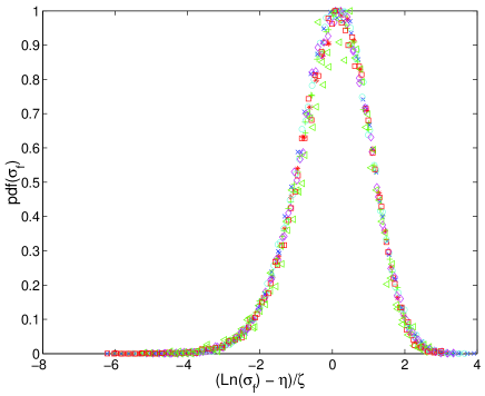
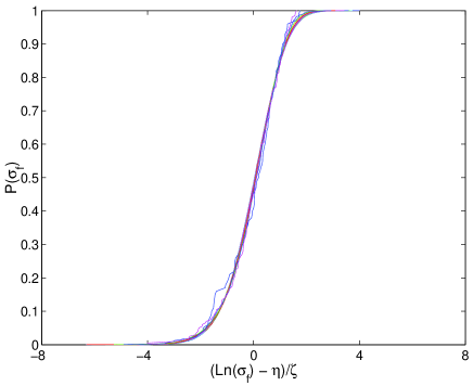
Figure 11(a) presents the fracture strength density distributions for random thresholds spring model using the standard Lognormal variable, , defined as , where refers to the fracture strength defined as the peak load divided by the system size , and and refer to the mean and the standard deviation of the logarithm of . In order to verify the universality of fracture strength distribution, the fracture strength distributions from nukalaepjb corresponding to random thresholds fuse model (RFM) using triangular lattice systems with uniform disorder are presented in Fig. 11(a) along with those corresponding to random thresholds spring model. In particular, Fig. 11(a) shows the data for different lattice system sizes, , corresponding to (a) triangular spring lattice, and (b) triangular fuse lattices of sizes . In all, there are 13 plots in Fig. 11(a), and the excellent collapse of the data for various spring and fuse lattices clearly indicates the universality of the fracture strength density distribution. The results presented in Fig. 11(a) are limited only up to a system size of due to the availability of fewer sample configurations for larger lattice systems. In order to attain a good collapse of the data for the density distributions, it is necessary to consider many sample configurations. On the other hand, good collapse of the data for the cumulative distributions can be achieved using fewer number of sample configurations. Figure. 11(b) presents the cumulative fracture strength versus the standard Lognormal variable, , for random spring and fuse lattice networks for system sizes up to . In particular, in Fig. 11(b), we plot the numerical simulation results of RSM for system sizes along with those of RFM for system sizes . In all, there are about 16 curves (7 for triangular spring lattices and 9 for triangular fuse lattices) in Fig. 11(b), and the excellent collapse of the data suggests universality of fracture strength distribution. In Ref. nukalaepjb , we have also presented the collapse of the fracture strength distribution for different lattice topologies (such as triangular and diamond), which is consistent with the notion of universality of fracture strength distribution. That is, , where refers to the cumulative probability of fracture strength , is a universal function such that , and is the standard Lognormal variable.
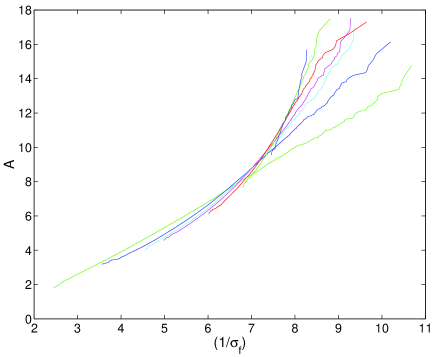
Figures 12(a) and 12(b) present the modified Gumbel and Weibull fits for the fracture strength distribution of triangular spring lattice network using
| (2) |
for the modified Gumbel distribution, and
| (3) |
for the Weibull distribution. In Eqs. 2 and 3, , , and are constants, and is defined as
| (4) |
where denotes the cumulative distribution. From these figures, it is clear that fracture strength data for different lattice system sizes does not collapse on to a single straight line as it should, if the data were to follow Eq. (2) or (3). This indicates that neither modified Gumbel nor Weibull distributions may represent the fracture strengths distribution accurately for the RSM. In the Ref. nukalaepjb , similar conclusion has been drawn for the fracture strengths distribution of RFM.
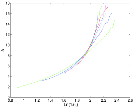
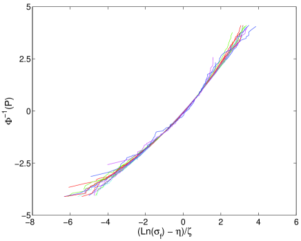
On the other hand, in Fig. 12(c), we test the Lognormal description for fracture strengths by plotting the inverse of the cumulative probability, , against the standard Lognormal variable, . In the above description, denotes the standard normal probability function. In particular, in the Fig. 12(c) we present the Lognormal fit for the cumulative fracture strength distributions obtained for random thresholds spring and fuse models (i.e., for all of the 16 curves in Fig. 11(b)). Once again, this figure clearly indicates that the fracture strength distribution obtained for different lattice system sizes collapses onto a single curve, albeit minute deviation from straight line behavior is evident. We have also used the normal distribution to collapse the fracture strength data of triangular spring and fuse lattice systems. Although the data collapse is reasonable, it is not as good as that of Lognormal distribution based on Kolmogorov-Smirnov goodness-of-fit test.
VII Size effects in the mean fracture strength
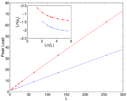
The mean fracture strength data for various random threshold spring lattice system sizes is presented in Table 2. In Ref. nukalaepjb , for the RFM, we have suggested a scaling form for the peak load, where and are constants. Correspondingly, the mean fracture strength defined as , is given by . We have used the same scaling law for the random thresholds spring model as well, and the result presented in Fig. 13 indicates that the exponent is approximately equal to , which is once again in consistent with the obtained for RFM using both triangular and diamond lattice topologies. The inset in Fig. 13 presents a power law fit that is consistent with a Weibull distribution for fracture strengths. From the nonlinearity of the plots in the inset of Fig. 13, it is clear that the mean fracture strength does not follow a simple power law scaling that is consistent with a Weibull distribution for fracture strengths. We have also verified that the mean fracture strength does not follow a scaling law of form that is consistent with a modified Gumbel distribution for fracture strengths duxbury86 ; duxbury87 ; duxbury88 ; beale88 .
Since a very small negative exponent is equivalent to a logarithmic correction, i.e., for , , an alternative expression for the mean fracture strength may be obtained as , where and are constants that are related to the constants and . This suggests that the mean fracture strength of the lattice system decreases very slowly with increasing lattice system size, and scales as , with , for very large lattice systems.
VIII Avalanches
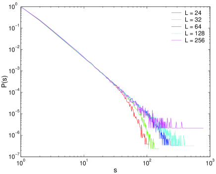
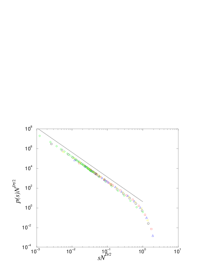
The avalanche size distribution, once the last event is excluded, is a power law followed by an exponential cutoff at large avalanche sizes (see Fig. 14) nota . The cutoff size is increasing with the lattice size, so that we can describe the distribution by a scaling form
| (5) |
where represents the fractal dimension of the avalanches and is the number of bonds. Figure 15 presents the data collapse of the distribution of avalanche sizes using the exponents and .
So far we have considered avalanche statistics integrating the distribution over all the values of the forces upto the peak load, but the avalanche signal is not stationary: as the force increases so does the avalanche size. In particular, the last avalanche is much larger than the others. Its typical size grows as , with (see Fig. 16), which is once again in good agreement with the value obtained for RFM (see Fig. 14 of Ref. nukalajstat ). The cumulative distribution of last avalanche sizes for the RSM and RFM is presented in Figs. 17(a) and (b) respectively. While the distribution is approximately Gaussian for RFM as shown by the data collapse (almost linear) in the inset of Fig. 17(b), there appears to be significant nonlinearity in the data collapse of the plots in the inset of Fig. 17(a). This suggests that normal distribution may not be an adequate fit for representing the distribution of last avalanche size in the RSM model. We notice here that the post-peak regime is different in the two models because the RSM can fail because of a loss in rigidity. In general, the significantly different nature of the last avalanche with respect to the precursors is revealed both by the distribution type (Gaussian or power law) and by its characteristic value, scaling as or . This difference reflects the fact that the last avalanche is a catastrophic event corresponding to unstable crack growth, while precursors reflect metastable crack growth and the two processes are different.
IX Summary
In this study we investigated the universality of random thresholds spring and fuse models using large scale numerical simulations and large number of sample configurations to reduce the statistical error in the numerical results. For both models, we considered triangular lattice topology with uniform disorder and increased the load quasistatically. We performed several statistical measures characterizing the fracture process that can be summarized as follows:
-
1.
Damage localization: the process of localization is similar in the RFM and RSM. Damage is accumulated in a uniform manner up to the peak load and then suddently localizes leading to complete failure. This process is described by damage profiles, that are basically flat until peak load and show a peak, with exponential tails, in the post peak regime. The collapse of the damage profiles implies some small differences in the exponets for the two models.
-
2.
Damage density: The number of broken bonds at failure or at peak load scales with the lattice size. We have shown that the behavior in RFM and RSM is very similar, but in both cases it is not possibile to distinguish a power law from a linear behavior with a logarithmic correction.
-
3.
Damage distributions: The distribution of broken bonds at peak load follows the normal distribution for RFM and RSM.
-
4.
Fracture strength: The fracture strength distribution is found to be lognormal for both models and the mean fracture strength scales logarithmically.
-
5.
Avalanches: The integrated avalanche distributions follow a power law in both models. The results of the RSM yields an exponent that is very close to the exponent observed in global load sharing fiber bundle model (FBM), while larger deviations are found in the RFM (i.e. ZAP-05 ).
Thus in conclusion, we can state that RFM and RSM are qualitatively very similar: distributions have the same forms, localization proceeds in the same way, avalanches are similar. The only diffirences can be found in small quantitative deviations in exponents. We can not rule out that these are due to differences in the finite size behavior of the models and that at large scales the behavior is the same. In addition, the rigidity mechanism present in the RSM and not in the RSM could explain some deviations in the post-peak regime.
Acknowledgment
This research is sponsored by the
Mathematical, Information and Computational Sciences Division, Office
of Advanced Scientific Computing Research, U.S. Department of Energy
under contract number DE-AC05-00OR22725 with UT-Battelle, LLC.
References
- (1) H. J. Herrmann and S. Roux (eds.), Statistical Models for the Fracture of Disordered Media, (North-Holland, Amsterdam, 1990). B. K. Chakrabarti and L. G. Benguigui, Statistical physics of fracture and breakdown in disordered systems (Oxford Univ. Press, Oxford, 1997).
- (2) L. de Arcangelis, S. Redner, and H. J. Herrmann, J. Phys. (Paris) Lett. 46 585 (1985);
- (3) B. Kahng, G. G. Batrouni, S. Redner, L. de Arcangelis, and H. J. Herrmann, Phys. Rev. B 37, 7625 (1988).
- (4) L. de Arcangelis, A. Hansen, H. J. Herrmann, and S. Roux, Phys. Rev. B, 40, 877 (1989).
- (5) A. Delaplace, G. Pijaudier-Cabot, and S. Roux, Journal of Mechanics and Physics of Solids, 44, 99 (1996).
- (6) S. Zapperi, P. Ray, H. E. Stanley, and A. Vespignani, Phys. Rev. Lett. 78, 1408 (1997); Phys. Rev. E 59, 5049 (1999).
- (7) A. Hansen and S. Roux, Statistical toolbox for damage and fracture, 17-101, in book Damage and Fracture of Disordered Materials, eds. D. Krajcinovic and van Mier, Springer Verlag, New York, 2000.
- (8) P. K. V. V. Nukala, and S. Simunovic, J. Phys. A: Math. Gen. 36, 11403 (2003).
- (9) J. V. Andersen, D. Sornette, and K. T. Leung, Phys. Rev. Lett. 78, 2140 (1997). D. Sornette and J. V. Andersen, Euro. Phys. Journal B. 1 353 (1998). A. Johansen and D. Sornette, Euro. Phys. Journal B. 18 163 (2000).
- (10) S. Roux, A. Hansen, and H. J. Herrmann, and E. Guyon, J. Stat. Phys. 52, 237 (1988).
- (11) A. Hansen and P. C. Hemmer, Phys. Lett. A 184, 394 (1994).
- (12) V. I. Räisänen, M. J. Alava, R. M. Nieminen, Phys. Rev. B, 58, 14288 (1998).
- (13) S. Zapperi, P. K. V. V. Nukala, and S. Simunovic, Phys. Rev. E, 71, XXXX (2005).
- (14) P. M. Duxbury, P. D. Beale, and P. L. Leath, Phys. Rev. Lett. 57, 1052 (1986).
- (15) P. M. Duxbury, P. L. Leath, and P. D. Beale, Phys. Rev. B 36, 367 (1987).
- (16) P. D. Beale, and P. M. Duxbury, Phys. Rev. B 37, 2785 (1988).
- (17) P. D. Beale, and D. J. Srolovitz, Phys. Rev. B 37, 5500 (1988).
- (18) P. K. V. V. Nukala, and S. Simunovic, Eur. Phys. J. B 37, 91 (2004).
- (19) M. Sahimi and J. D. Goddard, Phys. Rev. B, 33, 7848 (1986).
- (20) M. Minozzi, G. Caldarelli, L. Pietronero and S. Zapperi, Eur. Phys. J. B 36, 203 (2003).
- (21) G. Meacci, A. Politi, and M. Zei. Europhys. Lett. 66 ) 55 (2004).
- (22) P. K. V.V. Nukala, S. Simunovic and S. Zapperi, J. Stat. Mech.: Theor. Exp. P08001 (2004).
- (23) G. G. Batrouni and A. Hansen, Phys. Rev. Lett. 80, 325 (1998).
- (24) Reurings F and Alava MJ 2004 preprint cond-mat/0401592
- (25) Removing the last event implies that the peak observed in Ref. politi does not appear here. See also Ref. ZAP-05 .
| L | Triangular | ||||
|---|---|---|---|---|---|
| 8 | 40000 | 0.1213 | 0.0285 | 0.2244 | 0.0482 |
| 16 | 40000 | 0.1045 | 0.0179 | 0.1869 | 0.0349 |
| 24 | 40000 | 0.0970 | 0.0137 | 0.1633 | 0.0258 |
| 32 | 40000 | 0.0923 | 0.0113 | 0.1477 | 0.0201 |
| 64 | 8000 | 0.0835 | 0.0075 | 0.1175 | 0.0106 |
| 128 | 2400 | 0.0763 | 0.0051 | 0.0972 | 0.0056 |
| 256 | 100 | 0.0708 | 0.0031 | 0.0836 | 0.0029 |
| L | Triangular | ||
|---|---|---|---|
| Mean | Std | ||
| 8 | 40000 | 1.8125 | 0.3318 |
| 16 | 40000 | 2.8646 | 0.3364 |
| 24 | 40000 | 3.9170 | 0.3558 |
| 32 | 40000 | 4.9619 | 0.3761 |
| 64 | 8000 | 9.0865 | 0.4632 |
| 128 | 2400 | 17.1286 | 0.6122 |
| 256 | 100 | 32.8959 | 0.8024 |