Heat Capacity of a Strongly-Interacting Fermi Gas

We have measured the heat capacity of an optically-trapped, strongly-interacting Fermi gas of atoms. A precise input of energy to the gas is followed by single-parameter thermometry, which determines the empirical temperature parameter $\tilde{T}$ of the gas cloud. Our measurements reveal a clear transition in the heat capacity. The energy and the spatial profile of the gas are computed using a theory of the crossover from Fermi to Bose superfluids at finite temperature. The theory calibrates $\tilde{T}$, yields excellent agreement with the data, and predicts the onset of superfluidity at the observed transition point.

Strongly-interacting, degenerate atomic Fermi gases  (?) provide a paradigm for strong interactions in nature  (?). In all strongly interacting Fermi systems, the zero-energy scattering length is large compared to the interparticle spacing, producing universal behavior  (?, ?). Predictions of universal interactions and effective field theories in nuclear matter  (?, ?, ?, ?) are tested by measurements of the interaction energy  (?, ?, ?, ?). Anisotropic expansion of strongly-interacting Fermi gases  (?) is analogous to the “elliptic flow” of a quark-gluon plasma  (?). High temperature superfluidity has been predicted   (?, ?, ?, ?, ?, ?) in strongly-interacting Fermi gases, which can be used to test theories of high temperature superconductivity  (?). Microscopic evidence for superfluidity has been obtained by observing the pairing of fermionic atoms  (?, ?, ?). Macroscopic evidence arises in anisotropic expansion  (?) and in collective excitations  (?, ?, ?).

In superconductivity and superfluidity, measurements of the heat capacity have played an exceptionally important role in determining phase transitions  (?) and in characterizing the nature of bosonic and fermionic excitations. We report on the measurement of the heat capacity for a strongly-interacting Fermi gas of ⁶Li atoms, confined in an optical trap. Our experiments  (?) examine the fundamental thermodynamics of the gas.

Thermodynamical properties of the BCS-BEC crossover system are computed  (?) using a consistent many-body theory  (?, ?) based on the conventional mean field state  (?). BCS-BEC crossover refers to the smooth change from the Bardeen-Cooper-Schrieffer superfluidity of fermions to the Bose-Einstein condensation of dimers, by varying the strength of the pairing interaction (for example, by tuning a magnetic field). The formalism of Ref.  (?, ?, ?) was applied recently  (?) to explain radio frequency measurements of the gap  (?). The theory contains two contributions to the entropy and energy arising from fermionic and bosonic excitations. The latter are associated principally with excited pairs of fermions (Cooper pairs at finite momentum). In this model, there is no direct boson-boson coupling, and fermion-boson interactions are responsible for the vanishing of the pair chemical potential $\mu_{pair}$ in the superfluid regions. The vanishing of $\mu_{pair}$ implies that, within a trap, the associated low temperature power laws in the entropy and energy are the same as those of the homogeneous system  (?). This is to be contrasted with models which involve noninteracting bosons and fermions  (?). Clearly, our BCS-like ground state ansatz will be inapplicable at some point when the fermionic degrees of freedom have completely disappeared, and the gas is deep in the BEC regime, where the power laws associated with true, interacting bosons are expected  (?). In that case, direct inter-boson interactions must be accounted for and they will alter the collective mode behavior  (?). However, on the basis of collective mode experiments  (?, ?, ?) and their theoretical interpretation  (?, ?), one can argue that the BCS-like ground state appears appropriate in the near resonance, unitary regime. The thermodynamic quantities within the trap are computed using previously calculated profiles  (?) of the various energy gaps and the particle density as a function of the radius.

Unlike the weak coupling BCS limit, the pairing gap in the unitary regime is very large. Well below the superfluid transition temperature $T_{c}$, fermions are paired over much of the trap, and unpaired fermions are present only at the edges of the trap. These unpaired fermions tend to dominate the thermodynamics associated with the fermionic degrees of freedom, and lead to a higher (than linear) power law in the temperature ($T$) dependence of entropy. The contribution from finite momentum Cooper pairs leads to a $T^{3/2}$ dependence of the entropy on temperature. Both bosonic and fermionic contributions are important at low $T$.

An important feature of these fermionic superfluids is that pair formation occurs at a higher temperature $T^{*}$ than the temperature $T_{c}$ where pairs condense. At temperatures $T>T^{*}$, the entropy approaches that of the noninteracting gas. For $T_{c}<T<T^{*}$, the attraction is strong enough to form quasi-bound (or preformed) pairs which are reflected in the thermodynamics. At these temperatures, a finite energy, i.e., the pseudogap, is needed to create single fermion excitations   (?, ?, ?). Interestingly, in the unitary regime, both $T^{*}$ and $T_{c}$ are large fractions of the Fermi temperature $T_{F}$, signifying high temperature pair formation and very high temperature superfluidity.

We prepare a degenerate, unitary Fermi gas comprising a 50-50 mixture of the two lowest spin states of ⁶Li atoms near a Feshbach resonance. To cool the gas, we use forced evaporation at a bias magnetic field of 840 G in an ultrastable CO₂ laser trap  (?, ?, ?). After cooling well into the degenerate regime, energy is precisely added to the trapped gas at fixed atom number, as described below. The gas is then allowed to thermalize for 0.1 s before being released from the trap and imaged at 840 G after 1 ms of expansion to determine the number of atoms and the temperature parameter $\tilde{T}$. For our trap the total number of atoms is $N=2.2(0.3)\times 10^{5}$. The corresponding noninteracting gas Fermi temperature is $T_{F}=(3N)^{1/3}\hbar\bar{\omega}/k_{B}\simeq 2.5\,\mu$K, small compared to the final trap depth of $U_{0}/k_{B}=35\,\mu$K.

Energy is precisely added to the trapped gas at fixed atom number by releasing the cloud from the trap and permitting it to expand for a short time $0\leq t_{heat}\leq 460\,\mu$s after which the gas is recaptured. Even for the strongly-interacting gas, the energy input is well-defined for very low initial temperatures, where both the equation of state and the expansion dynamics are known. During the times $t_{heat}$ used in the experiments, the axial size of the gas changes negligibly, while transverse dimensions expand by a factor $b_{\perp}(t_{heat})$. Hence, the mean harmonic trapping potential energy $\langle U_{HO}\rangle$ in each of the two transverse directions increases by a factor $b_{\perp}^{2}(t_{heat})$.

The initial potential energy is readily determined at zero temperature from the equation of state of the gas, $(1+\beta)\epsilon_{F}(\mathbf{x})+U_{HO}(\mathbf{x})=\mu_{0}$   (?, ?), where $\epsilon_{F}(\mathbf{x})$ is the local Fermi energy, $\beta$ is the unitary gas parameter   (?, ?, ?, ?, ?), and $\mu_{0}$ is the global chemical potential. This equation of state is supported by low temperature studies of the breathing mode  (?, ?, ?, ?) and the spatial profiles  (?, ?, ?). It is equivalent to that of a harmonically trapped noninteracting gas of particles with an effective mass   (?), which in our notation is $m^{*}=m/(1+\beta)$, where $m$ is the bare fermion mass. The mean potential energy is half of the total energy, because the gas behaves as a harmonic oscillator. As $\beta<0$  (?, ?), $m^{*}>m$, so that the effective oscillation frequencies and the chemical potential are simply scaled down, i.e., $\mu_{0}=k_{B}T_{F}\sqrt{1+\beta}$   (?, ?). The total energy at zero temperature, which determines the energy scale, is therefore

$$E_{0}=\frac{3}{4}N\mu_{0}=\frac{3}{4}Nk_{B}T_{F}\sqrt{1+\beta}.$$ (1)

For each direction, the initial potential energy at zero temperature is $E_{0}/6$. Then, the total energy of the gas after heating is given by,

$$E(t_{heat})=\eta\,E_{0}\left[\,\frac{2}{3}+\frac{1}{3}\,b_{\perp}^{2}(t_{heat})\right],$$ (2)

neglecting trap anharmonicity  (?). Here, $\eta$ is a correction factor arising from the finite temperature of the gas prior to the energy input. For the strongly-interacting gas, the initial reduced temperature is very low. We assume that it is $\simeq\tilde{T}=0.04$, where $\tilde{T}$ is measured and calibrated as described below. Assuming a Sommerfeld correction then yields $\eta_{int}\simeq 1+2\pi^{2}\tilde{T}^{2}/3\simeq 1.01$, which hardly affects the energy scale.

A zero temperature strongly-interacting gas expands by a hydrodynamic scale factor $b^{H}_{\perp}(t_{heat})$, when released from a harmonic trap  (?, ?). Heating arises after recapture and subsequent equilibration, but not during expansion. This follows from the lowest $\tilde{T}=0.04$, obtained by imaging the gas 1 ms after release from the trap. Hence, the temperature change during $t_{heat}\leq 460\,\mu$s $<1$ ms must be very small.

Thermometry of strongly-interacting Fermi gases is not well understood. By contrast, thermometry of noninteracting Fermi gases can be simply accomplished by fitting the spatial distribution of the cloud (after release and ballistic expansion) with a Thomas-Fermi (T-F) profile, which is a function of two parameters. We choose them to be the Fermi radius $\sigma_{x}$ and the reduced temperature $T/T_{F}$. However, this method is only precise at temperatures well below $0.5\,T_{F}$, where $\sigma_{x}$ and $T/T_{F}$ are determined independently. At higher temperatures, where the Maxwell-Boltzmann limit is approached, such a fit determines only the product $\sigma_{x}^{2}\,T/T_{F}$. We circumvent this problem by determining $\sigma_{x}$ from a low temperature fit, and then hold it constant in the fits at all higher temperatures, enabling a one-parameter determination of the reduced temperature.

Spatial profiles of strongly-interacting Fermi gases closely resemble T-F distributions, as observed experimentally  (?, ?) and as predicted  (?). The profiles of the trapped and released gas are related by hydrodynamic scaling to a good approximation. Over a wide temperature range, this scaling is consistent with the observed cloud size to $\pm$ 2% and is further supported by measurements of the breathing frequency, which are within $\pm$ 1% of the unitary hydrodynamic value  (?). Analogous to the noninteracting case, we define an experimental dimensionless temperature parameter $\tilde{T}$, which is determined by fitting the cloud profiles with a T-F distribution  (?), holding constant the Fermi radius of the interacting gas, $\sigma_{x}^{\prime}$. We find experimentally that $\tilde{T}$ increases monotonically from the highly degenerate regime to the Maxwell-Boltzmann limit. This fitting procedure also leads us to define a natural reduced temperature scale in terms of the zero temperature parameters $\beta$ and $T_{F}$,

$$\tilde{T}_{nat}\equiv\frac{k_{B}T}{\mu_{0}}=\frac{T}{T_{F}\sqrt{1+\beta}}.$$ (3)

Eq. 3 is consistent with our choice of fixed Fermi radius $\sigma_{x}^{\prime}$, i.e., $m\omega_{x}^{2}\sigma_{x}^{\prime 2}/2=\mu_{0}$. At high temperatures, we must interpret $\tilde{T}=\tilde{T}_{nat}$, to obtain the correct Maxwell-Boltzmann limit. At low temperatures, $\tilde{T}\simeq\tilde{T}_{nat}$ yields an estimate of $T/T_{F}$ which can be further calibrated to the theoretical reduced temperature $T/T_{F}$ by performing the experimental fitting procedure on the theoretically generated density profiles  (?, ?).

Preliminary data processing yields normalized, one-dimensional spatial profiles of the atomic cloud  (?). To determine $\tilde{T}$ over the full temperature range of interest, we employ a fixed expansion time of 1 ms. We first measure $\sigma_{x}^{\prime}$ from our lowest temperature data. Then, $\tilde{T}$ is determined using the one parameter T-F fit method. This yields $\tilde{T}=0.04-2.15$ for the strongly-interacting gas.

The experimental energy scale Eq. 1 and the natural temperature scale Eq. 3 are determined by measuring the value of $\beta$. This is accomplished by comparing the measured radius of the strongly-interacting gas $\sigma_{x}^{\prime}$ to the radius for a noninteracting gas  (?). We find that $\beta=-0.49(0.04)$ (statistical error only) in reasonable agreement with the best current predictions, where $\beta=-0.56$  (?), and $\beta=-0.545$  (?).

We now apply our energy input and thermometry methods to measure the heat capacity of our optically trapped Fermi gas, i.e., for different values of $t_{heat}$, we measure the temperature parameter $\tilde{T}$ and calculate the total energy $E(t_{heat})/E_{0}$ from Eq. 2. The time $t_{heat}$ determines the energy accurately, as the trap intensity switches in less than $1\,\mu$s. We believe that shot-to-shot fluctuations in the energy are negligible, based on the small fractional fluctuations in $\tilde{T}$ at low temperatures, where the heat capacity is expected to be very small. To obtain high resolution data, 30-40 different heating times $t_{heat}$ are chosen. The data for each of these heating times are acquired in a random order to minimize systematic error. Ten complete runs are taken through the entire random sequence.

We first measure the heat capacity for a noninteracting Fermi gas (?, ?), where the scattering length $a$ is zero. This occurs near 526 G. Fig. 1 shows the data (green dots) which represent the calculated $E(t_{heat})/E_{0}$ versus the measured value of $\tilde{T}$, for each $t_{heat}$. For comparison, predictions for a noninteracting, trapped Fermi gas, $E_{ideal}(\tilde{T})/E_{ideal}(0)$ are shown as the black curve, where $\tilde{T}=T/T_{F}$ in this case. Here, the chemical potential and energy are calculated using a finite temperature Fermi distribution and the density of states for the trapped gas. Throughout, we use the density of states for a realistic Gaussian potential well, $U(r)=U_{0}[1-e^{-m\bar{\omega}^{2}r^{2}/2U_{0}}]$ with $U_{0}=14.6\,k_{B}T_{F}$, rather than the harmonic oscillator approximation. This model is in very good agreement with the noninteracting gas data at all temperatures.

For the strongly-interacting gas at 840 G, Fig. 1 (blue diamonds), the gas is cooled to $\tilde{T}=0.04$ and then heated. Note that the temperature parameter $\tilde{T}$ varies by a factor of 50 and the total energy by a factor of 10. For comparison, we show the theoretical results for the unitary case as the red curve. Here the horizontal axis for the theory is obtained using the approximation $\tilde{T}\simeq\tilde{T}_{nat}$ via Eq. 3. On a large scale plot, the data for the strongly-interacting and noninteracting gases appear quite similar, although there are important differences at low temperature.

A striking result is observed by plotting the low temperature data of Fig. 1 on an expanded scale  (?, ?). This reveals a transition in the heat capacity which is made evident by plotting the data for the strongly-interacting gas on a $log-log$ scale as in Fig. 2. The transition is apparent in the raw temperature data  (?, ?), and is strongly suggestive of the onset of superfluidity. Note that the observed spatial profiles of the gas vary smoothly and are closely approximated by T-F shapes in the transition region. Fig. 2 shows the transition after converting the empirical temperature $\tilde{T}$ to theoretical $T/T_{F}$ units.

The empirical temperature is calibrated to enable precise comparison between the theory and the experimental data. For the calibration, we subject the theoretically derived density profiles   (?, ?) to the same one-dimensional T-F fitting procedure as used in the experiments. One dimensional density distributions are obtained by integrating over two of the three dimensions of the predicted spatial profiles, which are determined for a spherically symmetric trap. Our results for this temperature calibration are shown in the inset to Fig. 2. This calibration provides a mapping between the experimental reduced temperature $\sqrt{1+\beta}\,\tilde{T}$ and the theoretical temperature $T/T_{F}$. We find that $\tilde{T}=\tilde{T}_{nat}$ is a very good approximation above $T_{c}$. Such scaling may be a manifestation of universal thermodynamics  (?). The difference between $\tilde{T}$ and $\tilde{T}_{nat}$ is significant only below the superfluid transition $T_{c}$ and is therefore negligible in the large scale plot of Fig. 1 over a broad temperature range. However, below $T_{c}$ the fits to the theoretical profiles yield a value of $\sqrt{1+\beta}\,\tilde{T}$ which is lower than the theoretical value of $T/T_{F}$. This is a consequence of condensate effects  (?).

Fig. 2 shows that above a certain temperature $T_{c}$, the strongly-interacting data nearly overlap that of the noninteracting gas, and exhibit a power law fit $E/E_{0}-1=4.98(T/T_{F})^{1.43}$. Below $T_{c}$, the data deviate significantly from noninteracting Fermi gas behavior, and are well fit by $E/E_{0}-1=97.3(T/T_{F})^{3.73}$ (dashed curve). From the intersection point of these power law fits, we estimate $T_{c}/T_{F}=0.27(.02)$ (statistical error only). This is very close to our theoretical value $T_{c}/T_{F}=0.29$.

The fractional change in the heat capacity $C$ is estimated from the slope change in the fits to the calibrated data. In that case, the relative specific heat jump $(C_{<}-C_{>})/C_{>}\approx 1.51(0.05)$ (statistical error only), where $>(<)$ denotes above (below) $T_{c}$. This is close to the value (1.43) for an $s$-wave BCS superconductor in a homogeneous case, although one expects pre-formed pairs, i.e., pseudogap effects, to modify the discontinuity somewhat  (?).

In Fig. 2 and Fig. 3, the theory is compared to the calibrated data after very slightly detuning the magnetic field in the model away from resonance, so that the predicted unitary gas parameter $\beta$ has the same value as measured. This small detuning, $(k_{F}a)^{-1}=0.11$, where $k_{F}=\sqrt{2m\,k_{B}\,T_{F}/\hbar^{2}}$, is reasonable given the broad Feshbach resonance  (?) in ⁶Li.

Finally, Fig. 3 presents an expanded view of the low temperature region. Here, the experimental unitary data is calibrated and replotted in the more conventional theoretical units, $E_{F}=k_{B}T_{F}$ and $T_{F}$. The agreement between theory and experiment is very good. In the presence of a pseudogap, a more elaborate treatment  (?) of the pseudogap self-energy, which takes into account spectral broadening, will be needed in order to calculate accurately the specific heat jump.

If one extends the temperature range in Fig. 3 to high $T$ we find that both the unitary and noninteracting cases coincide above a characteristic temperature, $T^{*}$, although below $T_{c}$ they start out with different power laws (as shown in Fig. 2). In general, we find that agreement between theory and experiment is very good over the full temperature range for which the data are taken. The observation that the interacting and noninteracting curves do not precisely coincide until temperatures significantly above $T_{c}$ is consistent with (although it does not prove) the existence of a pseudogap and with onset temperature from the figure $T^{*}\approx 2T_{c}$. Related signatures of pseudogap effects are also seen in the thermodynamics of high temperature superconductors  (?).

• We thank T.-L. Ho, N. Nygaard, C. Chin, M. Zwierlein, M. Greiner and D.S. Jin for stimulating correspondence. This research is supported by the Chemical Sciences, Geosciences and Biosciences Division of the Office of Basic Energy Sciences, Office of Science, U. S. Department of Energy, the Physics Divisions of the Army Research Office and the National Science Foundation, the Fundamental Physics in Microgravity Research program of the National Aeronautics and Space Administration, NSF-MRSEC Grant No. DMR-0213745, and in part by the Institute for Theoretical Sciences, a joint institute of Notre Dame University and Argonne National Laboratory and by the U.S. Department of Energy, Office of Science through contract number W-31-109-ENG-38.

Supporting Online Material
www.sciencemag.org
Materials and Methods
Figs. S1, S2
Supporting References and Notes

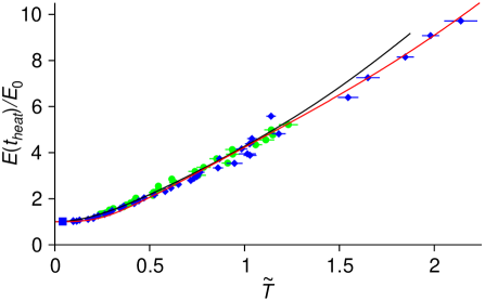
Figure 1: Total energy versus temperature. For each heating time $t_{heat}$, the temperature parameter $\tilde{T}$ is measured from the cloud profile, and the total energy $E(t_{heat})$ is calculated from Eq. (2) in units of the ground state energy $E_{0}$. Green circles: noninteracting Fermi gas data; Blue diamonds: strongly-interacting Fermi gas data. Black curve: predicted energy versus reduced temperature for a noninteracting, trapped Fermi gas, $E_{ideal}(\tilde{T})/E_{ideal}(0)$; Red curve: predicted energy versus $\tilde{T}$ for the unitary case. No temperature calibration is applied since $\tilde{T}\approx\tilde{T}_{nat}$ over the broad temperature range shown. Note that the lowest temperature point (blue square) is constrained to lie on the black curve.

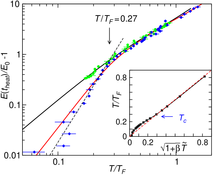
Figure 2: Energy input versus temperature from Fig. 1 after temperature calibration on a $log-log$ scale. The strongly-interacting Fermi gas shows a transition in behavior near $T/T_{F}=0.27$. Green circles: noninteracting Fermi gas data; Blue diamonds: strongly-interacting Fermi gas data; Red (Black) curve: prediction for a unitary (noninteracting), Fermi gas in a Gaussian trap as in experiment; Black dashed line: best fit power law $97.3\,(T/T_{F})^{3.73}$ to the unitary data for $T/T_{F}\leq 0.27$. The inset shows the calibration curve, which has been applied to the unitary data (blue diamonds). The red dashed line in the inset represents the diagonal, $T/T_{F}=\sqrt{1+\beta}\,\tilde{T}$. Here $E_{0}\equiv E(T=0)$.

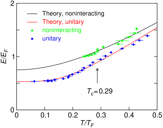
Figure 3: Low temperature comparison of present theory (red, black curves) and experiments (symbols) in terms of $E/E_{F}$ ($E_{F}=k_{B}T_{F}$) per atom as a function of $T/T_{F}$, for both unitary and noninteracting gases in a Gaussian trap. The fact that the two experimental (and the two theoretical) curves do not merge until higher $T^{*}>T_{c}$ is consistent with the presence of a pseudogap.

Supporting Online Material

Computation of Thermodynamical Quantities

The theoretical community is in the midst of unraveling the nature of resonantly interacting fermionic superfluids  (?, ?, ?, ?, ?, ?, ?, ?, ?) with particular emphasis on the strongly interacting Fermi gas  (?). In the BCS-BEC crossover picture  (?), the strongly interacting Fermi gas is intermediate between the weak coupling BCS and BEC limits. In addressing the nature of the excitations from the conventional mean field or BCS-like ground state  (?), our theoretical calculations help to provide a theoretical calibration of the experimental thermometry, and elucidate the thermodynamics.

Without doing any calculations one can anticipate a number of features of thermodynamics in the crossover scenario. The excitations are entirely bosonic in the BEC regime, exclusively fermionic in the BCS regime, and in between both types of excitation are present. In the so-called one-channel problem the “bosons” correspond to noncondensed Cooper pairs, whereas in two-channel models, these Cooper pairs are strongly hybridized with the molecular bosons of the closed channel, singlet state. Below $T_{c}$ the presence of the condensate leads to a single-branch bosonic excitation spectrum which, at intermediate coupling, is predominantly composed of large Cooper pairs. These latter bosons lead to a pseudogap  (S?, ?) above $T_{c}$. Within the conventional mean field ground state, and over the entire crossover regime  (?) below $T_{c}$, the bosons with effective mass $M^{*}$ have dispersion $\Omega_{q}=\hbar^{2}q^{2}/2M^{*}$. This form for the dispersion reflects the absence of direct boson-boson interactions. In the extreme BEC limit, when the fermionic degrees of freedom become irrelevant, direct inter-boson interactions must be accounted for. While our focus in this paper is on the unitary case, when we refer to “BEC” we restrict our attention to the near-unitary BEC regime.

As long as the attractive interactions are stronger than those of the BCS regime, these noncondensed pairs must show up in thermodynamics, as must the pseudogap in the fermionic spectrum. These are two sides of the same coin. Below $T_{c}$, the fermionic excitations have dispersion $E_{\mathbf{k}}=\sqrt{(\epsilon_{\mathbf{k}}-\mu)^{2}+\Delta^{2}}$, where $\epsilon_{\mathbf{k}}=\hbar^{2}k^{2}/2m$ and $\mu$ are the atomic kinetic energy and fermionic chemical potential, respectively. That this excitation gap $\Delta$ is non-zero at $T_{c}$ in the Bogoliubov quasi-particle spectrum $E_{\mathbf{k}}$, differentiates the present approach  (S?) from all other schemes which address BCS-BEC crossover at finite $T$. The bosons, by contrast, are gapless in the superfluid phase, due to their vanishing chemical potential. Within a trap, and in the fermionic regime (for which $\mu>0$), the fermionic component will have a strong spatial inhomogeneity via the spatial variation of the gap. Thus, in contrast to the homogeneous case, fermions on the edge of the trap, which have relatively small or vanishing excitation gaps $\Delta$, will contribute power law dependences to the thermodynamics.

Starting at a magnetic field well above a Feshbach resonance, by decreasing the magnetic field, we tune from the BCS-like regime towards unitarity at resonance. We first consider low $T$ where fermions become paired over much of the trap. The unpaired fermions at the edge tend to dominate the thermodynamics associated with the fermionic degrees of freedom, and lead to a higher (than linear) power law in the $T$ dependence of the entropy. The contribution from excited pairs of fermions is associated with a $T^{3/2}$ dependence of entropy on temperature which dominates for temperatures $T/T_{F}\lesssim 0.05$ or $T/T_{c}\lesssim 0.2$. In general, the overall exponent of the low $T$ power law varies with magnetic field, depending on the magnitude of the gap and temperature, as well as the relative weight of fermionic and bosonic contributions. In the superfluid phase, at all but the lowest temperatures, the fermions and bosons combine to yield $S\propto T^{2}$ precisely at resonance ($(k_{F}a)^{-1}=0$). For the near-unitary case investigated in the paper ($(k_{F}a)^{-1}=0.11$), we have $S\propto T^{1.9}$.

Because our calculations  (?) are based on the standard mean field ground state  (S?), we differ from other work (S?, ?) at finite temperatures. Elsewhere  (S?, S?, ?) we have characterized in quantitative detail the characteristic gap $\Delta$ and pseudogap $\Delta_{pg}$ energy scales. The pseudogap (which is to be associated with a hybridized mix of noncondensed fermion pairs and molecular bosons) and the superfluid condensate (sc) called $\tilde{\Delta}_{sc}$, add in quadrature to determine the fermionic excitation spectrum: $\Delta^{2}(T)=\tilde{\Delta}_{sc}^{2}(T)+\Delta_{pg}^{2}(T)$. Our past work  (S?, S?, S?) has primarily focussed below $T_{c}$. Here we extend these results, albeit approximately, above $T_{c}$. Our formalism has been applied below $T_{c}$ with some success in Ref.  (S?) to measurements of the pairing gap in RF spectroscopy. A more precise, but numerically more complex method for addressing the normal state was given in Ref.  (?).

After including the trap potential $U(r)$ and internal binding energy of the bosons, the local energy density can be decomposed into fermionic ($E_{f}$) and bosonic ($E_{b}$) contributions and directly computed as follows

$$E = \mu n(r)+E_{f}+E_{b}\,,$$

$$E_{f} = \sum_{K}(i\omega_{n}+\epsilon_{\mathbf{k}}-\mu(r))G(K)$$

$$= \sum_{\mathbf{k}}[2E_{\mathbf{k}}f(E_{\mathbf{k}})-(E_{\mathbf{k}}-\epsilon_{\mathbf{k}}+\mu(r))]+\Delta^{2}\chi(0)\,,$$

$$E_{b} = \sum_{q}(\Omega_{\mathbf{q}}-\mu_{boson})\,b(\Omega_{\mathbf{q}}-\mu_{boson})\,,$$ (S1)

where $\mu(r)=\mu-U(r)$, $n(r)$ is the local density, $\omega_{n}=(2n+1)\pi k_{B}T$ is the fermionic Matsubara frequency, $G(K)$ is the renormalized fermionic Green’s function with four-momentum $K\equiv(i\omega_{n},\mathbf{k})$, $b(x)$ and $f(x)$ are the Bose and Fermi distribution functions, respectively. The pair susceptibility $\chi(0)$, at zero frequency and zero momentum, is given by

$$\chi(0)=\sum_{\bf k}\frac{1-2f(E_{\mathbf{k}})}{2E_{\mathbf{k}}}$$ (S2)

and the bosonic chemical potential $\mu_{boson}$ is zero in the superfluid phase.

Unlike the situation in condensed matter systems, for these ultracold gases, thermometry is less straightforward. Experimentally, temperature is determined from the spatial profiles of the cold gas, either in the trap, or following expansion. For weakly interacting Bose and Fermi gases, where the theoretical density is well understood, this procedure is straightforward. However, for a strongly interacting gas, the spatial profile has not been understood until recently  (S?). For this reason, the temperature is often measured on either side far away from the Feshbach resonance, where the scattering length is small. A strongly interacting sample in the unitary regime is then prepared by an adiabatic change of the magnetic field.

More specifically, in the BCS or weak attraction regime, temperature is determined by fitting the spatial (or momentum distribution) profiles to those of a non-interacting Fermi gas  (?). In the opposite BEC regime, temperature can be deduced by fitting the Gaussian wings of density profiles or determining condensate fractions  (?, ?). Thus, it is convenient to describe a given intermediate regime which is accessed adiabatically, by giving the initial temperature at either endpoint. In order to determine this adiabatically accessed temperature, one needs precise knowledge of the entropy $S$ as a function of $T$ and magnetic field from BCS to BEC. The entropy $S$ can be calculated directly  (S?) as a sum of fermionic and bosonic contributions based on the two types of excitations. Equivalently, one can also calculate the entropy from the energy, $S=\int_{0}^{T}\frac{dT}{T}\frac{dE}{dT}$.

In the strongly interacting regime, one can measure an empirical temperature $\tilde{T}$ by fitting a T-F density profile directly to the spatial distribution, as done in this paper. In the following, we describe a temperature calibration method which relates the measured empirical temperature $\tilde{T}$ to the theoretical value of $T/T_{F}$.

Calibration of Experimental Temperature Scale

In order to obtain a temperature calibration curve for the experiments (inset, Fig. 2 main text) we note that our theoretically generated profiles yield very good agreement with the Thomas-Fermi functional form  (S?) for the normal and superfluid states. However, there are slight systematic deviations from this form in the superfluid phase. Below $T_{c}$ the profiles contain the superfluid condensate as well as non-condensed pairs along with excited fermions. Although our profiles are generated for an isotropic trap, it can easily be shown that trap anisotropy is not relevant for thermodynamic quantities. Because they involve integrals over the entire trap, the calculations can be mapped onto an equivalent isotropic system.

Our theoretical profiles are generated for given reduced temperatures $T/T_{F}$. If one applies the experimental procedure to these theoretical profiles one can deduce the parameter $\sqrt{1+\beta}\,\tilde{T}$ for each $T/T_{F}$. Theoretically, then, it is possible to relate these two temperature scales. This is summarized by the calibration curve in the inset to Figure 2.

Quite remarkably, it can be seen from this inset that the experimental T-F fitting procedure yields the precise theoretical temperature in the normal state. This applies even below the pseudogap onset temperature $T^{*}$, since the non-condensed pairs and the fermions both are thermally distributed. However, in the superfluid phase, the parameter $\sqrt{1+\beta}\,\tilde{T}$ systematically underestimates the temperature, because of the presence of a condensate. One can understand this effect as arising principally from the fact that the region of the trap occupied by the condensate is at the center and decreases in radius as temperature is increased, until it vanishes at $T_{c}$. This prevents the profile from expanding with temperature as rapidly as for the non-interacting fermions of strict T-F theory. Hence, one infers an apparently lower temperature. As $T/T_{F}$ approaches zero, the parameter $\sqrt{1+\beta}\,\tilde{T}$ must approach zero as well.

Experimental Methods and Empirical Thermometry

Preparation of the strongly interacting Fermi gas is described in the main text and the details can be found elsewhere  (S?, ?, ?).

Preparation of degenerate, noninteracting Fermi gases follows a similar series of steps. As described previously  (S?), 23 s of forced evaporation at 300 G brings the temperature of the gas to $\tilde{T}=0.24$, the lowest temperature we can achieve in this case. The gas is then heated as described in the main text. Finally, the gas is released and imaged at 526 G to determine the number of atoms and the temperature. Temperatures $\tilde{T}$ between 0.24 and 1.23 are obtained for the noninteracting gas.

All heating and release for time of flight measurements are conducted at 4.6% of the full trap depth. At this depth, the measured trap frequencies, corrected for anharmonicity, are $\omega_{\perp}=\sqrt{\omega_{x}\omega_{y}}=2\pi\times 1696(10)$ Hz and $\omega_{z}=2\pi\times 72(5)$ Hz, so that $\bar{\omega}=(\omega_{x}\omega_{y}\omega_{z})^{1/3}=2\pi\times 592(14)$ Hz is the mean oscillation frequency.

For both the interacting and noninteracting samples, the column density is obtained by absorption imaging of the expanded cloud after 1 ms time of flight, using a two-level state-selective cycling transition  (S?, S?). In the measurements, we take optical saturation into account exactly and arrange to have very small optical pumping out of the two-level system. The resulting absorption image of the cloud can then be analyzed to determine the temperature of the sample.

Anharmonic Corrections to the Energy Input

Eq. 2 of the main text does not include corrections to the energy input which arise from anharmonicity in the gaussian beam trapping potential. In general, after the cloud expands for a time $t_{heat}$, the energy changes when the trapping potential $U(\mathbf{x})$ is abruptly restored,

$$\Delta E(t_{heat})=\int d^{3}\mathbf{x}[n(\mathbf{x},t_{heat})-n_{0}(\mathbf{x})]U(\mathbf{x})\,.$$ (S3)

Here $n(\mathbf{x},t_{heat})$ ($n_{0}(\mathbf{x})$) is the density of the expanded (trapped) cloud, where $n_{0}(\mathbf{x})$ is a zero temperature T-F profile, as noted in the main text. A scale transformation  (S?, ?) relates $n(\mathbf{x},t_{heat})$ to $n_{0}(\mathbf{x})$. Using this result, we obtain Eq. 2 of the main text as well as the anharmonic correction $\Delta E$ arising for a gaussian beam trapping potential. For a cylindrically symmetric trap, we obtain,

$$\frac{\Delta E}{E_{0}}=-\frac{\mu_{0}}{30\,U_{0}}\,\left[\,2b_{\perp}^{4}(t)+b_{\perp}^{2}(t)-3\,\right]+\frac{\mu_{0}^{2}}{360\,U_{0}^{2}}\,\left[\,4b_{\perp}^{6}(t)+2b_{\perp}^{4}(t)+3b_{\perp}^{2}(t)-9\,\right].$$ (S4)

Note that for our experiments, we assume a gaussian beam potential with three different dimensions. These corrections are most significant for the largest values of $t_{heat}$, since the largest contribution to the energy change arises from atoms at the edges of the cloud.

Energy Input for Noninteracting Samples

Although the interacting and noninteracting samples are heated in the same fashion, there are a few differences in the way the energy input is calculated. In the noninteracting case, the correction factor in Eq. 2 of the main text, $\eta_{nonint}$, is determined at the lowest temperature $\tilde{T}=0.24$ from the energy for an ideal Fermi gas. Furthermore, whereas the strongly interacting gas expands hydrodynamically, expansion of the noninteracting gas is ballistic so that $b_{\perp}(t_{heat})=b^{B}_{\perp}(t_{heat})=\sqrt{1+(\omega_{\perp}t_{heat})^{2}}$.

Determination of $\beta$

We determine $\beta$ by comparing the measured Fermi radius for the strongly interacting sample $\sigma_{x}^{\prime}$ to the calculated radius for a noninteracting gas $\sigma_{x}$ confined in the same potential. The relation is given by $\sigma^{\prime}_{x}=\sigma_{x}(1+\beta)^{1/4}$  (?), where $\sigma_{x}=\sqrt{2k_{B}T_{F}/(M\omega_{x}^{2})}$ is the radius for a noninteracting gas. We obtain $\sigma_{x}=1.065\,(N/2)^{1/6}\,\mu$m for our trap parameters. This calculated radius is consistent with the value measured for noninteracting samples at 526 G in our trap. To determine $\sigma_{x}^{\prime}$, we measure the size of the cloud after 1 ms of expansion, and scale it down by the known hydrodynamic expansion factor of $b^{H}_{\perp}(1\,\mbox{ms})=13.3$  (S?, S?). We then determine the Fermi radius $\sigma_{x}^{\prime}=11.98\,(N/2)^{1/6}\,\mu\mbox{m}/13.3=0.901(0.021)\,(N/2)^{1/6}\mu$m. With these results, we obtain $\beta=-0.49(0.04)$ (statistical error only).

Observed Transition in Energy versus Empirical Temperature $\tilde{T}$

For the strongly interacting Fermi gas, without calibrating the empirical temperature scale, we observe a transition between two patterns of behavior at $\tilde{T}=0.33$  (?): For $\tilde{T}=0.33-2.15$, we find that the energy closely corresponds to that of a trapped Fermi gas of noninteracting atoms with the mass scaled by $1/(1+\beta)$. At temperatures between $\tilde{T}=0.04-0.33$, the energy scales as $\tilde{T}^{2.53}$, significantly deviating from ideal gas behavior as can be seen in Fig. S1. The transition between two power laws is evident in the slope change of the $log-log$ plot of Fig. S2.

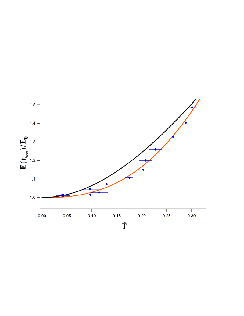
Figure S1: Strongly-interacting Fermi gas below the transition temperature. $E/E_{0}$ versus uncalibrated empirical temperature $\tilde{T}$ on a linear scale. Orange line, best fit power law $9.8\,\tilde{T}^{2.53}$. Black curve: Predicted $E/E_{0}$ for an ideal Fermi gas as a function of $\tilde{T}=T/T_{F}$. Note the lowest temperature point (blue square) is not included in the fits: It is constrained to lie on the black curve by our choice of $\eta_{int}=1.01$ in Eq. 2 of the main text.

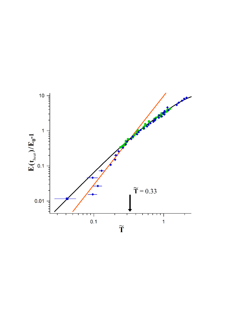
Figure S2: Energy input versus uncalibrated temperature $\tilde{T}$ on a $log-log$ scale. The strongly interacting Fermi gas shows a transition in behavior near $\tilde{T}=0.33$. Green circles: noninteracting Fermi gas data; Blue diamonds: strongly interacting Fermi gas data. Black curve, prediction for a noninteracting, trapped Fermi gas. Orange line, best fit power law $9.8\,\tilde{T}^{2.53}$. Note the lowest temperature point (blue square) is not included in the fits, as it is constrained to lie on the black curve.

References and Notes

- 1. K. M. O’Hara, S. L. Hemmer, M. E. Gehm, S. R. Granade, J. E. Thomas, Science 298, 2179 (2002).
- 2. J. E. Thomas, M. E. Gehm, Am. Scientist 92, 238 (2004).
- 3. H. Heiselberg, Phys. Rev. A 63, 043606 (2001).
- 4. T.-L. Ho, Phys. Rev. Lett. 92, 090402 (2004).
- 5. J. G. A. Baker, Phys. Rev. C 60, 054311 (1999).
- 6. J. Carlson, S.-Y. Chang, V. R. Pandharipande, K. E. Schmidt, Phys. Rev. Lett. 91, 050401 (2003).
- 7. A. Perali, P. Pieri, G. C. Strinati, Phys. Rev. Lett. 93, 100404 (2004).
- 8. M. E. Gehm, S. L. Hemmer, S. R. Granade, K. M. O’Hara, J. E. Thomas, Phys. Rev. A 68, 011401(R) (2003).
- 9. T. Bourdel, et al., Phys. Rev. Lett. 93, 050401 (2004).
- 10. M. Bartenstein, et al., Phys. Rev. Lett. 92, 120401 (2004).
- 11. M. Houbiers, et al., Phys. Rev. A 56, 4864 (1997).
- 12. R. Combescot, Phys. Rev. Lett. 83, 3766 (1999).
- 13. M. Holland, S. J. J. M. F. Kokkelmans, M. L. Chiofalo, R. Walser, Phys. Rev. Lett. 87, 120406 (2001).
- 14. E. Timmermans, K. Furuya, P. W. Milonni, A. K. Kerman, Phys. Lett. A 285, 228 (2001).
- 15. Y. Ohashi, A. Griffin, Phys. Rev. Lett. 89, 130402 (2002).
- 16. J. Stajic, et al., Phys. Rev. A 69, 063610 (2004).
- 17. Q. Chen, J. Stajic, S. Tan, K. Levin (2004). ArXiv:cond-mat/0404274.
- 18. C. A. Regal, M. Greiner, D. S. Jin, Phys. Rev. Lett. 92, 040403 (2004).
- 19. M. W. Zwierlein, et al., Phys. Rev. Lett. 92, 120403 (2004).
- 20. C. Chin, et al., Science 305, 1128 (2004).
- 21. J. Kinast, S. L. Hemmer, M. E. Gehm, A. Turlapov, J. E. Thomas, Phys. Rev. Lett. 92, 150402 (2004).
- 22. M. Bartenstein, et al., Phys. Rev. Lett. 92, 203201 (2004).
- 23. J. Kinast, A. Turlapov, J. E. Thomas, Phys. Rev. A 70, 051401(R) (2004).
- 24. F. London, Phys. Rev. 54, 947 (1938).
- 25. J. Kinast, A. Turlapov, J. E. Thomas (2004). ArXiv:cond-mat/0409283.
- 26. Materials and methods are available as supporting material on Science Online.
- 27. Q. Chen, J. Stajic, K. Levin (2004). ArXiv:cond-mat/0411090.
- 28. Q. J. Chen, K. Levin, I. Kosztin, Phys. Rev. B 63, 184519 (2001).
- 29. A. J. Leggett, Modern Trends in the Theory of Condensed Matter (Springer-Verlag, Berlin, 1980), pp. 13–27.
- 30. J. Kinnunen, M. Rodríguez, P. Törmä, Science 305, 1131 (2004).
- 31. L. D. Carr, G. V. Shlyapnikov, Y. Castin, Phys. Rev. Lett. 92, 150404 (2004).
- 32. J. E. Williams, N. Nygaard, C. W. Clark, New J. Phys. 6, 123 (2004).
- 33. S. Stringari, Europhys. Lett. 65, 749 (2004).
- 34. H. Hu, A. Minguzzi, X.-J. Liu, M. P. Tosi, Phys. Rev. Lett. 93, 190403 (2004).
- 35. H. Heiselberg, Phys. Rev. Lett. 93, 040402 (2004).
- 36. J. Stajic, Q. Chen, K. Levin (2004). ArXiv:cond-mat/0408104.
- 37. C. Menotti, P. Pedri, S. Stringari, Phys. Rev. Lett. 89, 250402 (2002).
- 38. B. Jackson, P. Pedri, S. Stringari, Europhys. Lett. 67, 524 (2004). Our fit method is derived from ideas presented in this paper.
- 39. M. Bartenstein, et al. (2004). ArXiv:cond-mat/0408673.
-
1.

References and Notes

- S1. T.-L. Ho, Phys. Rev. Lett. 92, 090402 (2004).
- S2. A. Perali, P. Pieri, L. Pisani, G. C. Strinati, Phys. Rev. Lett. 92, 220404 (2004).
- S3. L. D. Carr, G. V. Shlyapnikov, Y. Castin, Phys. Rev. Lett. 92, 150404 (2004).
- S4. J. E. Williams, N. Nygaard, C. W. Clark, New J. Phys. 6, 123 (2004).
- S5. H. Heiselberg, Phys. Rev. Lett. 93, 040402 (2004).
- S6. H. Hu, A. Minguzzi, X.-J. Liu, M. P. Tosi, Phys. Rev. Lett. 93, 190403 (2004).
- S7. S. Stringari, Europhys. Lett. 65, 749 (2004).
- S8. J. Kinnunen, M. Rodriguez, P. Törmä, Science 305, 1131 (2004).
- S9. C. Chin (2004). ArXiv:cond-mat/0409489.
- S10. K. M. O’Hara, S. L. Hemmer, M. E. Gehm, S. R. Granade, J. E. Thomas, Science 298, 2179 (2002).
- S11. Q. Chen, J. Stajic, S. Tan, K. Levin (2004). ArXiv:cond-mat/0404274.
- S12. A. J. Leggett, Modern Trends in the Theory of Condensed Matter (Springer-Verlag, Berlin, 1980), pp. 13–27.
- S13. J. Stajic, Q. J. Chen, K. Levin (2004). ArXiv:cond-mat/0402383.
- S14. J. Stajic, et al., Phys. Rev. A 69, 063610 (2004).
- S15. Q. Chen, J. Stajic, K. Levin (2004). ArXiv:cond-mat/0411090.
- S16. A. Perali, P. Pieri, G. C. Strinati, Phys. Rev. Lett. 93, 100404 (2004).
- S17. J. Stajic, Q. Chen, K. Levin (2004). ArXiv:cond-mat/0408104.
- S18. J. Maly, B. Jankó, K. Levin, Physica C 321, 113 (1999).
- S19. C. A. Regal, M. Greiner, D. S. Jin, Phys. Rev. Lett. 92, 040403 (2004).
- S20. M. Bartenstein, et al., Phys. Rev. Lett. 92, 120401 (2004).
- S21. M. W. Zwierlein, et al., Phys. Rev. Lett. 92, 120403 (2004).
- S22. J. Kinast, et al., Phys. Rev. Lett. 92, 150402 (2004).
- S23. J. Kinast, A. Turlapov, J. E. Thomas, Phys. Rev. A 70, 051401(R) (2004).
- S24. C. Menotti, P. Pedri, S. Stringari, Phys. Rev. Lett. 89, 250402 (2002).
- S25. M. E. Gehm, S. L. Hemmer, S. R. Granade, K. M. O’Hara, J. E. Thomas, Phys. Rev. A 68, 011401(R) (2003).
- S26. J. Kinast, A. Turlapov, J. E. Thomas (2004). ArXiv:cond-mat/0409283.