SU(4) Model of High-Temperature Superconductivity:
Manifestation of Dynamical Symmetry in Cuprates

Abstract

The mechanism that leads to high-temperature superconductivity in cuprates remains an open question despite intense study for nearly two decades. Here, we introduce an SU(4) model for cuprate systems having many similarities to dynamical symmetries known to play an important role in nuclear structure physics and in elementary particle physics. Analytical solutions in three dynamical symmetry limits of this model are found: an SO(4) limit associated with antiferromagnetic order; an SU(2) limit that may be interpreted as a $d$-wave pairing condensate; and an SO(5) limit that may be interpreted as a doorway state between the antiferromagnetic order and the superconducting order. It is demonstrated that with a slightly broken SO(5) but under constraint of the parent SU(4) symmetry, the model is capable of describing the rich physics that is crucial in explaining why cuprate systems that are antiferromagnetic Mott insulators at half filling become superconductors through hole doping.

I Introduction

Describing collective motion in a strongly correlated many-body system in terms of single particle degrees of freedom is sometimes not feasible. Even if one can solve the problem with the help of large-scale numerical calculations, such a practice may not always be interesting because physics can be totally buried in the numerous configurations used in the calculation. In the cuprate systems exhibiting high-temperature superconducting (SC) properties, there is a substantial point of view (see, for example, Ref. An00 ) that the many-body correlations are so strong that the dynamics can no longer be described meaningfully in terms of individual particles. On the other hand, similar questions were also asked long ago in nuclear physics. Nuclear physicists have developed a completely different approach to solve the many-body problems. The approach is based on the fact that collective motions in such quantum many-body systems are often governed by only a few collective degrees of freedom. Once these degrees of freedom are identified and properly incorporated into a model, calculations may become feasible and, most importantly, the physics may become transparent. One systematic way of identifying the relevant collective degrees of freedom in a many-body system is the method of dynamical symmetries.

A quantum system exhibiting dynamical symmetries usually contains two or more competing collective modes. In nuclear physics, it has long been known that the transition from spherical nuclei, which dominate the beginnings and endings of nucleonic shells, to deformed nuclei, which often dominate the middle of shells, is controlled by the microscopic competition between long-range quadrupole-quadrupole interactions favoring deformed rotational mode and short-range monopole pairing interactions favoring spherical vibrational mode. This competition in nuclear physics may be expressed algebraically as a competition between a dynamical symmetry that favors pairing and a dynamical symmetry that favors multipole (particle–hole) interactions FDSM ; IBM . Besides nuclear physics, the dynamical symmetry method has also been applied in molecular physics Mole1 ; Mole2 and particle physics Part .

In cuprates, it is now widely agreed that the mechanism responsible for superconductivity is closely related to the unusual antiferromagnetic (AF) insulator properties of their normal states. There are also compelling arguments that the pair mechanism leading to high-temperature superconductivity does not correspond to ordinary BCS $s$-wave pairing. Although experimental evidence implicates singlet (hole) pairs as the carriers of the supercurrent, the interaction leading to the formation of the singlet pairs appears not to be the traditional lattice phonon mechanism underlying the BCS theory, but rather seems to originate in strong electron correlations. Furthermore, the pairing gap is anisotropic, with nodes in the $k_{x}$–$k_{y}$ plane strongly suggestive of $d$-wave hybridization in the 2-particle wavefunctions.

Such observations argue strongly for a theory based on continuous symmetries of the dynamical system that is capable of describing more sophisticated pairing than found in the simple BCS picture (which is described by a single complex order parameter), and capable of unifying SC and AF collective modes and the corresponding phases on an equivalent footing. Then such fundamentally different physics as SC order and AF order can emerge from the same effective Hamiltonian as concentration variables (e.g., doping parameters) are varied. In this manuscript, we report on an SU(4) model that we have recently developed su4a ; su4b ; su4c ; su4d aiming at understanding the mechanism that leads to high-temperature superconductivity in cuprates. Theoretical models employing algebras and groups can be found in the field of condensed matter (for recent examples, see Refs. Zh97 ; Others ). However, to our knowledge, the powerful dynamical symmetry method of the type that we shall describe below has not been applied systematically in this field.

II Dynamical Symmetry Method

A system possesses dynamical symmetries if the Hamiltonian can be expressed as a polynomial in the Casimir invariants of a subgroup chain. For approximately the same period of time that the high-Tc compounds have been known, techniques based on dynamical symmetries in fermion degrees of freedom have been in development in the field of nuclear structure physics FDSM . There it has proven fruitful to ask the following questions: what are the most important collective degrees of freedom in the low-lying spectrum of complex nuclei, what are the microscopic many-body quantum operators that create and annihilate these modes, and what is the commutator algebra obeyed by this set of operators?

Systematic investigation of these questions has led to strong confirmation of the following set of conjectures about the nuclear many-body system: (1) Low-lying collective modes are in approximate one-to-one correspondence with dynamical symmetries in the fermion degrees of freedom. (2) A dynamical symmetry corresponding to low-lying collective modes is associated with a Lie algebra and its subalgebras that are formed from a set of fermion operators closed under commutation. (3) Different dynamical symmetry subgroup chains arising from the same highest symmetry group are associated with fundamentally different phases of the theory. These phases are unified in the highest group. (4) The unification implied by the preceding point suggests that the many low-lying collective states formed by systematic filling of valence shells in heavy nuclei are in reality different projections in an abstract multidimensional space of the same state. Equivalently, the different states are transformed into each other by the generators of the symmetry. Thus, the systematics of collective modes and phase transitions as a function of concentration variables are specified by the group structure.

Motivated by the observation that in a nuclear system at low-energy excitation, valence nucleon pairs tend to correlate strongly to form $s$ (spin 0) pairs and $d$ (spin 2) pairs, Wu, Feng, and Guidry introduced $s$ and $d$ fermion pairs as the basic building blocks of the Fermion Dynamical Symmetry Model FDSM . These pair operators, when supplemented with the multipole operators, close either an $SO(8)$ or an $Sp(6)$ algebra, depending on the choice of the basis FDSM . If one neglects the fermionic degrees of freedom of these pairs and treats them as bosons, one has the early Interacting Boson Model IBM of Arima and Iachello. All the dynamical symmetries emerging from these models have found correspondence with the known low-lying collective modes in nuclear systems, such as the spherical vibrational mode, deformed rotational mode, and $\gamma$-unstable collective mode.

It has been demonstrated that dynamical symmetries of the type described in Ref. FDSM are realized to remarkably high accuracy in the spectrum and the wavefunctions of microscopic calculations using the Projected Shell Model sun98 ; sun02 . Since this model is of the shell-model type based on single-particle degrees of freedom, and is known to give extremely good agreement with a broad range of experimental data (see, e.g., Ref. sun97 ), this provides rather conclusive proof that these dynamical symmetries are strongly realized in the low-lying states of complex nuclei. This raises the issue of whether similar symmetries might be found in other complex many-body fermion systems such as those important in condensed matter.

The dynamical symmetry method applied in cuprates corresponds schematically to the following algorithm:

0. Assume the following conjecture: All strongly collective modes in fermion (or boson) many-body systems can be put into correspondence with a closed algebra defining a dynamical symmetry of the sort described below. This is a conjecture, but there is so much evidence in support of it from various fields of physics that it is almost a theorem: Strongly correlated motion implies a symmetry of the dynamics described by a Lie algebra in the second-quantized operators implementing that motion.

1. Identify, within a suitable “valence space”, degrees of freedom that one believes are physically relevant for the problem at hand, guided by phenomenology, theory, and general principles. In the present case, that reduces to defining a minimal set of operators that might be important to describe superconductivity and antiferromagnetism.

2. Try to close a commutation algebra (of manageable dimension) with the second-quantized operators creating and annihilating the modes chosen in step 1. If necessary, approximate these operators, or add additional ones to the set if the algebra does not close naturally.

3. Use standard Lie algebra theory to identify relevant subalgebra chains that end in algebras for conservation laws that one expects to be obeyed for the problem at hand. In the present example, we require all group chains to end in $U(1)\times SU(2)$, corresponding to an algebra implementing conservation of charge and spin.

4. Construct dynamical symmetry Hamiltonians (Hamiltonian that are polynomials in the Casimir invariants of a group chain) for each chain. Each such group chain thus defines a wavefunction basis labeled by the eigenvalues of chain invariants (the Casimirs and the elements of the Cartan subalgebras), and a Hamiltonian that is diagonal in that basis (since it is constructed explicitly from invariants). Thus, the Schoedinger equation is solved analytically for each chain, by construction.

5. Calculate the physical implications of each of these dynamical symmetries by considering the wavefunctions, spectra, and transitional matrix elements of physical relevance. This is tractable, because the eigenvalues and eigenvectors were obtained in step 4. Consistency of the symmetry requires that transition operators be related to group generators; otherwise transitions would mix irreducible multiplets and break the symmetry.

6. If step 5 suggests that one is on the right track (meaning that a wise choice was made in step 1), one can write the most general Hamiltonian for the system in the model space, which is just a linear combination of all the Hamiltonians for the symmetry group chains. Since the Casimir operators of different group chains do not generally commute with each other, a Casimir invariant for one group chain may be a symmetry-breaking term for another group chain. Thus the competition between different dynamical symmetries and the corresponding phase transitions can be studied.

7. The symmetry-limit solutions may be used as a starting point for more ambitious calculations that incorporate symmetry breaking. Although no longer generally analytical, such more realistic approximations may be solved by perturbation theory around the symmetry solutions (which are generally non-perturbative, so this is perturbation theory around a non-perturbative minimum), by numerical diagonalization of symmetry breaking terms, or by coherent state method as shown later.

Of course, in practical calculations only a few carefully selected degrees of freedom can be included and the effect of the excluded space must be incorporated by renormalized interactions in the truncated space. It follows that the validity of such an approach hinges on a wise choice of the collective degrees of freedom and sufficient phenomenological or theoretical information to specify the corresponding effective interactions of the truncated space.

III The SU(4) Model

We now introduce a mathematical formalism that provides a systematic implementation of the dynamical symmetry procedure for cuprate systems.

III.1 Choice of operators and the algebra

The basic assumption of the SU(4) model is that the configuration space relevant for competing superconductivity and antiferromagnetism is built from coherent pairs formed from two electrons (or holes) centered on adjacent lattice sites. In cuprates the coherent pairs are believed to exhibit $d$-wave orbital symmetry Sc95 , suggesting coexistence of two kinds of coherent pairs in a minimal model: the spin-singlet ($p$) and the spin-triplet ($q$) pairs. We adopt the $d$-wave pairs with structure defined in Refs. De95 ; Zh97 as the basic dynamical building blocks of the SU(4) model

$$\begin{array}[]{ll}\displaystyle p_{12}^{\dagger}=\sum_{k}g(k)c_{k\uparrow}^{\dagger}c_{-k\downarrow}^{\dagger}&p_{12}=(p^{\dagger}_{12})^{\dagger},\\ \displaystyle q_{ij}^{\dagger}=\sum_{k}g(k)c_{k+Q,i}^{\dagger}c_{-k,j}^{\dagger}&q_{ij}=(q^{\dagger}_{ij})^{\dagger},\end{array}$$ (1)

where $c_{k,i}^{\dagger}$ creates an electron of momentum $k$ and spin projection $i,j=1{\rm\ or\ }2\ (\equiv\uparrow$ or $\downarrow)$, $g(k)=(\cos k_{x}-\sin k_{y})$ is the $d$-wave form factor, and $Q=(\pi,\pi,\pi)$ is an AF ordering vector. These pair operators, when supplemented with operators of particle-hole type ${Q}_{ij}$ and $S_{ij}$,

$${Q}_{ij}=\sum_{k}c_{k+Q,i}^{\dagger}c_{k,j}\qquad S_{ij}=\sum_{k}c_{k,i}^{\dagger}c_{k,j}-\mbox{$\small\frac{1}{2}$}\Omega\delta_{ij},$$ (2)

constitute a 16-element operator set that is closed su4a under a U(4) $\supset$ U(1) $\times$ SU(4) algebra if the condition

$$g(k)\approx\mbox{sgn}\,(\cos k_{x}-\cos k_{y})$$

is imposed. In Eq. (2), $\Omega$ is the maximum number of doped electrons that can form coherent pairs, assuming the normal state (at half filling) to be the vacuum. The U(1) factor, ${Q}_{+}={Q}_{11}+{Q}_{22}=\sum_{k}(c_{k+Q\uparrow}^{\dagger}c_{k\uparrow}+c_{k+Q\downarrow}^{\dagger}c_{k\downarrow})$, in U(1) $\times$ SU(4) is associated with charge-density waves, which is independent of the SU(4) algebra. For no broken pairs the charge-density waves are excluded in the symmetry limit and in the following discussion we shall restrict attention to the SU(4) group.

The SU(4) group has three dynamical symmetry group chains su4a :

$$\supset {\rm SO(4)}\times{\rm U(1)}\supset{\rm SU(2)_{s}}\times{\rm U(1)}$$

$${\rm SU(4)} \supset {\rm SO(5)}\supset{\rm SU(2)_{s}}\times{\rm U(1)}$$

$$\supset {\rm SU(2)_{p}}\times{\rm SU(2)_{s}}\supset{\rm SU(2)_{s}}\times{\rm U(1)}$$

each of which ends in the subgroup ${\rm SU(2)_{s}}\times{\rm U(1)}$ representing total spin and charge conservation.

The 15 SU(4) generators are related to more physical operators through the linear combinations:

$$\begin{array}[]{rcll}D^{\dagger}&=&p^{\dagger}_{12}\qquad D=p_{12}&d-\mbox{wave singlet pairing (2 operators)}\\ \vec{\pi}^{\dagger}&=&\left(\ i\frac{q_{11}^{\dagger}\ -q_{22}^{\dagger}}{2},\ \frac{q_{11}^{\dagger}+q_{22}^{\dagger}}{2},\ -i\frac{q_{12}^{\dagger}+q_{21}^{\dagger}}{2}\right)\quad\vec{\pi}=(\vec{\pi}^{\dagger})^{\dagger}&d-\mbox{wave triplet pairing (6 operators)}\\ \vec{\cal Q}&=&\left(\frac{{Q}_{12}+{Q}_{21}}{2},-i\frac{{Q}_{12}-{Q}_{21}}{2},\frac{{Q}_{11}-{Q}_{22}}{2}\right)&\mbox{staggered magnetization (3 operators)}\\ \vec{S}&=&\left(\frac{S_{12}+S_{21}}{2},\ -i\,\frac{S_{12}-S_{21}}{2},\ \frac{S_{11}-S_{22}}{2}\right)&\mbox{spin (3 operators)}\\ \hat{n}&=&\sum_{k,i}c_{k,i}^{\dagger}c_{k,i}=S_{11}+S_{22}+\Omega&\mbox{particle number (1 operator)}\end{array}$$ (4)

It will also sometimes prove useful to replace the number operator $\hat{n}$ with the charge operator $M$, defined through $M=\frac{1}{2}(S_{11}+S_{22})=\mbox{$\small\frac{1}{2}$}(\hat{n}-\Omega)$.

III.2 The collective subspace

The group SU(4) has a quadratic Casimir operator

$$C_{su(4)}=D^{\dagger}D+\vec{\pi}^{\dagger}\cdot\vec{\pi}+\vec{\cal Q}\cdot\vec{\cal Q}+\vec{S}\cdot\vec{S}+M(M-4).$$ (5)

The group is rank-3 and the irreducible representations (irreps) may be labeled by 3 weight-space quantum numbers, $(\sigma_{1},\sigma_{2},\sigma_{3})$. We assume for the simplest implementation of the model a collective $d$-wave pair subspace spanned by the following vectors:

$$|S\rangle=|n_{x}n_{y}n_{z}n_{s}\rangle=(\pi_{x}^{\dagger})^{n_{x}}(\pi_{y}^{\dagger})^{n_{y}}(\pi_{z}^{\dagger})^{n_{z}}(D^{\dagger})^{n_{s}}|0\rangle.$$ (6)

This collective subspace is associated with irreps of the form

$$(\sigma_{1},\sigma_{2},\sigma_{3})=(\mbox{$\small\frac{\Omega}{2}$},0,0),$$

where 2$\Omega$ is the dimension of the single-particle space in the SU(4) model, and thus $\Omega$ is the maximum number of pairs that can be accommodated in the model space. The corresponding expectation value of the SU(4) Casimir evaluated in these irreps is a constant,

$$\langle C_{su(4)}\rangle=\mbox{$\small\frac{\Omega}{2}$}(\mbox{$\small\frac{\Omega}{2}$}+4).$$

The dimensionality of the full space is $2^{2\Omega}$. However, the dimensionality of our collective subspace is much smaller, scaling approximately as $\Omega^{4}$:

$${\rm Dim\thinspace}(\mbox{$\small\frac{\Omega}{2}$},0,0)=\mbox{$\small\frac{1}{12}$}(\mbox{$\small\frac{\Omega}{2}$}+1)(\mbox{$\small\frac{\Omega}{2}$}+2)^{2}(\mbox{$\small\frac{\Omega}{2}$}+3).$$

Thus for small lattices it is possible to enumerate all states of the collective subspace in a simple model where observables can be calculated analytically.

III.3 SU(4) model Hamiltonian

The most general 2-body Hamiltonian within the $d$-wave pair space consists of a linear combination of (quadratic) Casimir operators $C_{g}$ for all subgroups $g$

$$H=H_{0}+\sum_{g}H_{g}C_{g},$$

where $H_{g}$ are parameters and the Casimir operators $C_{g}$ are

$$C_{SO(5)} = \vec{\pi}^{\dagger}\cdot\vec{\pi}+\vec{S}\cdot\vec{S}+M(M-3)$$

$$C_{SO(4)} = \vec{\cal Q}\cdot\vec{\cal Q}+\vec{S}\cdot\vec{S}$$

$$C_{SU(2)_{p}} = D^{\dagger}D+M(M-1)$$ (7)

$$C_{SU(2)_{s}} = \vec{S}\cdot\vec{S}$$

$$C_{U(1)} = M\mbox{ and }M^{2}.$$

For fixed electron number the terms in $M$ and $M^{2}$ in Eq. (7) are constant. The term $H_{0}$ is a quadratic function of particle number and may be parameterized as

$$H_{0}=\varepsilon n+\mbox{$\small\frac{1}{2}$}\mbox{v}n(n-1),$$

where $\varepsilon$ and v are the effective single-electron energy and the average two-body interaction in zero-order approximation, respectively. Thus the Hamiltonian can be written as

$$H=H_{0}+V,\qquad V=-G_{0}D^{\dagger}D-G_{1}\vec{\pi}^{\dagger}\cdot\vec{\pi}-\chi\vec{\cal Q}\cdot\vec{\cal Q}+\kappa\vec{S}\cdot\vec{S}$$ (8)

where $G_{0}$, $G_{1}$, $\chi$ and $\kappa$ are the interaction strengths of $d$-wave singlet pairing, $d$-wave triplet pairing, staggered magnetization, and spin–spin interactions, respectively. Since $\langle C_{su(4)}\rangle$ is a constant, by using Eq. (5) we can eliminate the $\vec{\pi}^{\dagger}\cdot\vec{\pi}$ term and after renormalizing the interaction strengths the SU(4) Hamiltonian can be expressed as

$$H=H^{\prime}_{0}-G[\ (1-p)D^{\dagger}D+p\vec{\cal Q}\cdot\vec{\cal Q}\ ]+\kappa_{\rm eff}\,\vec{S}\cdot\vec{S},\qquad H^{\prime}_{0}=\varepsilon_{\rm eff}\,n+\mbox{$\small\frac{1}{2}$}\mbox{v}_{\rm eff}\,n(n-1)$$ (9)

with $(1-p)G=G^{0}_{\rm eff}$, $pG=\chi_{\rm eff}$, and $\kappa_{\rm eff}$ as the effective interaction strengths, and where $0\leq p\leq 1$ for the parameter $p$. Since in this paper we primarily address the ground state properties where $S=0$, the last term in Eq. (9) will generally not enter into the later discussion.

III.4 Physical interpretation for the dynamical symmetries

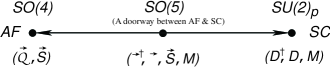
Figure 1: Dynamical symmetries associated with the $U(4)$ symmetry. The generators are listed for each subgroup.

The three subgroup chains of the SU(4) symmetry define three dynamical symmetries with clear physical meanings. The symmetry limits SU(2), SO(4), and SO(5), correspond to the choices $p=0$, 1, and 1/2, respectively, in Eq. (9). The Hamiltonian, eigenfunctions, energy spectrum and the corresponding quantum numbers of these symmetry limits can be explicitly given (see Ref. su4a ). As we shall now discuss, each symmetry limit represents a different possible low-energy phase of the SU(4) system. Fig. 1 illustrates these dynamical symmetries and the relation to the corresponding phases.

The pairing gap $\Delta$ (measure of pairing order) and the staggered magnetization (measure of AF order) $Q$,

$$\Delta=G^{0}_{\rm eff}\langle D^{\dagger}D\rangle^{1/2},\qquad Q=\langle\vec{\cal Q}\cdot\vec{\cal Q}\rangle^{1/2},$$ (10)

may be used to characterize the states in these symmetry limits. We introduce also a relative doping fraction $x$ that is related to particle number and lattice degeneracy through

$$x=1-\frac{n}{\Omega}.$$ (11)

Since $\Omega-n$ is the hole number when $\Omega<n$, positive $x$ represents the case of hole-doping, with $x=0$ corresponding to half filling (no doping) and $x=1$ to maximal doping.

III.4.1 The SO(4) limit

The dynamical symmetry chain

$$SU(4)\supset SO(4)\times U(1)\supset SU(2)_{s}\times U(1),$$

which we shall term the SO(4) limit, corresponds to long-range AF order. This is the symmetry limit of Eq. (9) when $p=1$. The SO(4) subgroup is locally isomorphic to $SU(2)_{F}\times SU(2)_{G}$, where the product group is generated by the linear combinations

$$\vec{F}=\mbox{$\small\frac{1}{2}$}(\vec{\cal Q}+\vec{S}),\qquad\vec{G}=\mbox{$\small\frac{1}{2}$}(\vec{\cal Q}-\vec{S})$$

of the original SO(4) generators $\vec{\cal Q}$ and $\vec{S}$. We may interpret the new generators $\vec{F}$ and $\vec{G}$ physically by noting that if we transform ${\cal Q}_{ij}$ and $S_{ij}$ defined in Eq. (2) to the coordinate lattice space,

$${\cal Q}_{ij} = \sum_{r}(-)^{r}c^{{\dagger}}_{ri}c_{rj}=\sum_{r={\rm even}}c^{{\dagger}}_{ri}c_{rj}-\sum_{r={\rm odd}}c^{{\dagger}}_{ri}c_{rj}$$

$$S_{ij} = \sum_{r}c^{{\dagger}}_{ri}c_{rj}=\sum_{r={\rm even}}c^{{\dagger}}_{ri}c_{rj}+\sum_{r={\rm odd}}c^{{\dagger}}_{ri}c_{rj}$$

implying that $\vec{F}$ is the generator of total spin on even sites and $\vec{G}$ is the generator of total spin on odd sites. Thus, we may interpret the SO(4) group as being generated by two independent spin operators: one that is the total spin on all sites and one that is the difference in spins on even and odd sites of the spatial lattice. This clearly is an algebraic version of the physical picture associated with AF long-range order.

Furthermore, the ground state has maximal staggered magnetization

$$Q=\mbox{$\small\frac{1}{2}$}\Omega(1-x)=\mbox{$\small\frac{1}{2}$}n$$

and a large energy gap (associated with the correlation $\vec{\cal Q}\cdot\vec{\cal Q}$)

$$\Delta E=2\chi_{\rm eff}(1-x)\Omega$$

that inhibits electronic excitation and favors magnetic insulator properties at half filling. In addition, the pairing gap

$$\Delta=\mbox{$\small\frac{1}{2}$}G^{0}_{\rm eff}\Omega\sqrt{x(1-x)}$$

is small near half filling ($x=0$). We thus conclude that these SO(4) states are identified naturally with an AF insulating phase of the system.

III.4.2 The SU(2) limit

The dynamical symmetry chain

$$SU(4)\supset SU(2)_{p}\times SU(2)_{s}\supset SU(2)_{s}\times U(1),$$

which we shall term the SU(2) limit, corresponds to SC order and is the $p=0$ symmetry limit of Eq. (9). In the ground state, there exists a large pairing gap

$$\Delta E=G^{(0)}_{\rm eff}\Omega,$$

the pairing correlation is the largest among the three symmetry limits, and the staggered magnetization vanishes in the ground state:

$$\Delta=\mbox{$\small\frac{1}{2}$}G^{0}_{\rm eff}\Omega\sqrt{1-x^{2}}\ ,\qquad Q=0.$$

Thus we propose that this state is a pair condensate associated with a $d$-wave SC phase of the cuprates.

III.4.3 The SO(5) limit

The dynamical symmetry chain

$$SU(4)\supset SO(5)\supset SU(2)_{s}\times U(1),$$

which we shall term the SO(5) limit, appears when $p=1/2$ in Eq. (9). The SO(5) dynamical symmetry has very unusual behavior. Although the expectation values of $\Delta$ and $Q$ for ground state in this symmetry limit are the same as that of Eq. (III.4.2) for the SU(2) case, there exists a huge number of states with different number of $\pi$ pairs that can mix easily with the ground state when $x$ is small. In particular, at half filling ($x=0$) the ground state is highly degenerate with respect to configurations of different number of $\pi$ pairs. The $\pi$ pairs must be responsible for the antiferromagnetism in this phase, since within the model space only $\pi$ pairs carry spin. Thus the ground state in this symmetry limit has large-amplitude fluctuation in the AF order (and SC order). This indicates that the SO(5) symmetry limit is associated with phases in which the system is extremely susceptible to fluctuations between AF and SC order.

S. C. Zhang proposed to unify AF and SC states by assembling his order parameters into a five-dimensional vector and constructing an SO(5) group that rotates AF order into $d$-wave SC order Zh97 . The Zhang SO(5) group is a subgroup of our SU(4) group, implying that the two models are related to each other. The essential difference is that we implement the full quantum dynamics (commutator algebra) of these operators exactly, while in Ref. Zh97 , the dynamics is implemented in an approximate manner: a subset of ten of the operators acts as a rotation on the remaining five operators $\{D^{\dagger},D,\vec{Q}\}$, which are treated phenomenologically as five independent components of an order-parameter vector (superspin $\vec{n}$). Thus only 10 of the 15 generators of our SU(4) are treated dynamically in the Zhang SO(5) model. If the full quantum dynamics (full commutator algebra) of the 15 operators is taken into account, the symmetry for cuprates must be SU(4), not SO(5).

III.5 Closure of SU(4) and no-double-occupancy constraint

Suppression of double occupancy on sites in the copper oxide planes is critical An87 in explaining why cuprate systems are antiferromagnetic Mott insulators at half filling and become superconductors through hole doping. To realize Mott insulator phases at half-filling it is normal to impose a no-double-occupancy rule – the constraint that each lattice site cannot have more than one valence electron – by Gutzwiller projection SO5proj . We now show an intimate relationship between the SU(4) dynamical symmetry and realization of no-double-occupancy constraint in cuprates.

The relationship can be clearly seen if we express the momentum-space operator sets (1) and (2), with no approximation to the $d$-wave formfactor $g(k)$, in the coordinate space as

$$p_{12}^{\dagger} = \sum_{r\in A}\left(c_{{\bf r}\uparrow}^{\dagger}c^{\dagger}_{\bar{\bf r}\downarrow}\ -\ c_{{\bf r}\downarrow}^{\dagger}c^{\dagger}_{\bar{\bf r}\uparrow}\right)$$

$$q_{ij}^{\dagger} = \pm\sum_{r\in A}\left(c_{{\bf r},i}^{\dagger}c^{\dagger}_{\bar{\bf r},j}+c_{{\bf r},j}^{\dagger}c^{\dagger}_{\bar{\bf r},i}\right)$$

$$S_{ij} = \sum_{r\in A}\left(c_{{\bf r},i}^{\dagger}c_{{\bf r},j}-c_{\bar{\bf r},j}c_{\bar{\bf r},i}^{\dagger}\right)$$ (12)

$$\tilde{Q}_{ij} = \pm\sum_{r\in A}\left(c_{{\bf r},i}^{\dagger}c_{{\bf r},j}+c_{\bar{\bf r},j}c_{\bar{\bf r},i}^{\dagger}\right)$$

$$p_{12} = (p_{12}^{\dagger})^{\dagger}\qquad q_{ij}=(q_{ij}^{\dagger})^{\dagger}.$$

In Eq. (12), lattice site is separated into $r=$ even and $r=$ odd sites. The summation is over even (or odd) sites of the lattice, denoted by $A$, where the $\pm$ sign is + ($-$) if $A$ is chosen to be even (odd) sites. The quantity $\tilde{Q}_{ij}$ is defined by $\tilde{Q}_{ij}\equiv{\cal Q}_{ij}+\mbox{$\small\frac{1}{2}$}\delta_{ij}\Omega$, where $c^{\dagger}_{{\bf r},i}$ ($c_{{\bf r},i}$) creates (annihilates) an electron of spin $i$ located at ${\bf r}$, while $c^{\dagger}_{\bar{{\bf r}},i}$ ($c_{\bar{{\bf r}},i}$) creates (annihilates) an electron of spin $i$ at its four neighboring sites, ${\bf r}\pm{\bf a}$ and ${\bf r}\pm{\bf b}$ with equal probabilities (${\bf a}$ and ${\bf b}$ are the lattice constants along the ${\bf x}$ and ${\bf y}$ directions, respectively, on the copper-oxide plane)

$$c^{\dagger}_{\bar{\bf r},i}=\frac{1}{2}\left(c^{\dagger}_{{\bf r}+{\bf a},i}+c^{\dagger}_{{\bf r}-{\bf a},i}-c^{\dagger}_{{\bf r}+{\bf b},i}-c^{\dagger}_{{\bf r}-{\bf b},i}\right).$$

Explicit commutation operations show that only if the no-double-occupancy constraint is imposed, so that the anticommutator relation

$$\left\{c_{\bar{\bf r},i}\ ,c^{\dagger}_{\bar{\bf r}^{\prime},i^{\prime}}\right\}=\delta_{\bf rr^{\prime}}\delta_{ii^{\prime}}$$

is valid, does the operator set (12) close under the ${\rm U(1)}\times{\rm SU(4)}$ Lie algebra su4c . Thus, the coordinate-space commutation algebra of the operators (12) demonstrates that SU(4) symmetry necessarily implies a no-double-occupancy constraint in the copper oxide conducting plane. This suggests a fundamental relationship between SU(4) symmetry and Mott-insulator normal states at half filling for cuprate superconductors.

One immediate conclusion su4c is that the no-double-occupancy constraint sets an upper limit for the number of doped holes if SU(4) is to be preserved: $\Omega_{\rm max}=\mbox{$\small\frac{1}{4}$}\Omega_{e}$, where $\Omega_{e}$ is the total number of lattice sites. Thus, the maximum doping fraction consistent with SU(4) symmetry is

$$P_{\rm f}\equiv\frac{\Omega}{\Omega_{e}}=\frac{1}{4}.$$

Beyond this doping fraction the no-double-occupancy condition cannot be ensured and exact SU(4) symmetry cannot be preserved. The empirical maximum doping fraction 0.23 $\sim$ 0.27 TS99 for cuprate superconductivity may then be taken as indirect evidence for a strongly-realized SU(4) symmetry underlying the superconductivity in cuprates.

IV Coherent State Analysis

The soft nature of the SO(5) phase is seen most clearly if we introduce the SU(4) coherent states wmzha90 . The result of such a coherent state analysis is a set of energy surfaces that represent an approximation to the original theory, in which order parameters appear as independent variables. In the general case, these energy surfaces can exhibit minima and these minima may appear at non-zero values of the order parameters, implying spontaneous symmetry breaking.

IV.1 The generalized coherent-state method

The coherent state method is a well-developed theoretical approach to relating a many-body algebraic theory with no broken symmetry to an approximation of that theory that exhibits spontaneously broken symmetry. This method may be viewed as the extension of Glauber coherent state theory Glauber (which is built on an SU(2) Lie algebra) to a more complex system having an arbitrary Lie algebra structure. It has also been shown to be equivalent to the most general Hatree-Fock-Bogoliubov variational method under symmetry constraints, and has been applied extensively in various areas of physics and mathematical physics.

The coherent state $|\psi\rangle$ associated with the SU(4) symmetry can be written as

$$|\psi\rangle={\cal T}\mid 0^{*}\rangle,$$ (13)

with the operator ${\cal T}$ defined by

$${\cal T}=\exp(\eta_{00}p_{12}^{\dagger}+\eta_{10}q_{12}^{\dagger}-{\rm h.\ c.}).$$ (14)

In Eq. (13), $|0^{*}\rangle$ is the physical vacuum (the ground state of the system), the real parameters $\eta_{00}$ and $\eta_{10}$ are symmetry-constrained variational parameters, and h. c. means the Hermitian conjugate. Since the variational parameters weight the elementary excitation operators $p^{\dagger}_{12}$ and $q^{\dagger}_{12}$, they represent collective state parameters for a $D$–$\pi$ pair subspace truncated under the SU(4) symmetry.

It is convenient to use a 4-dimensional matrix representation that was introduced in Ref. su4b ; wmzha88 . The corresponding matrix elements are defined in the 4-dimensional single-particle basis

$$\{c^{\dagger}_{{\bf r}\uparrow}|0^{*}\rangle,\ c^{\dagger}_{{\bf r}\downarrow}|0^{*}\rangle,\ c_{\bar{\bf r}\uparrow}|0^{*}\rangle,\ c_{\bar{\bf r}\downarrow}|0^{*}\rangle\}.$$

The unitary transformation operator ${\cal T}$ of Eq. (13) may be written in this matrix representation as

$${\cal T}=\left[\begin{array}[]{cc}{\bf Y}_{1}&{\bf X}\\ -{\bf X}^{\dagger}&{\bf Y}_{2}\end{array}\right],$$ (15)

where we define

$${\bf X}=\left[\begin{array}[]{cc}0&v_{+}\\ -v_{-}&0\end{array}\right]\quad{\bf Y}_{1}=\left[\begin{array}[]{cc}u_{+}&0\\ 0&u_{-}\end{array}\right]\quad{\bf Y}_{2}=\left[\begin{array}[]{cc}u_{-}&0\\ 0&u_{+}\end{array}\right],$$

and where unitarity requires

$$u_{\pm}^{2}+v_{\pm}^{2}=1.$$

The $u$’s and $v$’s, which are related to $\eta_{00}$ and $\eta_{10}$ in Eq. (14), are variational parameters in the matrix representation that will be interpreted later as quasiparticle unoccupation and occupation amplitudes, respectively.

The matrix (15) implements a quasiparticle transformation within the $D$–$\pi$ pair space that is further constrained to preserve the SU(4) symmetry. The physical vacuum state $|0^{*}\rangle$ is transformed to a quasiparticle vacuum state $|\psi\rangle$ and the basic fermion operators,

$$\{c^{\dagger}_{{\bf r}\uparrow},c^{\dagger}_{{\bf r}\downarrow},c_{\bar{\bf r}\uparrow},c_{\bar{\bf r}\downarrow}\},$$

are converted to quasifermion operators,

$$\{a^{\dagger}_{{\bf r}\uparrow},a^{\dagger}_{{\bf r}\downarrow},a_{\bar{{\bf r}}\uparrow},a_{\bar{{\bf r}}\downarrow}\}\quad\mbox{with}\quad a_{{\bf r}i}|\psi\rangle=0,$$

through the transformation

$${\cal T}\left(\begin{array}[]{c}c_{{{\bf r}}\uparrow}\\ c_{{{\bf r}}\downarrow}\\ c^{\dagger}_{\bar{\bf r}\uparrow}\\ c^{\dagger}_{\bar{\bf r}\downarrow}\end{array}\right)\left|0^{*}\right\rangle=\left(\begin{array}[]{c}a_{{{\bf r}}\uparrow}\\ a_{{{\bf r}}\downarrow}\\ a^{\dagger}_{\bar{\bf r}\uparrow}\\ a^{\dagger}_{\bar{\bf r}\downarrow}\end{array}\right)\left|\psi\right\rangle.$$ (16)

With above definitions, it is straightforward to write down the corresponding expectation values of one-body and two-body terms in Eq. (9) in the coherent-state representation:

$$\begin{array}[]{rclrcl}\langle D^{\dagger}\rangle&=&\langle D\rangle=\mbox{$\small\frac{1}{2}$}\Omega(u_{+}v_{+}+u_{-}v_{-}),&\langle D^{\dagger}D\rangle&=&\langle D^{\dagger}\rangle^{2}\\ \langle\pi^{\dagger}_{z}\rangle&=&\langle\pi_{z}\rangle=-\mbox{$\small\frac{1}{2}$}\Omega(u_{+}v_{+}-u_{-}v_{-}),&\langle\vec{\pi}^{\dagger}\cdot\vec{\pi}\rangle&=&\langle\pi^{\dagger}_{z}\rangle^{2}\\ \langle{\cal Q}_{z}\rangle&=&\mbox{$\small\frac{1}{2}$}\Omega(v_{+}^{2}-v_{-}^{2}),&\langle\vec{\cal Q}\cdot\vec{\cal Q}\rangle&=&\langle{\cal Q}_{z}\rangle^{2}\\ \langle\hat{n}\rangle&=&\Omega(v_{+}^{2}+v_{-}^{2}),&\langle\vec{S}\cdot\vec{S}\rangle&=&0\\ \langle\pi_{x}\rangle&=&\langle\pi_{y}\rangle=\langle\vec{S}\rangle=\langle{\cal Q}_{x}\rangle=\langle{\cal Q}_{y}\rangle=0&&&\end{array}$$ (17)

where terms that are of order $1/\Omega$ smaller than the leading terms have been ignored.

IV.2 Energy surfaces at symmetry limits

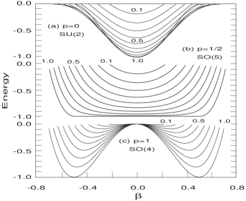
Figure 2: Coherent state energy surfaces. The energy units are $G^{(0)}_{\rm{eff}}\Omega^{2}/4$ for figures (a) and (b), and $\chi_{\rm{eff}}\Omega^{2}/4$ for (c). $H_{0}$ is taken as the energy zero point. Numbers on curves are the effective lattice occupation fractions, with $n/\Omega=1$ corresponding to half filling and $0<n/\Omega<1$ to finite hole doping. SO(5) symmetry corresponds to $p=1/2$ and the allowed range of $\beta$ is $[-\frac{1}{2}\sqrt{n/\Omega},\frac{1}{2}\sqrt{n/\Omega}]$, which depends on $n$.

With all the expectation values expressed in the coherent state representation, one can calculate the total energy. In Fig. 2, we show the coherent-state energy surfaces as a function of the order parameter $\beta$ for different electron occupation fractions $n/\Omega$ with $p=0,{1\over 2}$, and 1. The order parameter $\beta$ is related to the order parameter $Q\equiv\langle{\cal Q}_{z}\rangle$ and the electron number $n$ through $\langle{\cal Q}_{z}\rangle=2\Omega\beta\sqrt{n/2\Omega-\beta^{2}}$. For $p=0$ [SU(2) limit; see Fig. 2(a)], the minimum energy occurs at $\beta=0$ for all values of $n$, indicating SC order. For $p=1$ [SO(4) limit; see Fig. 2(c)], the opposite situation occurs: $\beta=0$ is an unstable point and energy minima lie at $\beta=\pm{1\over 2}\sqrt{n/\Omega}$, indicating the presence of AF order.

From Fig. 2(b), the SO(5) dynamical symmetry (with $p={1\over 2}$) is seen to have extremely interesting behavior: the minimum energy occurs at $\beta=0$ for all values of $n$, as in the SU(2) case, but there are large-amplitude fluctuations in $\beta$. In particular, when $n$ is near $\Omega$ (half filling), the system has an energy surface almost flat for broad ranges of $\beta$. This suggests a phase very soft against fluctuations in the order parameters. As $n/\Omega$ decreases, the fluctuations become smaller and the energy surface tends more and more to the SU(2) SC limit.

A symmetry limit having such a nature is termed a transitional or critical dynamical symmetry su4b ; wmzha88 . A critical dynamical symmetry is a dynamical symmetry having eigenstates that vary smoothly with a parameter (usually particle-number related) such that the eigenstates approximate one phase of the theory on one end of the parameter range and a different phase of the theory at the other end of the parameter range, with eigenstates in between exhibiting large softness against fluctuations in the order parameters describing the two phases. Thus, we believe that the rich physics in cuprates, in particular in the underdoped regime, must lie near the SO(5) limit, subject to a constraint by the parent SU(4) symmetry.

IV.3 SO(5) symmetry breaking

Under exact SO(5) symmetry ($p={\frac{1}{2}}$), the AF and SC states are degenerate at half filling. There is no barrier between AF and SC states, and one can fluctuate into the other at zero cost in energy (see the $n/\Omega=1$ curve of Fig. 2(b)). This situation is inconsistent with Mott insulating behavior at half-filling. The Zhang SO(5) model has been challenged because under exact symmetry it does not fully respect the phenomenological requirements of “Mottness”. As Zhang Zh97 has recognized, for antiferromagnetic insulator properties to exist at half filling, it is necessary to break SO(5) symmetry. Such breaking of the SO(5) subgroup symmetry is implicit in the SU(4) model, occurring naturally in the SU(4) model if $p>1/2$ in the Hamiltonian (9). Furthermore, the SU(4) symmetry leads to the following constraint

$$\langle{\cal E}_{su4}\rangle=\langle D^{\dagger}D+\vec{\cal Q}\cdot\vec{\cal Q}+\vec{\pi}\cdot\vec{\pi}\rangle=\mbox{$\small\frac{1}{4}$}\Omega^{2}(1-x^{2}),$$ (18)

which ensures a doping dependence in the solutions. Thus, the coherent state analysis indicates that the phenomenologically required SO(5) symmetry breaking and the doping dependence in the solutions occur naturally in the SU(4) model.

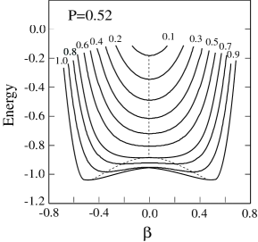
Figure 3: Coherent state energy surfaces for slightly perturbed SO(5). The dotted line indicates the location of the ground state as $n$ varies and the corresponding $\beta$ value where the energy curves have a minimum.

To see how in the SU(4) model a broken SO(5) symmetry can interpolate between AF and SC states as particle number varies, let us perturb slightly away from the SO(5) limit of $p={1\over 2}$. In Fig. 3, SU(4) coherent state results for $p=0.52$ are shown. One sees from Fig. 3 that if $n$ is near half filling ($n/\Omega=1$), $\beta_{\rm min}=\pm 0.5$; this corresponds to AF order, since the staggered magnetization reaches its maximum, $Q=\Omega/2$, and there are no pairing. With the onset of hole doping, $n/\Omega$ decreases (x increases). The AF correlation $Q$ quickly diminishes and the pairing correlations increase.

The SO(5) symmetry breaking in the Hamiltonian ($p>{1\over 2}$) is crucial. Only when SO(5) is broken does the energy surface interpolate between AF and SC order as doping is varied (compare the surfaces for $p=1/2$ and $p=0.52$ in Figs. 2(b) and 3). We thus conclude that high temperature superconductivity may be described by a Hamiltonian that conserves SU(4) but breaks (explicitly) SO(5) symmetry in a direction favoring AF order over SC order.

V Gap diagram at T$=$0

We have shown that with the coherent state method, one is able to calculate analytically all the physical quantities at and away from the symmetry limits. This provides a simple framework to study in more detail the observables. As our first application, we use the preceding results to study energy gaps in the cuprate systems at zero temperature.

V.1 The gap equations

We start from the symmetry-constrained variational Hamiltonian

$$H^{\prime}=H-\hat{n}\lambda+G{\cal E}_{su4},$$ (19)

where $H$ is the Hamiltonian (8), $\lambda$ and $G$ are two Lagrange multipliers determined by the constraints of number conservation, $\langle\hat{n}\rangle=n$, and conservation of the SU(4) invariant of Eq. (18).

Introducing the energy gaps

$$\Delta_{d}\equiv G^{\prime}_{0}\sqrt{\left\langle D^{\dagger}D\right\rangle}\qquad\Delta_{\pi}\equiv G^{\prime}_{1}\sqrt{\left\langle\vec{\pi}^{\dagger}\cdot\vec{\pi}\right\rangle}\qquad\Delta_{q}\equiv\chi^{\prime}\sqrt{\left\langle\vec{\cal Q}\cdot\vec{\cal Q}\right\rangle},$$ (20)

where we define

$$G^{\prime}_{0}\equiv G_{0}-G\qquad G^{\prime}_{1}\equiv G_{1}-G\qquad\chi^{\prime}\equiv\chi-G,$$

one obtains

$$\langle H^{\prime}\rangle=(\varepsilon-\lambda)n-\left(\ \frac{\Delta_{d}^{2}}{G^{\prime}_{0}}+\frac{\Delta_{\pi}^{2}}{G^{\prime}_{1}}+\frac{\Delta_{q}^{2}}{\chi^{\prime}}\ \right).$$ (21)

Variation of $\langle H^{\prime}\rangle$ with respect to $u_{\pm}$ or $v_{\pm}$ (that is, solving $\delta\langle H^{\prime}\rangle=0$) yields

$$2u_{\pm}v_{\pm}(\varepsilon_{\pm}-\lambda)-\Delta_{\pm}(u^{2}_{\pm}-v^{2}_{\pm})=0,$$

which is satisfied by

$$u^{2}_{\pm}=\frac{1}{2}\left(1+\frac{\varepsilon_{\pm}-\lambda}{e_{\pm}}\right)\qquad\displaystyle v^{2}_{\pm}=\frac{1}{2}\left(1-\frac{\varepsilon_{\pm}-\lambda}{e_{\pm}}\right),$$ (22)

with

$$e_{\pm}=\sqrt{(\varepsilon_{\pm}-\lambda)^{2}+{\Delta_{\pm}}^{2}}\qquad\Delta_{\pm}=|\Delta_{d}\pm\Delta_{\pi}|\qquad\varepsilon_{\pm}=\varepsilon\mp\Delta_{q}.$$ (23)

Inserting Eq. (22) into Eqs. (LABEL:eqone) and (18), and employing the gap definitions (20), one obtains the gap equations

$$\Delta_{d} = \frac{G^{\prime}_{0}\Omega}{4}\left(w_{+}\Delta_{+}+w_{-}\Delta_{-}\right)$$ (24)

$$\Delta_{\pi} = \frac{G^{\prime}_{1}\Omega}{4}\left(w_{+}\Delta_{+}-w_{-}\ \Delta_{-}\right)$$ (25)

$$\frac{4\Delta_{q}}{\chi^{\prime}\Omega} = w_{+}(\Delta_{q}+\lambda^{\prime})+w_{-}(\Delta_{q}-\lambda^{\prime})$$ (26)

$$-2x = w_{+}(\Delta_{q}+\lambda^{\prime})-w_{-}(\Delta_{q}-\lambda^{\prime})$$ (27)

$$\frac{1-x^{2}}{4}\Omega^{2} = \left(\frac{\Delta_{d}}{G^{\prime}_{0}}\right)^{2}+\left(\frac{\Delta_{\pi}}{G^{\prime}_{1}}\right)^{2}+\left(\frac{\Delta_{q}}{\chi^{\prime}}\right)^{2},$$ (28)

where

$$w_{\pm}\equiv\frac{1}{e_{\pm}},\qquad\lambda^{\prime}\equiv\lambda-\varepsilon\ .$$

By solving the above algebraic equations, all the gaps and the two Lagrange multipliers (the chemical potential $\lambda$ and the SU(4) correlation strength $G$) can be obtained. The three gaps $\Delta_{d}$, $\Delta_{\pi}$ and $\Delta_{q}$ represent, respectively, the energy scales of the singlet pairing, triplet pairing, and AF correlation, and we have introduced an analogous SU(4) gap $\Delta_{\rm SU4}$ to represent the energy scale of the SU(4) invariant through

$$\Delta_{SU4}\equiv G\sqrt{\left\langle{\cal E}_{\rm su4}\right\rangle}=\mbox{$\small\frac{1}{2}$}G\Omega\sqrt{1-x^{2}}.$$

Thus the ground state energy is determined by the four energy gaps (or energy scales)

$$E = \left\langle H^{\prime}\right\rangle+n\lambda-\mbox{$\small\frac{1}{4}$}G(1-x^{2})\Omega^{2}$$

$$= n\varepsilon-\left(\frac{\Delta_{SU4}^{2}}{G}+\frac{\Delta_{d}^{2}}{G^{\prime}_{0}}+\frac{\Delta_{\pi}^{2}}{G^{\prime}_{1}}+\frac{\Delta_{q}^{2}}{\chi^{\prime}}\right),$$

where $\left\langle H^{\prime}\right\rangle$ is given by Eq. (21). Once the gaps and the chemical potential $\lambda^{\prime}$ are known, the quasiparticle energies $e_{\pm}$, and the amplitudes $u_{\pm}$ and $v_{\pm}$, can all be determined through Eqs. (22)–(23), permitting other ground state properties to be calculated.

These results are in many respects analogous to the BCS theory with $v_{\pm}^{2}$ the probability of single particle level $\epsilon_{r\pm}$ being occupied, $\Delta_{\pm}$ the energy gap, and $e_{\pm}$ the quasiparticle energies. The essential difference is that conventional pairing theories deal with one pairing gap and one kind of quasiparticles; here we have two pairing energy gaps and two kinds of interacting quasiparticles, implying a larger variety of possible behavior. The quantities $e_{\pm}$ are two kinds of quasiparticle excitation energies, corresponding to two sets of nondegenerate single particle energy spectra $\{\varepsilon_{\pm}\}$ separated by $2\Delta_{q}$. Each level can be occupied by only one electron of either spin up or spin down. The corresponding pairing gaps are $\Delta_{\pm}$, the probabilities of single-particle levels being unoccupied are $u^{2}_{\pm}$, and the probabilities of single-particle levels being occupied are $v^{2}_{\pm}$.

V.2 Solution of gap equations at T$=$0

There are three parameters, $\chi$, $G_{0}$, and $G_{1}$, in the coupled algebraic equations (24)–(28), corresponding to the three elementary interactions in the SU(4) model: the AF correlation ($\chi$), the spin-singlet pairing ($G_{0}$), and the spin-triplet pairing ($G_{1}$). Physical solutions of the gap equations depend on the choices for these parameters. Experimental evidence suggests that these three interactions in the cuprate system are all attractive, and as demonstrated in Ref. su4d , $\chi$ should be the strongest and $G_{1}$ the weakest. Detailed analysis indicates su4d that SU(4) symmetric solutions exist only when $G=G_{1}$ (that is, when $G^{\prime}_{1}=0$). Thus, in the results presented below we shall assume the conditions

$$\chi\geq G_{0}\geq G_{1}\geq 0\qquad G=G_{1}$$

for the physical coupling constants. By solving Eqs. (24–28), analytical solutions for the gap equations at temperature $T=0$ can be obtained. Because of $G=G_{1}$, $\Delta_{\pi}$ is zero for any doping $x$, and the SU(4) gap is

$$\Delta_{\rm SU4}=\mbox{$\small\frac{1}{2}$}G_{1}\Omega\sqrt{1-x^{2}}.$$ (29)

Solution of other gaps at $T=0$ indicates that there is a critical doping point

$$x_{q}=\sqrt{\frac{\chi-G_{0}}{\chi-G_{1}}}=\sqrt{1-\frac{G^{\prime}_{0}}{\chi^{\prime}}}$$ (30)

separating qualitatively distinct solutions for the quasiparticle equations. When $x>x_{q}$, there exists a pure pairing state [all gaps entering Eqs. (24)–(28) except the singlet pairing gap $\Delta_{d}$ vanish]. When $x\leq x_{q}$, the gap equations have two solutions: the pairing solution remains but it is an excited state; another solution becomes the ground state, which differs from the pure pairing state by having both the AF gap $\Delta_{q}$ and the pairing gap $\Delta_{d}$ nonzero, and becoming a pure AF state at half filling. Specifically, one finds that for $x\leq x_{q}$

$$\Delta_{q} = \frac{\chi^{\prime}\Omega}{2}\sqrt{(x^{-1}_{q}-x)(x_{q}-x)}$$ (31)

$$\Delta_{d} = \frac{G^{\prime}_{0}\Omega}{2}\sqrt{x(x_{q}^{-1}-x)}$$ (32)

$$\lambda^{\prime} = -\frac{\chi^{\prime}\Omega}{2}x_{q}(1-x_{q}x),$$ (33)

while for $0<x\leq 1$ (but this is the ground-state solution only for $x>x_{q}$),

$$\Delta_{q} = 0$$ (34)

$$\Delta_{0}\equiv\Delta_{d} = \frac{G^{\prime}_{0}\Omega}{2}\sqrt{(1-x^{2})}$$ (35)

$$\lambda^{\prime} = -\frac{G^{\prime}_{0}\Omega}{2}x.$$ (36)

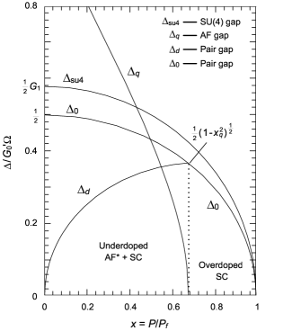
Figure 4: A generic gap diagram for energy gaps versus doping, as predicted by the SU(4) model. The energy gaps are scaled by the strength of the pairing correlation $G_{0}^{\prime}$ and the doping is scaled by the maximum doping P_f. The critical point $x_{q}$ = 0.68 is chosen in this plot and $\chi^{\prime}=17$, $G_{0}^{\prime}=8.2$, and $G_{1}=9.5$.

A generic gap diagram at $T=0$ describing features of the energy gaps as functions of the doping $x$ is shown in Fig. 4. The diagram is constructed using the analytical expressions (29, 31, 32, 34, 35). It is generic because the relative size of the gaps can be modified by the choice of interaction strengths but their basic forms are dictated entirely by the algebraic structure of the model. Four energy gaps are predicted:

1. The gap $\Delta_{q}$ measuring antiferromagnetic correlations (see Eq. (31)), which has its maximal value at $x=0$, decreases nearly linearly to the region of the pairing gaps as doping increases, crosses the pairing gaps, and vanishes eventually at the critical doping $x_{q}$.

2. The spin-singlet pairing gap $\Delta_{d}$ (see Eq. (32)), which is the superconducting gap for $x<x_{q}$. Starting from the critical doping $x_{q}$, it decreases as the doping decreases.

3. The spin-singlet pairing gap $\Delta_{0}=\Delta_{d}$ (see Eq. (35)), which is the superconducting gap for $x>x_{q}$ but is not the order parameter for the ground state in the doping range $x<x_{q}$. In $x<x_{q}$, it increases as the doping decreases.

4. The total SU(4) correlation measured by $\Delta_{\rm SU4}$, which has its doping dependence following Eq. (29) in the whole doping range.

It is interesting to observe that at the critical doping value $x_{q}$ the pairing gaps exhibit non-trivial behavior: for $x\geq x_{q}$, the singlet pairing gap corresponds to a single curve, labeled by $\Delta_{0}$. However, as the doping decreases from $x_{q}$, the energy scale $\Delta_{0}$ splits into two curves (labeled $\Delta_{d}$ and $\Delta_{0}$) having very different doping dependence.

V.3 Nature of the pseudogaps in cuprates

The qualitative features of the SU(4) gap diagram in Fig. 4 seem to agree well with many recent observations in cuprates Shen03 . In particular, the appearance of a quantum critical point $x_{q}$, the splitting of the pairing gap in the underdoped regime, and the existence of two distinct pseudogaps are basic predictions of the SU(4) model that have some experimental support.

The occurrence of the doping critical point and the splitting of the pairing gap below the critical point are understood in the SU(4) model as a direct consequence of the competing pairing and AF correlations below $x_{q}$. In this picture, the critical doping point $x_{q}$ defines a natural boundary between overdoped and underdoped regimes. It corresponds to the disappearance of AF correlations and separates a doping regime characterized by weak superconductivity and reduced pair condensation energy from a doping regime characterized by strong superconductivity and maximal pair condensation energy.

The origin of pseudogaps is one of the unsolved major problems in high-$T_{\rm c}$ superconductor physics. The pseudogap is believed to have a profound effect on a wide range of physical properties of cuprates and is generally considered to be intimately connected with the origins of high-temperature superconductivity. As noted in Refs. Shen03 , there is as yet little consensus about their origin and behavior but many proposed explanations fall into one of two categories: the preformed pair picture EK95 or the competing order picture Tallon01 . As we now briefly discuss (more detail will be published elsewhere su4d ), the SU(4) model predicts, and unifies at the microscopic level, two sources for pseudogap behavior, one of which may be interpreted as arising from preformed pairs and one of which may be interpreted as arising from competing order.

The preformed pair picture EK95 suggests that the pseudogap is the energy that is needed to form pairs as a first step in condensing them into a state with long-range order. A pseudogap arising in this way would be expected to decrease with increased doping and should merge with the pairing gap in the overdoped region. The SU(4) gap $\Delta_{\rm SU(4)}$ has exactly these properties. As can be seen from Eq. (29), $\Delta_{\rm SU(4)}$ depends only on $G_{1}$ and is independent of $x_{q}$. It is maximal at half-filling and falls to zero at the largest doping. This gap is related to the SU(4) invariant ${\cal E}_{\rm su4}$ (see Eq. (18)), which is state independent. Therefore, the SU(4) gap is expected to have no temperature dependence, as long as the SU(4) symmetry is preserved.

On the other hand, the competing order picture Tallon01 suggests that the pseudogap is the energy scale for some form of order competing with superconductivity. A pseudogap originating in competing order should not generally merge with the pairing gap and may fall to zero at a critical doping point where the competing order is completely suppressed relative to the superconducting order. The SU(4) antiferromagnetic gap $\Delta_{q}$ has these properties and gives rise to a pseudogap that may be interpreted in terms of competing AF and SC order. Specifically, the scale $\Delta_{q}$ is the energy per electron required to break the AF correlation and serves as an order parameter of the AF phase.

Thus, the SU(4) model predicts the existence of two distinct pseudogaps. The seemingly rather contradictory mechanisms for the origin of the pseudogaps as suggested in Refs. EK95 ; Tallon01 may find a consistent explanation in the SU(4) model.

VI Conclusion

The SU(4) symmetry represents a fully microscopic fermion system in which SC and AF modes enter on an equal footing. At this “unification” level, there is in a sense no distinction among these degrees of freedom, just as in the Standard Electroweak Theory of elementary particle physics the electromagnetic and weak interactions are unified above the intermediate vector boson mass scale. We may view the system as having condensed into SU(4) pairs, which fixes the length of the state vectors (through the SU(4) Casimir expectation value) but not their direction in the state-vector space. Physically, this means that the system is paired, with the pair structure exhibiting SU(4) symmetry, but is neither SC nor AF because fluctuations on a scale set by the temperature prevent selection of the SC or AF directions. Stated in another way, the SU(4) pairs are of collective strength, but are not condensed into a state with long-range order. Stated in yet another way, neither the AF nor SC order parameters have finite expectation values in this regime, but a sum of their squares (the SU(4) Casimir) does. This constraint implies an intimate connection between superconductivity and antiferromagnetism in the SU(4) model. They are, in a sense, different projections of the same fundamental vector in an abstract algebraic space.

Compared to the Hubbard or t-J models, the dynamical symmetry approach applied here represents a different way to simplify a strongly-correlated many-body problem. In the Hubbard or t-J models, approximations are made to simplify the Hamiltonian but no specific truncation is assumed for the configuration space, although in practical calculations a truncation is typically necessary. In contrast, we make no approximation to the Hamiltonian. The only approximation is the (severe) space truncation. The symmetry dictated Hamiltonian includes all possible interactions in the truncated space. In principle, if all the degrees of freedom of the system are included, this approach constitutes an exact microscopic theory. The validity of this approach depends entirely on the validity of the choice of truncated space, which may be tested by comparison with the data.

The advantage of the dynamical symmetry approach is its cleanness and simplicity. It is clean because the only approximation is the selection of the truncated model space. Thus, a failure of the method is a strong signal that one has chosen a poor model space. It is simple because the method supplies analytical solutions for various dynamical symmetry limits as a starting point. These symmetry-limit solutions provide an immediate handle on the physics and permit an initial judgement of the model’s validity without large-scale numerical calculations. Beyond the symmetry limits, numerical calculations may be necessary. However, because of the low dimensionality of the models spaces and the power of group theory, such numerical calculations are much simpler than those in, say, a Hubbard or t-J model.

Simple symmetries as a predictor of dynamics has found powerful application in fields such as particle physics or nuclear physics. Although a real physical system may be very complex, these applications are based on the obvious point that nature has managed to construct a stable ground state having well-defined collective properties that change systematically from compound to compound. Extensive experience in many fields of physics suggests that this is the signal that the phenomenon in question is described by a small effective subspace with renormalized interactions (that may differ substantially in form and strength from those of the full space) and governed by a symmetry structure of manageable dimensionality. The results described here suggest that the observational complexities of high temperature superconductors may also be described by a simple theory based on dynamical symmetries having these properties.