Local density of states at polygonal boundaries of $d$-wave superconductors

Abstract

Besides the well-known existence of Andreev bound states, the zero-energy local density of states at the boundary of a $d$-wave superconductor strongly depends on the boundary geometry itself. In this work, we examine the influence of both a simple wedge-shaped boundary geometry and a more complicated polygonal or faceted boundary structure on the local density of states. For a wedge-shaped boundary geometry, we find oscillations of the zero-energy density of states in the corner of the wedge, depending on the opening angle of the wedge. Furthermore, we study the influence of a single Abrikosov vortex situated near a boundary, which is of either macroscopic or microscopic roughness.

I Introduction

The local density of states at the boundary of a superconductor is a crucial factor in many experiments, for example tunneling measurements. For conventional $s$-wave superconductors, the local density of states at an insulating boundary is practically the same as in the bulk. In particular, the specific boundary geometry is irrelevant. In the case of $d$-wave symmetry, however, the situation is completely different. Due to Andreev bound states Hu ; Tanaka ; Buchholtz , a drastic enhancement of the low-energy density of states can be observed at a straight flat surface appearing as a pronounced zero-bias conductance peak Iguchi ; Lesueur ; Covington . This effect is maximal if the $d$-wave nodal direction is perpendicular to the boundary and shrinks when the orientation is changed Tanaka ; Iguchi . For an angle of 45 degrees between nodal direction and boundary, the Andreev bound states disappear completely. Besides this well-known effect, it is important to realize that for $d$-wave symmetry also the boundary geometry itself can have strong influence on the local density of states. In this work we examine the local density of states at the surface of a $d$-wave superconductor for some basic examples of polygonal boundary geometries and show that Andreev bound states are sensitive to the boundary geometry. We also consider the additional influence of a single Abrikosov vortex pinned near the boundary.

In a previous work we have shown, that the presence of an Abrikosov vortex in the vicinity of the boundary of a $d$-wave superconductor has a drastic effect on the zero-energy Andreev bound states. This effect appears as a surprisingly large shadow-like suppression of the zero-energy density of states between vortex and boundary ShadowPRL . The suppression is due to the supercurrent flowing around the vortex, which locally shifts the quasiparticle energies and leads to a splitting of the zero-energy peak. A similar splitting has already been studied for a homogeneous surface currentFogelstroem ; CovingtonAprili ; Aprili ; Dagan . One of the purposes of the present study is to show that this vortex shadow effect is stable and robust even if the boundary of the superconductor possesses some roughness or faceting.

The paper is divided into five sections. In the next section, we give a short introduction to the theoretical framework used for the calculations. In the third section, we present some zero-energy local densities of states for simple wedge-shaped boundary geometries and discuss some elementary effects. After that, we turn to the aspect of boundary roughness in section four, where we consider more complicated polygonal boundary structures. Finally, we end with our conclusions in section five.

II Theoretical background

II.1 The Riccati formalism

In the limit $k_{F}\xi\gg 1$, the equilibrium properties of a superconductor are contained in the Eilenberger propagator $\hat{g}(\vec{r},\vec{k}_{F},i\epsilon_{n})$. The propagator itself can be calculated by solving a transport-like equation first introduced by Eilenberger Eilenberger and independently by Larkin and Ovchinnikov Larkin . Here, we will use the so-called Riccati parametrization of the Eilenberger theory, which was introduced in Ref. SchopohlMaki, and has proven to be very useful for the numerical computation of the propagator (for more details see Ref. DGIS, ). In order to obtain a solution for a given Fermi vector $\vec{k}_{F}$ at the point $\vec{r}_{0}$, the coupled Eilenberger equations are parametrized along a trajectory passing through $\vec{r}_{0}$ in direction of the Fermi velocity corresponding to $\vec{k}_{F}$

$$\vec{r}(x)=\vec{r}_{0}+x\;\vec{v}_{F}(\vec{k}_{F})$$ (1)

Along this trajectory, the Eilenberger equations can be transformed to two decoupled differential equations of the Riccati type for the scalar functions $a(x)$ and $b(x)$:SchopohlMaki

$$\hbar v_{F}\partial_{x}a(x)+\left[2\epsilon_{n}+\Delta(x)^{*}a(x)\right]a(x)-\Delta(x) = 0$$

$$\hbar v_{F}\partial_{x}b(x)-\left[2\epsilon_{n}+\Delta(x)b(x)\right]b(x)+\Delta(x)^{*} = 0$$ (2)

Here, we have already removed the vector potential $\vec{A}(\vec{r})$ via a gauge transformation. This can be done for the case of a single pinned Abrikosov vortex in a high-$\kappa$ superconductor, since we concentrate on lengthscales smaller than the penetration depth $\lambda$. Together with the starting values in the bulk

$$a(-\infty)=\frac{\Delta(-\infty)}{\epsilon_{n}+\sqrt{\epsilon_{n}^{2}+|\Delta(-\infty)|^{2}}}$$

$$b(+\infty)=\frac{\Delta^{*}(+\infty)}{\epsilon_{n}+\sqrt{\epsilon_{n}^{2}+|\Delta(+\infty)|^{2}}}$$ (3)

the functions $a$ and $b$ can be integrated in an easy and numerically stable way along the trajectory.

The Eilenberger propagator $\hat{g}$ is related to the functions $a$ and $b$ by

$$\hat{g}=\frac{-\pi i}{1+ab}\left(\begin{array}[]{cc}1-ab&2ia\\ -2ib&-1+ab\end{array}\right)$$ (4)

Assuming a cylindrical Fermi surface, $\vec{k}_{F}$ depends only on an polar angle $\theta$

$$\vec{k}_{F}=k_{F}\left(\begin{array}[]{c}\cos\theta\\ \sin\theta\end{array}\right)$$ (5)

and the local density of states, normalized to the normal state density of states at the Fermi level $N_{0}$, is given by

$$N(\vec{r}_{0},E)=\int_{0}^{2\pi}\frac{d\theta}{2\pi}{\rm Re}\;\left[\frac{1-ab}{1+ab}\right]_{i\epsilon_{n}\rightarrow E+i\delta}$$ (6)

Practically, this means that the integrand has to be evaluated for many angles $\theta$, each angle corresponding to one particular trajectory through $\vec{r}_{0}$. The energy $E$ is taken with respect to the Fermi level and $\delta$ can be regarded as an effective scattering parameter which is proportional to an inverse mean free path.

In the calculations presented below, the specific boundary geometry of the superconductor has to be taken into account. Since we assume that the transmission coefficient of all the boundaries is zero, the boundary conditionsZaitsev ; RainerBuchholtz ; Shelankov simplify considerably. In our case, a trajectory which hits the boundary is simply reflected like a ray of light. Thus, for the calculations in this work, a ray tracing procedure has been used, which allows for multiple specular reflections. The Riccati equations (2) then have to be solved on such a multiply reflected trajectory (see for example the trajectories in Fig. 5b)).

II.2 Model for the Gap function

We consider gap functions $\Delta(\vec{r},\vec{k}_{F})$ that can be separated into

$$\Delta(\vec{r},\vec{k}_{F})=\Delta_{0}\chi(\vec{k}_{F})\psi(\vec{r})$$ (7)

Here, the symmetry function for the $d_{x^{2}-y^{2}}$-wave is $\chi(\theta)=\cos(2\theta)$. In the following we want to concentrate on the part $\psi(\vec{r})$ of the gap function, which covers the spatial dependence. It can be factorized into modulus and phase

$$\psi(\vec{r})=f_{p}(\vec{r})e^{i\phi(\vec{r})}$$ (8)

where we call the modulus $f_{p}(\vec{r})$ the profile function. In principle, both the profile function and the phase $\phi(\vec{r})$ should be calculated selfconsistently via the gap equation. For simplicity, we have taken the profile function to be constant. This is a good approximation for low temperatures due to the Kramer-Pesch effect KramerPesch . Even for higher temperatures, the changes in the quasiparticle spectra due to this simplification are rather of a quantitative than a qualitative nature. Compared to the constant model profile function, the relevant differences of a more realistic profile function most often reside in comparatively small intervals along the trajectories. For the situation studied in the following, this occurs near the boundaries or close to the vortex center. In these regions, the local density of states is somewhat smeared out or softened, if a more realistic profile function is used. However, the main features to be presented below remain unaffected, as we have checked for specific situations.

In the absence of a vortex, the phase $\phi(\vec{r})$ of the gap function simply is zero. For the case of a pinned Abrikosov vortex in the system considered here, as an excellent approximation, the gradient of the phase is parallel to the current $\vec{j}(\vec{r})$

$$\vec{\nabla}\phi(\vec{r})\;||\;\vec{j}(\vec{r})$$ (9)

and $\phi(\vec{r})$ is given as a solution of the Laplace equation

$$(\partial^{2}_{x}+\partial^{2}_{y})\phi(\vec{r})=0$$ (10)

with a ”phase source” of $2\pi$ at the vortex position. In other words, integrating the phase gradient along any closed path around the vortex position must add up to a total of $2\pi$. Additionally, $\phi(\vec{r})$ has to fulfill von-Neumann boundary conditions

$$\partial_{n}\phi(\vec{r})=0$$ (11)

since currents are not allowed to cross any of the boundaries. Here, $\vec{n}$ denotes the normal vector of the boundary under consideration.

To solve the Laplace equation in two dimensions, we use the method of conformal mapping. This analytical technique can be found in many mathematical textbooks, and in some specific physical textbooks as well. Nevertheless, in the following we give the main aspects of conformal mapping in short. First, the original two-dimensional domain, where the solution of the Laplace equation is sought, is regarded as a part of the complex plane. This domain is also referred to as physical domain, and it often includes a nontrivial boundary geometry with specific boundary conditions. The main idea and task is to map this physical domain to a simple ”model” domain by using analytic functions. Because of the latter, the Laplace equation itself stays invariant under this mapping. Thus, if the solution of Laplace’s equation with the correct boundary conditions is known in the model domain, also the original problem is solved. The solution in the physical domain can then be achieved by simply mapping each point to the model domain with the mapping function and taking the corresponding value of the solution there.

In our case of a wedge-shaped physical domain, the upper complex half space serves as the model plane and $w,w_{V}$ shall denote elements thereof. Then, the function $\Phi$, which is given by the formula

$$\textrm{e}^{i\Phi}=\frac{w-w_{V}}{\left|w-w_{V}\right|}\cdot\frac{w^{*}-w_{V}}{\left|w^{*}-w_{V}\right|}$$ (12)

is the analytical solution of Laplace’s equation

$$\partial_{w}\partial_{w^{*}}\Phi=0$$ (13)

in all points $w$ of the upper half plane with $w\neq w_{V}$. Integrating the phase gradient around the singularity at $w=w_{V}$ results in a total phase difference of $2\pi$. Thus, $w_{V}$ can be regarded as the position of the phase vortex. Also, von-Neumann boundary conditions are satisfied, since the phase gradient is parallel to the boundary (the real axis). Of course, formula (12) is analogous to the well-known mirror image ansatz in electrostatics, the first factor referring to a vortex at position $w_{V}$, the second to a virtual antivortex at the mirrored position $w_{V}^{*}$.

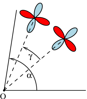
Figure 1: A $d_{x^{2}-y^{2}}$-wave superconductor with wedge-shaped boundary geometry. $\alpha$ denotes the opening angle of the wedge. The orientation between $d$-wave and wedge is parametrized by the angle $\gamma$, which gives the rotation of the full-gap direction with respect to the bisecting line of the wedge. The origin $O$ represents the corner of the wedge.

Since the correct solution of the problem in the model domain is given by (12), the next and also last step is to find an analytical function which maps the physical domain to the upper half plane. It is well-known that the complex power function is analytic and that

$$z(w)=w^{\frac{\alpha}{\pi}}$$ (14)

maps the upper half plane to a wedge with opening angle $\alpha$. In particular, the positive real axis is mapped onto itself. Thus, for the physical domain being a wedge with opening angle $\alpha$ measured from the positive real axis, the sought mapping function is just the inversion

$$w(z)=z^{\frac{\pi}{\alpha}}$$ (15)

However, this mapping function is only valid for $\alpha\leq\pi$. For opening angles $\pi\leq\alpha\leq 2\pi$ one has to be careful about the branch cut discontinuity at the negative real axis. A possible mapping is then given by

$$w(z)=\textrm{e}^{i\pi(1-\frac{\pi}{\alpha})}\left[z\textrm{e}^{i(\pi-\alpha)}\right]^{\frac{\pi}{\alpha}}$$ (16)

Finally, combining the solution (12) in the model plane with the above mapping functions $w(z)$, the phase factor of the gap function for a wedge-shaped boundary is given by

$$\textrm{e}^{i\phi(\vec{r})}=\frac{w(z)-w(z_{V})}{\left|w(z)-w(z_{V})\right|}\cdot\frac{w(z)^{*}-w(z_{V})}{\left|w(z)^{*}-w(z_{V})\right|}$$ (17)

On the right hand side, $z=r_{x}+ir_{y}$ is the position vector $\vec{r}$ in complex notation. Analogous, the position of the vortex can be chosen with the parameter $z_{V}=r_{V,x}+ir_{V,y}$. The opening angle $\alpha$ of the wedge enters via the mapping functions (15) or (16), respectively. In principle, the phase factor of more than one vortex is simply the product of several one-vortex solutions (17). However, in the following we will confine ourselves to the case of only one single vortex.

III Wedge-shaped boundary geometry

In this section, we investigate the zero-energy local density of states of $d_{x^{2}-y^{2}}$-wave superconductors with wedge-shaped boundary geometries. The situation is sketched in Fig. 1. $\alpha$ denotes the opening angle of the wedge, $\gamma$ the angle between the bisecting line of the wedge and the direction of the maximum gap. Some examples for wedges with opening angles $\alpha=\pi/2$ and $\alpha=\pi/4$ can be seen in Figs. 2 and 3. Far away from the corner, the zero-energy density of states at the boundaries exhibit the well-known Andreev bound states. If the nodal direction of the $d$-wave is perpendicular to the specific boundary line, a maximum value is reached (e.g. Fig. 2c), both boundaries, or 3a), upper boundary). For other orientations, the Andreev bound states are smaller (Fig. 2b) and 3b)), or they even vanish if the direction of the maximum gap is perpendicular to the boundary (e.g. Fig. 2a) or 3a), lower boundary). In all the calculations presented here and in the following sections, the effective scattering parameter is set to $\delta=0.1\Delta_{0}$. This leads to a nonzero value of the zero-energy density of states in the bulk and limits the absolute value of the Andreev bound states at the boundaries.

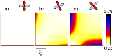
Figure 2: Zero-energy density of states of a $d_{x^{2}-y^{2}}$-wave superconductor for a wedge-shaped boundary with opening angle $\alpha=\pi/2$. The density of states is normalized to the density $N_{0}$ of the normal state. The effective scattering parameter is chosen to be $\delta=0.1\Delta_{0}$. The rotation of the $d$-wave with respect to the bisecting line is a) $\gamma=-\pi/4$, b) $\gamma=-\pi/8$, c) $\gamma=0$.

It is important to realize, however, that in a range from the corner, which is given by the lengthscale $\xi=\hbar v_{F}/\Delta_{0}$, the boundary geometry itself strongly influences the local density of states. A very counterintuitive example can be seen in Fig. 2c). Although the zero-energy local density of states reaches its maximum height along both boundary lines, the corner of the right-angled wedge itself only exhibits the bulk value of $0.23$. For the smaller opening angle $\alpha=\pi/4$, the local density of states in the tip of the wedge can even be lower than in the bulk: In Fig. 3b), where $\gamma=0$, which refers to a maximum gap direction parallel to the bisecting line, the value is $0.11$. This is barely larger than the bulk value corresponding to an $s$-wave superconductor.

By just taking a look at Figs. 2 and 3 one might get the impression, that the zero-energy density of states in the corner is always suppressed independently of the rotation angle $\gamma$ of the $d$-wave. However, this is not true in general. In Fig. 4 we examine a wedge with opening angle $\alpha=\pi/3$. We can clearly see that for the the nodal direction being parallel to the bisecting line ($\gamma=\pi/4$), there is a strong increase of the zero-energy local density of states in the corner.

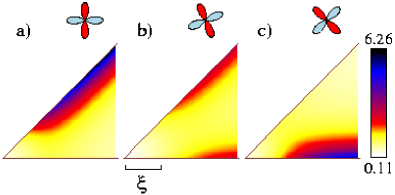
Figure 3: Zero-energy density of states of a $d_{x^{2}-y^{2}}$-wave superconductor for a wedge-shaped boundary with opening angle $\alpha=\pi/4$. The density of states is normalized to the density $N_{0}$ of the normal state. The effective scattering parameter is chosen to be $\delta=0.1\Delta_{0}$. The rotation of the $d$-wave with respect to the bisecting line is a) $\gamma=-\pi/8$, b) $\gamma=0$, c) $\gamma=\pi/8$.

III.1 Local density of states in the corner of the wedge

In the following, we want to concentrate on the corner point $O$ and systematically examine, why the local density of states seems to behave so strange.

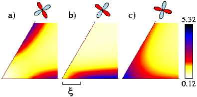
Figure 4: Zero-energy density of states of a $d_{x^{2}-y^{2}}$-wave superconductor for a wedge-shaped boundary with opening angle $\alpha=\pi/3$. The density of states is normalized to the density $N_{0}$ of the normal state. The effective scattering parameter is chosen to be $\delta=0.1\Delta_{0}$. The rotation of the $d$-wave with respect to the bisecting line is a) $\gamma=0$, b) $\gamma=\pi/8$, c) $\gamma=\pi/4$.

In Fig. 5a), the zero-energy local density of states in the corner is shown. The opening angle $\alpha$ of the wedge-shaped boundary geometry corresponds to the vertical axis. The rotation angle $\gamma$ of the $d$-wave is varied from $0$ to $\pi/2$ along the horizontal axis. The absolute maximum value is right in the center of the figure. Here, $\alpha=\pi$ and $\gamma=\pi/4$ correspond to the well-known maximum Andreev bound states at a straight boundary line. The most interesting part of the picture can be seen at smaller opening angles $\alpha\leq\pi$. If the nodal direction of the $d$-wave is kept fixed parallel to the bisecting line of the wedge (i.e. $\gamma=\pi/4$) and the opening angle $\alpha$ is reduced, then the zero-energy local density of states clearly oscillates between high maxima and minima. A cut along this line showing the oscillations in the range $0<\alpha\leq\pi/2$ is shown in Fig. 6. Clearly, the minima of the oscillating zero-energy local density of states in the corner appear for opening angles $\alpha^{+}_{n}=\pi/(2n)$, while the maxima are very close to the angles $\alpha^{-}_{n}=\pi/(2n-1)$.

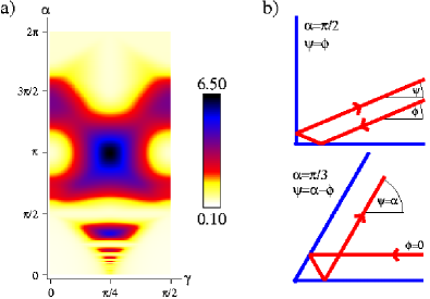
Figure 5: a) Zero-energy density of states in the corner $O$ of a $d_{x^{2}-y^{2}}$-wave superconductor with wedge-shaped boundary geometry. $\alpha$ denotes the opening angle of the wedge, $\gamma$ the rotation of the maximum gap direction with respect to the bisecting line of the wedge. The global maximum in the middle of the picture corresponds to the well-known maximum of the Andreev bound states at a straight boundary line, with the nodal direction of the $d$-wave being perpendicular to the boundary. b) Two examples for the relations (18) and (19). The upper panel shows, that for an opening angle of $\alpha=\pi/2$ an incoming trajectory always leaves the corner at the same angle. For an opening angle of $\alpha=\pi/3$, the directions of the incoming and outgoing trajectories are symmetric with respect to the bisecting line of the wedge (lower panel).

III.2 Explanation of the oscillations

For opening angles $\alpha<\pi$, multiple reflections of a quasiparticle trajectory occur, because the boundaries are hit several times. Generally, for a given opening angle $\alpha$, the exact path of a quasiparticle trajectory has to be determined by a raytracing algorithm. However, there are some specific opening angles $\alpha_{n}=\pi/n$, which have useful properties and are the key in understanding the oscillations. We denote $\phi\in\left[0,\alpha\right]$ the angle of an incoming trajectory before any reflection has occured, and call $\psi\in\left[0,\alpha\right]$ the angle of the final outgoing trajectory after all the multiple reflections. Then, the specific opening angles $\alpha_{n}^{+}=\pi/(2n)$ have the property, that always

$$\psi=\phi$$ (18)

while for $\alpha_{n}^{-}=\pi/(2n-1)$ we always have

$$\psi=\alpha-\phi$$ (19)

In the first case, incoming and outgoing trajectories are parallel. This means that the gap value is the same on the incoming and outgoing part of the trajectory. In contrast, in the second case the angles of incoming and outgoing trajectories are symmetric with respect to the bisecting line of the wedge. For $\gamma=\pi/4$ (nodal direction along the bisecting line) this means, that the gap possesses opposite sign on the incoming and outgoing part of the trajectory, which results in large contributions to the zero-energy density of states in the corner. Two typical examples for the different symmetry behaviour of in- and outgoing trajectory directions are shown in Fig. 5b).

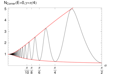
Figure 6: Oscillation of the zero-energy density of states in the corner $O$ of a $d_{x^{2}-y^{2}}$-wave superconductor with wedge-shaped boundary geometry. The nodal direction of the $d$-wave is fixed parallel to the bisecting line of the wedge, i.e. $\gamma=\pi/4$. Decreasing the opening angle $\alpha$ leads to oscillations of the density of states in the corner, with minima appearing at $\alpha^{+}_{n}=\pi/(2n)$ and maxima close to $\alpha^{-}_{n}=\pi/(2n-1)$. Both upper and lower envelope (dotted lines) are given analytically.

Now we turn to the calculation of the local density of states in the corner point $O$ of the wedge. For the trajectories passing through this point, it is an excellent assumption to neglect all the complicated details of the multiple reflections in the corner completely, since they occur on a very small lengthscale along the trajectory path. The only important things to keep are the relations between the angles of incoming and finally outgoing trajectories. Thus, the effect of the wedge-shaped boundary geometry is only a mixing of the bulk values (3) of $a$ and $b$ belonging to different angles. If we concentrate on the specific opening angles $\alpha_{n}$ with the relations (18) and (19), it is possible to derive an analytic expression for the local density of states in the corner.

The oscillations in Fig. 6 appear for the $d$-wave orientation $\gamma=\pi/4$, where the nodal direction is parallel to the bisecting line of the wedge. Based on relation (18) for opening angles $\alpha_{n}^{+}=\pi/(2n)$, we find the lower envelope

$$N_{\textrm{Corner}}^{+}(E=0,\gamma=\pi/4)$$

$$= \frac{1}{\alpha}\int_{-\alpha/2}^{\alpha/2}d\phi\frac{1}{\sqrt{1+\frac{\Delta_{0}^{2}}{\delta^{2}}\sin^{2}2\phi}}=\frac{1}{\alpha}F(\alpha,-\Delta_{0}^{2}/\delta^{2})$$

Analogous, the upper envelope, which connects the values of the local density of states for opening angles $\alpha_{n}^{-}=\pi/(2n-1)$, is given by

$$N_{\textrm{Corner}}^{-}(E=0,\gamma=\pi/4)$$

$$= \frac{1}{\alpha}\int_{-\alpha/2}^{\alpha/2}d\phi\sqrt{1+\frac{\Delta_{0}^{2}}{\delta^{2}}\sin^{2}2\phi}=\frac{1}{\alpha}E(\alpha,-\Delta_{0}^{2}/\delta^{2})$$

Here, $F$ and $E$ are Elliptic Integrals of the First and Second Kind. Both upper and lower envelope are shown as the dotted lines in Fig. 6. As already mentioned before, we chose the effective scattering parameter $\delta=0.1\Delta_{0}$. For the lower envelope, all the bulk values stemming from an interval of length $\alpha$ around the nodal line contribute to the local density of states in the corner. Because of that, for $\alpha=\pi/2$ the whole quasiparticle spectrum in the corner is the same as in the bulk, since contributions from the full $d$-wave are included. In particular, the zero-energy density of states in the corner is just the bulk value. When the opening angle $\alpha$ is reduced, however, the result approaches the normal state value $1$. The upper envelope is dominated by bound states, which occur by the mixing due to relation (19), since the gap function changes sign at the bisecting line of the wedge. The highest contribution to the bound states is confined by the opening angle $\alpha$. Thus, after the maximum for $\alpha=\pi$ at the flat boundary, the upper envelope shrinks to the normal state value $1$ for smaller opening angles.

If the maximum gap direction of the $d$-wave is parallel to the bisecting line of the wedge, i.e. $\gamma=0$, the sign of the gap function is symmetric with respect to the bisecting line. Then, the mixing (19) of the specific opening angles $\alpha_{n}^{-}$ generates nothing but bulk contributions, too. Consequently, for all the opening angles $\alpha_{n}=\pi/n$, no bound states appear at all. The corresponding values of the zero-energy local densities of states in the corner are on the same curve for both $\alpha_{n}^{+}$ and $\alpha_{n}^{-}$:

$$N_{\textrm{Corner}}(E=0,\gamma=0)=\frac{1}{\alpha}\int_{-\alpha/2}^{\alpha/2}d\phi\frac{1}{\sqrt{1+\frac{\Delta_{0}^{2}}{\delta^{2}}\cos^{2}2\phi}}$$ (22)

$$= \frac{\frac{\delta}{\Delta_{0}}}{\sqrt{\frac{\delta^{2}}{\Delta_{0}^{2}}+1}}\frac{1}{\alpha}F(\alpha,1/(1+\delta^{2}/\Delta_{0}^{2}))$$

For $\alpha_{1}=\pi$ and again for $\alpha_{2}=\pi/2$, we have the same density of states both in the bulk and in the corner. For smaller opening angles, only the contributions from the full-gap direction remain. The local density of states in the corner approaches the shape of a bulk $s$-wave spectrum. Because of that, the zero-energy weight approaches the $s$-wave bulk value, as already pointed out before. Although there are no zero-energy bound states in the corner of the wedge for the specific opening angles $\alpha_{n}=\pi/n$, multiple reflections lead to considerable bound states for angles $\pi/2<\alpha<\pi$. For arbitrary opening angles $\alpha<\pi/2$, however, the deviation of the zero-energy density of states in the corner from Eq. (22) determined by the $\alpha_{n}$ is small.

To summarize this section: Whether Andreev bound states appear in the corner of a wedge or not depends on both opening angle $\alpha$ of the wedge and orientation $\gamma$ of the $d$-wave. For $\alpha<\pi/2$, Andreev bound states in the corner are suppressed in most of the parameter space. However, near the specific opening angles $\alpha_{n}^{-}=\pi/(2n-1)$ and for orientations about $\gamma=\pi/4$, Andreev bound states get induced in the corner. Fig. 5a) provides a map, showing for which combinations of angles Andreev bound states appear.

III.3 Wedge and Vortex

We already discussed the influence of a single Abrikosov vortex, which is pinned near a straight smooth boundary, on the local quasiparticle spectrum in a previous work ShadowPRL . The result is a suppression of the zero-energy Andreev bound states in a shadow-like region extending from the vortex to the boundary. This effect is due to the flow field of the phase gradient around the vortex, which leads to a local shift of the quasiparticle energy along the trajectory. As a consequence, the zero-energy Andreev bound states at the boundary are suppressed and the spectral weight is shifted towards higher quasiparticle energies as discussed in Ref. ShadowPRL, .

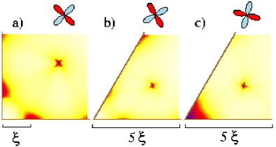
Figure 7: Zero-energy density of states of $d_{x^{2}-y^{2}}$-wave superconductors with wedge-shaped boundary geometries. A single Abrikosov vortex is pinned at a distance of 2 $\xi$ from each boundary line. All pictures presented here correspond to a specific wedge and orientation already shown earlier without a vortex. The same color palettes have been used for both the corresponding plot without vortex and the plot given here. a) This picture refers to Fig. 2c). The vortex casts a shadow-like suppression on the Andreev bound states at each boundary. b) This picture refers to Fig. 4a). Again, the Andreev bound states at the boundaries are locally suppressed. c) This picture refers to Fig. 4c). The bound states in the corner induced by the boundary geometry are also affected but remain still considerable. Please note, that b) and c) are given in a smaller scale than the corresponding pictures.

Some examples of a single Abrikosov vortex, which is pinned near a wedge-shaped boundary geometry, are shown in Fig. 7. Here, we have calculated the phase distribution around the vortex using the conformal mapping procedure described in section II B. Each picture corresponds to a picture with the same wedge geometry and $d$-wave orientation already presented in earlier figures. As a main effect, the existence of the vortex and its inhomogeneous phase lead to a local suppression of the zero-energy Andreev bound states at the boundaries. The center of the suppression seems to be approximately that point of the boundary, which lies closest to the vortex.

If we concentrate on the very corner of the wedge, however, the characteristic changes of the local density of states induced by the boundary geometry itself are only slightly affected by the presence of the vortex. Of course, the induced bound states in the corner of Fig. 4c), for example, get reduced by about 30 % in Fig. 7c) because of the vortex. Nevertheless, the zero-energy density of states is still strongly increased in the corner compared to the bound states at the boundary nearby. An induced suppression of the zero-energy density of states in the corner is practically not affected by the vortex as can be seen in Figs. 7a) and b). It is important to realize, however, that the shown suppressions of the zero-energy local density of states are not of the same nature. On the one hand, the suppression due to the vortex is the result of a splitting of the sharp zero-energy peak in the quasiparticle spectrum. On the other hand, the low value of the zero-energy density of states because of the boundary geometry is just a natural consequence, when the quasiparticle spectrum in the corner is given by a $d$- or even $s$-wave bulk spectrum.

Some further examples of a wedge with opening angle $\alpha=3\pi/2$ and an Abrikosov vortex at different positions can be seen in Fig. 8. In the top row, the shadow effect can be observed again. Below, there are no bound states at the boundaries at all, and the influence of the vortex rather leads to a very small increase of the zero-energy density of states.

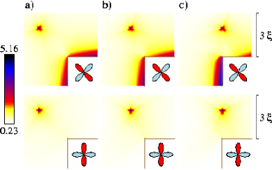
Figure 8: Zero-energy density of states of a $d_{x^{2}-y^{2}}$-wave superconductor for a wedge-shaped boundary with opening angle $\alpha=3\pi/2$. A single Abrikosov vortex is situated at a vertical distance of $2\xi$ from the corner of the wedge. The horizontal distance of the vortex is a) $2\xi$, b) $\xi$, c) 0. In the top row, the nodal direction of the $d$-wave is perpendicular to both boundaries, which corresponds to $\gamma=0$. Below, the nodal direction is parallel to the bisecting line, i.e. $\gamma=\pi/4$.

IV Polygonal boundary structure

In this section, we want to study the influence of surface roughness and surface faceting on the vortex shadow effect introduced in Ref. ShadowPRL, in order to see how stable this effect is. There have been several different suggestions in the literature how surface roughness can be implemented within Eilenberger theory (see for example Refs. Shelankov, ; Fogelstroem, ; Thuneberg, ). Here, we focus on the zero-energy density of states in the vicinity of a boundary line for two different models of either microscopic or macroscopic roughness with respect to the lengthscale of the coherence length. We begin with a very simple model of microscopic roughness in the next subsection. After that, we present results for a polygonal boundary structure, which can be regarded as a macroscopically rough, faceted surface. In contrast to previous work we take into account the complicated current redistribution along the faceted surface using conformal mapping techniques.

IV.1 Microscopic roughness

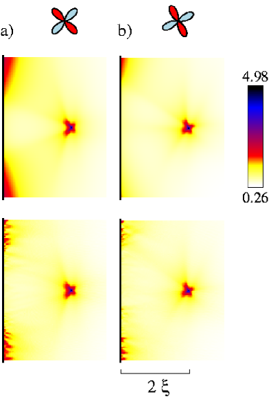
Figure 9: Zero-energy density of states of a $d_{x^{2}-y^{2}}$-wave superconductor in the vicinity of a surface. This corresponds to an opening angle of the wedge of $\alpha=\pi$. A single Abrikosov vortex is located at a distance of $2\xi$ from the boundary. In the top row, the boundary is smooth. In the lower row, the boundary is microscopically rough. a) The nodal direction of the $d$-wave is perpendicular to the boundary, which corresponds to $\gamma=\pi/4$. b) The rotation angle is $\gamma=\pi/6$. Compared to a), the orientation changed by 15 degrees.

A simple model of a microscopically rough surface is given by an arrangement of randomly tilted tiny mirrors along the boundary line. The size of each mirror is taken to be about $\xi/40$, which is of an atomic lengthscale for high-$T_{c}$ superconductors. Each mirror is randomly tilted. We have chosen a Gaussian distribution between $-\pi/4$ and $+\pi/4$ for all the tilt angles, with a tilt angle of $0$ corresponding to a parallel alignment of mirror and boundary line. Additionally, we made the simplification, that the mirrors do not extent into the superconductor. Their only function is to reflect an incoming trajectory according to the mirror orientation, thus producing a kind of random scattering at the boundary. There are some further consequences of the simplification made above. On the one hand, the flow field inside the superconductor is not affected by the boundary roughness and is simply the one of a wedge-shaped boundary geometry with opening angle $\alpha=\pi$. On the other hand, multiple reflections at the boundary and the corresponding effects presented in the previous section are excluded. However, it is important to note, that for any boundary orientation, there exist zero-energy bound states in some regions of the boundary line because of the microscopic roughness. This is in agreement with earlier calculations of the zero-bias conductance peak for a rough surface Fogelstroem .

How is the shadow effect due to a vortex affected by such a microscopically rough surface? The zero-energy local density of states for a boundary line with one specific randomly generated mirror arrangement and an adjacent Abrikosov vortex is shown in Fig. 9. In column a), the nodal line of the $d$-wave is perpendicular to the boundary, which corresponds to a (110) surface or $\gamma=\pi/4$, respectively. Although the appearance of the Andreev bound states along the boundary line changes in a characteristic way because of the microscopic roughness, the suppression of the Andreev bound states in a shadow-like region clearly persists. In b), the orientation between boundary and $d$-wave is changed by $15$ degrees. The suppression of the bound states remains, but it is obviously no more symmetric, neither for the smooth nor the microscopically rough boundary. Since the modulus of the phase gradient around the vortex is symmetric, this asymmetry cannot be explained by a Doppler-shifted energy spectrum, where only local surface currents are taken into account. In fact, generally the whole quasiparticle ”history” along its trajectory is very important and may not be neglected. Only in the case of a homogeneous flow field Fogelstroem , for example far away from the vortex, it becomes sufficient to consider solely the local current.

IV.2 Macroscopic roughness

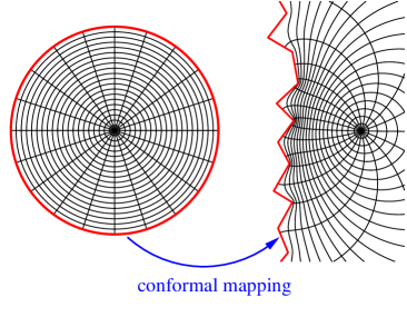
Figure 10: The conformal mapping procedure used to obtain the phase distribution around an Abrikosov vortex in the vicinity of a boundary.

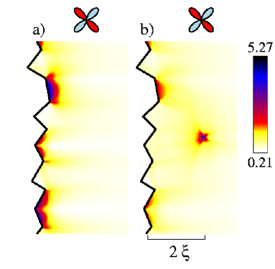
Figure 11: Zero-energy density of states of a $d_{x^{2}-y^{2}}$-wave superconductor with a polygonal boundary geometry, which can be regarded as a boundary line with macroscopic roughness (faceting). a) No vortex is present. b) A single Abrikosov vortex is situated $2\xi$ away from the averaged boundary line.

We now examine the zero-energy local density of states of a $d$-wave superconductor along a macroscopically rough boundary line. As an adequate model, we take a superconductor with a polygonal boundary geometry, consisting of piecewise smooth facets, each of a length of the order of $\xi$. In contrast to the model of a microscopically rough surface presented above, the extension of the polygonal boundary geometry is taken into account completely. For the more simple wedge-shaped boundary in section III, we obtained the phase of the gap function in an analytical way by conformal mapping (cf. section II B). For the more general case of a polygonal boundary, it becomes necessary to calculate the Schwarz-Christoffel mapping Trefethen numerically. We used an implementation by DriscollDriscoll to obtain the correct corresponding phase. This toolbox uses the analytically known solution of the phase distribution for a vortex sitting in the center of a disk and conformally maps this solution onto the vortex close to the polygonal boundary, as illustrated in Fig. 10. For the disk, the lines of constant phase are just radial lines, and the phase gradient corresponds to concentric circles, fulfilling the boundary condition that the phase gradient is parallel to the surface. The toolbox provides the mapping which maps the center of the disk onto the vortex position and the boundary of the disk onto the polygonal boundary. The resulting lines of constant phase and phase gradient after this mapping are shown in Fig. 10, right panel. This means, that within the approximation (9), the currents due to a single Abrikosov vortex are forced to be parallel to each facet of the polygonal boundary. Furthermore, the polygonal boundary allows for multiple reflections of quasiparticle trajectories. Thus, the effects discussed in section III can be found here as well.

In Fig. 11a) and b), the zero-energy local density of states of the $d$-wave superconductor with polygonal boundary structure is shown. The main direction of the boundary is oriented in such a way, that facets parallel to it exhibit maximum Andreev bound states. If we compare the local density of states shown in Fig. 11a), where no vortex is present, to the case with Abrikosov vortex presented in b), many of the effects already discussed above can be found again (cf. for example Fig. 7). The energy spectrum in the corner of a right-angled wedge is, independent of its orientation, the $d$-wave bulk spectrum. Thus, the nearly right-angled parts of the boundary exhibit a very low zero-energy density of states, which is hardly affected by the presence of the vortex. The main effect of the vortex is again a strong suppression of zero-energy bound states in its shadow region. This is because the zero-energy spectral weight is effectively shifted towards higher energies. Bound states at the boundary, which are further away, are reduced more moderately.

V Conclusions

In this work, we investigated the influence of both the boundary geometry and a single pinned Abrikosov vortex on the zero-energy local density of states along the boundary of a $d_{x^{2}-y^{2}}$-wave superconductor. We found that a wedge-shaped boundary can induce a quasiparticle spectrum in the corner of the wedge, which is completely different to that farther away from the corner. The main mechanism for this effect is the multiple reflection of quasiparticle trajectories. In the corner, this can effectively be described as a mixing of bulk trajectories belonging to different angles. Depending on the opening angle of the wedge and the orientation between $d$-wave and boundary geometry, this mixing can either lead to bulk spectra in the corner (and thus to an absence of bound states) or to the presence of induced zero-energy bound states. In Fig. 5a), we have provided a map, showing for which combinations of opening angle and $d$-wave orientation bound states appear. If the wedge is oriented in such a way, that the nodal direction of the $d$-wave is parallel to the bisecting line, the zero-energy density of states in the corner strongly oscillates as a function of the opening angle of the wedge. Although all results presented here have been obtained using a model gap function, a fully selfconsistent calculation is not going to change the results qualitatively. The amplitude of the oscillations mentioned above, for example, should be somewhat reduced, especially for smaller opening angles. But in any case, it should be possible to observe the oscillations at least for larger opening angles.

Another example of an induced quasiparticle spectrum is a wedge with opening angle $\pi/2$: The local density of states in the corner of a right-angled wedge is always given by a $d$-wave bulk spectrum, even if the orientation allows the highest Andreev bound states at both boundary lines. In addition to this geometrically induced prohibition of bound states, we presented the influence of a single pinned Abrikosov vortex on the zero-energy local density of states at the boundary. Bound states at the boundary are locally suppressed, in particular in a shadow-like region close to the vortex. However, this kind of suppression is due to a splitting of the high zero-energy peak of the bound states. Thus it is of a different physical origin. The spectral weight is effectively shifted towards higher energies, because the quasiparticles ”see” a locally varying energy shift along their trajectory, which stems from the locally varying flow field around the vortex. Both effects can be observed independently in our results.

We have studied the influence of two types of surface roughness on the vortex shadow effect: microscopic, random scattering at the surface as well as a more macroscopic faceting of the boundary. In the second case we have taken care to calculate the flow field with the appropriate boundary conditions using the conformal mapping technique. In both cases the vortex shadow effect clearly persists.

- (1) C. R. Hu, Phys. Rev. Lett. 72, 1526 (1994).
- (2) Y. Tanaka and S. Kashiwaya, Phys. Rev. Lett. 74, 3451 (1995).
- (3) L. J. Buchholtz, M. Palumbo, D. Rainer, and J. A. Sauls, J. Low Temp. Phys. 101, 1099 (1995).
- (4) I. Iguchi, W. Wang, M. Yamazaki, Y. Tanaka, and S. Kashiwaya, Phys. Rev. B 62, R6131 (2000).
- (5) J. Lesueur, L. H. Greene, W. L. Feldmann, and A. Inam, Physica C 191, 325 (1992).
- (6) M. Covington, R. Scheuerer, K. Bloom, and L. H. Greene, Appl. Phys. Lett. 68, 1717 (1996).
- (7) S. Graser, C. Iniotakis, T. Dahm, and N. Schopohl, Phys. Rev. Lett. 93, 247001 (2004).
- (8) M. Fogelström, D. Rainer, and J. A. Sauls, Phys. Rev. Lett. 79, 281 (1997).
- (9) M. Covington, M. Aprili, E. Paraoanu, L. H. Greene, F. Xu, J. Zhu, and C. A. Mirkin, Phys. Rev. Lett. 79, 277 (1997).
- (10) M. Aprili, E. Badica, and L. H. Greene, Phys. Rev. Lett. 83, 4630 (1999).
- (11) Y. Dagan and G. Deutscher, Phys. Rev. Lett. 87, 177004 (2001).
- (12) G. Eilenberger, Z. Phys. 214, 195 (1968).
- (13) A. I. Larkin and Yu. N. Ovchinnikov, Zh. Eksp. Teor. Fiz. 55, 2262 (1968) [Sov. Phys. JETP 28, 1200 (1969)].
- (14) N. Schopohl and K. Maki, Phys. Rev. B 52, 490 (1995); N. Schopohl, cond-mat/9804064 (unpublished).
- (15) T. Dahm, S. Graser, C. Iniotakis, and N. Schopohl, Phys. Rev. B 66, 144515 (2002).
- (16) L. J. Buchholtz and D. Rainer, Z. Phys. B 35, 151 (1979).
- (17) A. V. Zaitsev, Zh. Eksp. Teor. Fiz. 86, 1742 (1984) [Sov. Phys. JETP 59, 1015 (1984)].
- (18) A. Shelankov and M. Ozana, Phys. Rev. B 61, 7077 (2000).
- (19) L. Kramer and W. Pesch, Z. Phys. 269, 59 (1974).
- (20) E. V. Thuneberg, M. Fogelström, and J. Kurkijärvi, Physica B 178, 176 (1992).
- (21) T. A. Driscoll and L. N. Trefethen, Schwarz-Christoffel Mapping (Cambridge University Press, 2002).
- (22) T. A. Driscoll, ACM Transactions on Mathematical Software 22(2), 168-186 (1996); Algorithm 756. A more recent version of the Schwarz-Christoffel toolbox for MATLAB is available at T. A. Driscoll‘s website.