Realizing non-Abelian statistics

Abstract

We construct a series of 2+1-dimensional models whose quasiparticles obey non-Abelian statistics. The adiabatic transport of quasiparticles is described by using a correspondence between the braid matrix of the particles and the scattering matrix of 1+1-dimensional field theories. We discuss in depth lattice and continuum models whose braiding is that of $SO(3)$ Chern-Simons gauge theory, including the simplest type of non-Abelian statistics, involving just one type of quasiparticle. The ground-state wave function of an $SO(3)$ model is related to a loop description of the classical two-dimensional Potts model. We discuss the transition from a topological phase to a conventionally-ordered phase, showing in some cases there is a quantum critical point.

I Introduction

Understanding phases with topological order has become an important theme in condensed-matter physics. Well-understood examples of topological fluids include the fractional quantum Hall states which arise for electrons in two dimensions moving in large magnetic fields. The existence of quasiparticles or quasiholes with fractional statistics is a central and striking prediction of the theory of the fractional quantum Hall effect and follows directly from the nature of the electronic correlations in this quantum fluidlaughlin ; arovas . In spite of its profound conceptual importance, only this week has there been a report of experimental confirmation of this startling predictiongoldman .

Non-Abelian fractional statistics are a fascinating property of some fractional quantum Hall states moore92 . Here, the wave function depends not only on which particles are braided, but on the order in which they are braided: the states carry a non-Abelian (matrix) representation of the braid group. One of the motivations for the current consideration of non-Abelian phases is the realization that a physical system in a non-Abelian topological phase behaves effectively as a universal quantum computerkitaev ; freedman01 ; freedman03 .

The topological quantum fluids arising in the fractional quantum Hall effect have an effective hydrodynamical description in terms of Chern-Simons gauge theoriesfqh-cs ; wen-zee ; wen-review . Pure Chern-Simons is a topological field theory, meaning that its correlators are independent of the position of the operators and depend only on topological invariantswitten89 . It has a vanishing Hamiltonian; the only non-trivial properties arise from the braiding of its Wilson and its Polyakov loops. In this paper we are mainly interested in theories whose ground state is topological, but whose gapped excitations have non-Abelian statistics.

Fractional quantum Hall fluids do not have time-reversal symmetry, but topological order occurs in models with unbroken time-reversal invariance as well. These “spin-liquid” phases were originally speculated to be responsible for the unusual behavior of the “normal state” of high temperature superconductorspwa ; krs although, in spite of much effort both theoretical and experimental, there is yet no solid evidence for any spin-liquid state. Nevertheless, as a consequence of much (theoretical) effort, we know that topological order occurs in the ground states in certain gapped systems with time-reversal invariance and reasonably-local interactionskitaev , for example in quantum dimer models on non-bipartite latticesRK ; moessner-sondhi . Morally, these topological phases are equivalent (in the sense of asymptotic low energy theories) to deconfined phases of an effective gauge theory. The excitations of these time-reversal invariant phases do exhibit electron fractionalizationkivelson87 ; read-chak ; read-sachdev ; senthil-fisher , but the statistics is Abelian.

Non-Abelian topological phases are even harder to come by. Such phases with broken time-reversal symmetry do occur in the fermionic Pfaffian (a.k.a. Moore-Read) wave function moore92 for the $\nu=5/2$ fractional quantum Hall effect, and in the $\nu=1$ bosonic Pfaffian stateread-rezayi ; FNS ; ardonne99 . The former occurs in models of $p$-wave superconductors as well ivanov . Field theories with such non-abelian statistics also have been found alford ; Lo ; bais . In a number of these cases, the long-distance physics can be described by a Chern-Simons gauge theory, which breaks time-reversal symmetry. Non-abelian topological phases, however, occur in time-reversal-invariant systems as wellfreedman01 ; freedman03 . The resulting effective Chern-Simons theory is doubled to restore the time-reversal symmetry. To give the theory a gap while keeping the topological theory as its ground state, one can include the electric-field part of the Maxwell term $\int d^{2}x\;\vec{E}\cdot\vec{E}$ in the Hamiltonian witten92 ; grignani ; ardonne . Hence in these topological phases, the ground-state wave function is a superposition of configurations of Wilson loops in two-dimensional space, while the world-lines of the excitations correspond to Polyakov loops in the 2+1-dimensional field theory freedman03 . For example, the lattice models discussed in detail in Refs. freedman-nayak-shtengel-03, ; freedman04, have a continuum description in terms of doubled $SU(2)_{k}$ Chern-Simons gauge theory. The resulting configuration space is naturally associated with the Temperley-Lieb algebraTL .

A natural description of the configuration space of models in a topological phase is in terms of loops kitaev ; freedman01 ; freedman03 ; freedman-nayak-shtengel-03 ; freedman04 . This holds in both Abelian and non-Abelian cases. Precisely, each basis state in the Hilbert space of the quantum theory is a loop configuration in two dimensions. Quantum dimer models and their generalizations ardonne ; chamon can also be viewed as quantum loop gases.

In this paper we reexamine the problem of non-Abelian topological phases by starting with the statistics we wish to have, and working backward to construct a model which exhibits them. We thus first give an algebraic way of characterizing the braiding in both $SU(2)_{k}$ and $SO(3)_{k}$ Chern-Simons theories. We show that such a braid matrix of a 2+1-dimensional theory is a limit of the $S$-matrix of an associated relativistic 1+1 dimensional model, and give an intuitive argument as to why this is so. We then show how to explicitly construct quantum two-dimensional models with these braid relations by utilizing the structure of the factorizable $S$-matrices of integrable 1+1-dimensional models.

Specifically, we embed the 1+1-dimensional model in two-dimensional Euclidean space, and find a Rokhsar-Kivelson-type quantum HamiltonianRK acting on this two-dimensional space whose ground state has the properties expected of a model with non-Abelian statistics. In both cases we discuss in detail, the Hilbert space is that of a loop gas: in the $SU(2)_{k}$ case, the loops are self-avoiding and mutually-avoidingfreedman04 , while in the $SO(3)_{k}$ case, the loops intersect. The latter are thus more akin to nets than loopslevin03 . Both these loop gases are associated with well-known two-dimensional classical statistical mechanical models: in the $SU(2)_{k}$ case, this is the known as the $O(n)$ lattice model with $n=2\cos(\pi/(k+2))$, while in the $SO(3)_{k}$ case, this is the $Q$-state Potts model with $Q=4\cos^{2}(\pi/(k+2))$. The loop expansion of the former is well knownnienhuis , but the one we utilize for the Potts model does not seem to have been discussed before.

Having an explicit lattice construction of the states enables us to construct (reasonably) local quantum lattice models with these ground state wave functions. By studying the statistical properties of the absolute value squared of these wave functions, we can investigate the correlations described by these quantum states, and determine if they describe quantum critical points or massive (topological) phases. Both here and in the $SU(2)$ casefreedman-nayak-shtengel-03 , the result depends on the level $k$.

The paper is organized as follows. In Section II we describe the algebraic approach to non-Abelian statistics in both the $SU(2)_{k}$ case and $SO(3)_{k}$ cases. In Section III we discuss quantum loop gases and their relation to the $S$ matrix of 1+1-dimensional integrable field theories. In Section IV we give an explicit construction of these $S$-matrices for $SO(3)$ and $SU(2)$ braiding. In Section V we discuss the corresponding 1+1-dimensional field theories. In Section VI we discuss lattice models whose ground states are precisely the loop wave functions, both $SU(2)_{k}$ and $SO(3)_{k}$, with the desired braiding properties. We give a set of specific criteria that 2+1-dimensional quantum Hamiltonian ought to satisfy and give an explicit construction. In Section VII we discuss under what circumstances these wave functions are topological and when do they describe quantum critical systems. In Appendix A we give a summary of the Landau-Ginzburg description of the 1+1-dimensional theories whose $S$ matrix we use.

II Braids and Algebras

Particle statistics, of course, are the effect on the wave function when particles are adiabatically transported around each other a large distance away. This picture follows from the familiar concept of adiabatic particle transport, developed in detail in the context of the Laughlin states of the fractional quantum Hall effect where it follows from the Berry phase accumulated during an adiabatic evolution of the state with two quasiparticlesarovas .

Adiabatic particle transport can be represented pictorially by drawing the world lines of the particles, which are the paths they trace out in space-time. Since the particles stay far apart, we need only study paths which do not cross. (Non-trivial braid statistics always require the assumption that particles have a hard-core short distance repulsion). The world lines of the particles therefore braid around each other. Formally, the set of all possible braidings is a group, acting on the space of states of the system. Different types of statistics correspond to different representations of the braid group. In this paper we consider two spatial dimensions, where both Abelian and non-Abelian statistics are possible. A system whose quasiparticles are associated with a non-Abelian representation of the braid group has a degenerate set of states of quasiparticles at fixed positions ${x_{1}},{x_{2}},\ldots,{x_{N}}$. Call this space of states $V(N)$. The states in $V(N)$ are locally indistinguishable but differ topologically. When a quasiparticle is taken around another, states in this degenerate subspace are rotated into each other. Since this is quantum mechanics, it can take a state to a linear combination of other states: adiabatic particle transport can entangle the states.

Although we will not require its use, it is useful to note that non-Abelian statistics can be implemented in a local field theory by assigning to each quasiparticle a charge and a flux under a non-Abelian gauge group. Within this picture, a quasiparticle carries a representation $V$ (i.e. a ‘charge’) of the gauge group $G$ and a flux $g\in G$. When quasiparticle $1$ is taken around quasiparticle 2, its internal state ${\psi_{1}}\in V_{1}$ is rotated to ${g_{2}}\psi_{1}$ by the action of the flux ${g_{2}}\in G$ which is associated with quasiparticle 2. It is worth keeping in mind that this picture is not gauge invariant, and there is, in fact, no local degree of freedom associated with each quasiparticle (since a gauge transformation can change $\psi\in V$ into any other $\psi^{\prime}\in V$ and can change the flux $g$ into any other element of its conjugacy class $hgh^{-1}$).

Studying the statistics of a 2+1-dimensional system can effectively be reduced to a two-dimensional problem. We project the world lines onto the plane (ignoring boundary conditions), and call them strands. When there are $N$ particles, we have $N$ strands. A braiding in 2+1 dimensions results in the crossing of two strands in the two-dimensional picture. In this projection, there are overcrossings and undercrossings. As long as we are only interested in the statistics of the particles, the other details of the projection are not particularly important: we can move the strands around at will as long as we do not remove crossings or create new ones.

It is useful to think of this collection of strands in the plane in a 1+1-dimensional fashion. The degenerate states of the 2+1-dimensional system correspond to a set of degenerate multi-particle states in a one-dimensional quantum system. In this 1+1-dimensional quantum system, each strand is the world line of a real local degree of freedom. Heuristically, this is the “gauge-fixed” version of the model. Consider a configuration at $t=-\infty$ (i.e. before any of the particles have been braided) where all the particles are very far from each other (i.e. all at spatial infinity). We can thus consider these particles to all be on a circle. This circle is our one-dimensional space. We can construct the full configuration by a sequence of adiabatic braidings as the particles move inward. Since we are free to move around the strands as long as we do not add or remove crossings, we can then take all the particles at $t=\infty$ to lie on a circle as well. Thus we can project all the original 2+1-dimensional world-lines onto a two-dimensional annulus. We can then view the angular direction of the annulus as one-dimensional space, and the radial direction as (Euclidean) time. Thus, each configuration in the plane can be regarded as an adiabatic evolution in an equivalent 1+1-dimensional Euclidean field theory in which each strand (or particle) belongs to a given Hilbert space associated with the species.

To make this more precise, let us consider the $N$-particle space of states $V(N)$ on which the braid group acts. For now we let this space be the tensor product of $N$ copies of the single-particle space of states: $V(N)=V^{\otimes N}\equiv V_{1}\otimes V_{2}\otimes\dots\otimes V_{N}$. (Later, we will see that the actual space of states is a subspace of $V^{\otimes N}$.) In the 1+1 dimensional picture, we can think of $V^{\otimes N}$ as the space of particles on a circle. The elements of the braid group corresponding to overcrossings and undercrossings are denoted $B_{i}$ and $B_{i}^{-1}$ and are displayed in Fig. 1.

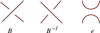
Figure 1: braid, reverse braid, and Temperley-Lieb generator

The subscript $i$ means that $B_{i}$ is describing the crossing between the $i$th and the $(i+1)$th particles, and so acts non-trivially on the space $V_{i}\otimes V_{i+1}$, and with the identity on the other spaces $V_{j}$, with $j\neq i,i+1$. For example, the braids in Fig. 2

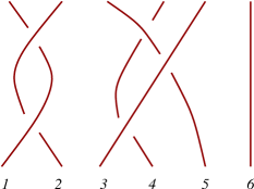
Figure 2: A typical braiding involving six particles

are described algebraically as $=B_{3}^{-1}B_{4}B_{3}B_{1}B_{1}$. The braid-group generators $B_{i}$ must satisfy the relations

$$B_{i}B_{i+1}B_{i} = B_{i+1}B_{i}B_{i+1},$$

$$B_{i}B_{j} = B_{j}B_{i}\qquad\qquad|i-j|\geq 2.$$ (1)

These relate configurations which are topologically identical, as can easily be seen from Fig. 3.

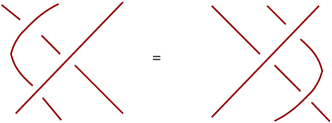
Figure 3: Consistency relation for braiding

If the matrices $B_{i}$ are diagonal, then the statistics are Abelian. For bosons the $B_{i}$ matrices are all the identity; for anyons their entries are phases. In this paper we are interested in non-Abelian representations of the braid group, so that particles obey non-Abelian statistics: the wave function changes form depending on the order in which the particles are braided. One can give explicit matrix representations of the braid group. However, it is usually much convenient to study the algebra of the matrices involved. In the cases of interest here, the statistics of the particles can be obtained directly from the algebraic relations the matrices obey, without need for their explicit representation.

II.1 The $SU(2)$ theory

A famous one-parameter set of non-Abelian representations of the braid group arises from utilizing the Temperley-Lieb algebra TL . These representations give rise to the Jones polynomial in knot theory Jones ; Kauffman ; ADW , and correspond to the braiding of Wilson and Polyakov loops in $SU(2)$ Chern-Simons theory.

The Temperley-Lieb algebra originally arose as a way of relating the Potts models to the six-vertex model. The transfer matrices of these two models (and a number of other models) can be written in terms of different representations of this algebra. This means that any properties of the model which can be computed from purely algebraic considerations will be the same for any such model. A generator of the Temperley-Lieb algebra $e_{i}$ acts non-trivially on the $i$th and $(i+1)$th particles; a useful pictorial representation is given in Fig. 1. The algebra is TL

$$e_{i}^{2} = de_{i},$$

$$e_{i}\,e_{i\pm 1}\,e_{i} = e_{i},$$

$$e_{i}\,e_{j} = e_{j}\,e_{i}\quad(|j-i|\geq 2).$$ (2)

where $d$ is a parameter. These algebraic relations are drawn in Fig. 4.

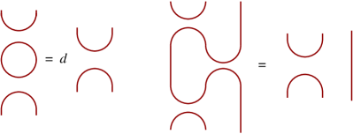
Figure 4: The Temperley-Lieb algebra

From the picture, one can see that $d$ can be thought of as the weight of a closed loop.

Representations of the braid group can be found from representations of the Temperley-Lieb algebra by letting

$$B_{i}=I-qe_{i},$$ (3)

where $I$ is the identity. This is illustrated in Fig. 5.

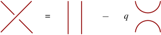
Figure 5: The braid in terms of the Temperley-Lieb generator

The $B_{i}$ defined in this fashion obey the braid-group relation (1) when

$$d=q+q^{-1}.$$

It is also easy to check that

$$B_{i}^{-1}=I-q^{-1}e_{i}.$$

Note that in writing the braid group in this fashion, we have resolved the crossings $B$ and $B^{-1}$ in terms of strands which no longer intersect.

These braid relations are those of Wilson loops in $SU(2)_{k}$ Chern-Simons theory when witten89

$$d=2\cos\left(\frac{\pi}{k+2}\right)$$

or equivalently $q=e^{i\pi/(k+2)}$. The integer $k$ is the coefficient of the Chern-Simons term in the gauge theory, and is known as the level. It must be an integer to ensure gauge invariance of the Chern-Simons gauge theory deserjackiw .

The configuration space of Wilson loops on the plane is a very large space and arbitrary superpositions of these states do not obviously describe a topological ground state. It turns out that in order to enforce the condition that states be purely topological, these ground states must satisfy additional properties which can be enforced by means of a suitable projection operator. This is known as the Jones-Wenzl projector, which acts on $k+1$ strands without crossings. For details on its application in this context, see Refs. freedman01, ; freedman03, . We will give an algebraic description of this below. By construction, states obtained by means of this projector are topological and do not support local low energy degrees of freedom. Conversely, unprojected states can describe low energy, even massless, degrees of freedom, and are unphysical states in a topological gauge theory such as Chern-Simons. However, unprojected states may describe degrees of freedom associated with quantum critical points.

II.2 The $SO(3)$ theory

Here we discuss another one-parameter set of non-Abelian representations of the braid group. These describe the braiding in $SO(3)$ Chern-Simons theory, instead of $SU(2)$. The algebras are of course the same; the key distinction is that Wilson and Polyakov loops in $SO(3)$ Chern-Simons occur in only integer-spin representations. The corresponding representation of the braid group is given in terms of the $SO(3)$ Birman-Murakami-Wenzl (BMW) algebra BMW , defined below. This algebra has two non-trivial generators $X_{j}$ and $E_{j}$ acting on adjacent strands.

The $SO(3)$ braid relations can be found by “fusing” together two strands obeying the Temperley-Lieb algebra: the $SO(3)$ BMW generators $X_{j}$ and $E_{j}$ can be written in terms of the Temperley-Lieb generators $e_{i}$. Heuristically, the idea is to exploit the fact that a spin-1 representation of $SO(3)$ can be found from the tensor product of two spin-$1/2$ representations of $SU(2)$. This statement is still true in the “quantum-group” algebra $U_{q}(sl_{2})$, which is a one-parameter deformation of the ordinary Lie algebra $sl_{2}$. One can define an action of $U_{q}(sl_{2})$ on the space of states $V^{\otimes N}$ which commutes with the $e_{i}$; see Ref. slingerland, for an extensive discussion of quantum groups in the context of non-Abelian statistics ($q$ there is $q^{2}$ here). In particular, to relate the two algebras, first note that $e_{i}/d$ is a projector. In $U_{q}(sl_{2})$ language, this projects onto the trivial spin-0 representation. The projector onto the spin-1 representation is therefore

$$P_{i}=I-\frac{1}{d}\,e_{i},$$ (4)

so that $P_{i}e_{i}=0$. The single-particle space of states $W_{j}$ in the $so(3)$ BMW algebra is comprised of two “fused” Temperley-Lieb strands, projected onto the spin-1 representation. In an equation, $W_{j}=P_{2j-1}[V_{2j-1}\otimes V_{2j}]$. Pictorially, just think of each strand in the $so(3)$ theory as the left-hand-side of Fig. 6.

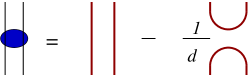
Figure 6: Projecting onto the spin-1 representation

With this identification, the $so(3)$ BMW algebra follows from the Temperley-Lieb algebra. Since lines never cross in the latter, they cannot cross in the former either. When two of the fused strands come near each other, there are now three possibilities for what happens, which we display in Fig. 7.

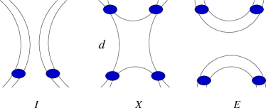
Figure 7: The generators of the $SO(3)$ BMW algebra

From the pictures, we read off that

$$E_{j} = {P}_{2j-1}\,{P}_{2j+1}\,e_{2j}\,e_{2j-1}\,e_{2j+1}\,e_{2j}\,{P}_{2j-1}\,{P}_{2j+1},$$ (5)

$$X_{j} = d\ {P}_{2j-1}\,{P}_{2j+1}\,e_{2j}\,{P}_{2j-1}\,{P}_{2j+1}.$$ (7)

These generators act on the two-particle states in $W_{j}\otimes W_{j+1}$. It is straightforward to verify using (2) that they obey the $o(3)$ BMW algebra. We have

$$(E_{i})^{2} = (Q-1)E_{i},$$

$$(X_{i})^{2} = (Q-2)X_{i}+E_{i}.$$

$$E_{i}X_{i}=X_{i}E_{i} = (Q-1)E_{i}.$$ (8)

where the parameter $Q\equiv d^{2}$.

Relations involving generators on adjacent sites (e.g. $E_{i}E_{i+1}E_{i}=E_{i}$) are straightforward to work out using the Temperley-Lieb algebra; they can be found for example in Ref. fendleyread, . Most become fairly obvious after drawing the appropriate picture. The relations involving only the $E_{i}$ are those of the Temperley-Lieb algebra (2), but with $d$ replaced here by $Q-1$, so that closed isolated loops of “spin-1” particles get a weight $Q-1=d^{2}-1=1+q^{2}+q^{-2}$. This factor of $d^{2}-1$ is obvious from the pictures; the $d^{2}$ comes from the $d$ from each loop, and $1$ must be subtracted because of the projection onto spin-1 states (projecting out the singlet).

The reason we have done all this work is to give us another representation of the braid group. Namely, defining

$$B^{SO(3)}_{j} = q^{2}{\cal I}-X_{j}+q^{-2}E_{j},$$ (9)

it is straightforward to check using the $so(3)$ BMW relations that the $B_{j}$ satisfy the braid-group relations (1). ${\cal I}$ is the identity on the projected Hilbert space $W^{\otimes N}$; on $V^{\otimes N}$, we have ${\cal I}=P_{2j-1}P_{2j+1}$ (see Fig.7). One can also check that

$$(B^{SO(3)}_{j})^{-1}=q^{-2}{\cal I}-X_{j}+q^{2}E_{j}.$$

Particles with braiding given by $B^{SO(3)}_{j}$ arise from $SO(3)$ Chern-Simons theory. This follows from our construction: we basically have restricted the particles to be associated with integer-spin representations of $U_{q}(sl_{2})$; this is precisely what one does to go from $SU(2)$ to $SO(3)$.

II.3 The Jones-Wenzl projector

The Jones-Wenzl projector is simply expressed in terms the projector ${\cal P}^{(s)}$ onto the representation of spin $s$ of $U_{q}(sl_{2})$: for a given $k$ it is simply ${\cal P}^{([k+1]/2)}_{j}=0$ for all $j$. This projector involves $k+1$ strands, so this amounts to being able to replace the identity acting on $k+1$ strands with a linear combination of other Temperley-Lieb or BMW elements. The necessity of this projection is also apparent from the representation theory of $U_{q}(sl_{2})$: when $q^{k+2}=-1$, the spin-$(k+1)/2$ representation is reducible but is indecomposable (it cannot be written as a direct sum of irreducible representations). Performing the projection avoids all sorts of complications such as zero-norm states.

We have already seen one example of such a projector. The projector $P_{i}=I-e_{i}/d$ is the projector onto the spin-1 representation of the quantum-group algebra, so ${\cal P}^{(1)}_{j}=P_{j}$. When $k=1\ (d=1)$, the Jones-Wenzl projector is simply $P_{j}$: any spin-1 combination of strands is projected out. Therefore the $SO(3)$ theory at $k=1$ is trivial.

A case of great interest is $SO(3)_{3}$, the “Lee-Yang” model. This is the simplest model of non-abelian statistics, because there is only one type of non-trivial braiding. The naming arises because the braiding relation for the particle in this model is the same as the fusion rule associated with the Lee-Yang conformal field theorycardy . We have for any $k$ in both the $SU(2)$ and $SO(3)$ models

$${\cal P}^{(2)}_{j}=P_{2j-1}P_{2j+1}-\frac{1}{d^{2}-2}X_{j}+\frac{1}{(d^{2}-2)(d^{2}-1)}E_{j}$$ (10)

When $k=3$, the Jones-Wenzl projector sets ${\cal P}^{(2)}=0$. In the $SU(2)_{3}$ theory, this is a relation involving four strands, while in the $SO(3)_{3}$ theory, this relates two of the fused strands. This means that in $SO(3)_{3}$, imposing the Jones-Wenzl projector allows us to replace any appearance of a generator $X_{j}$ in favor of ${\cal I}$ and the $E_{j}$: we have

$$X_{j}=(Q-2)({\cal I}+E_{j})\qquad\qquad\hbox{for }SO(3)_{3}.$$

Plugging this back into the braid relation (9) and remembering that $Q-2=q^{2}+q^{-2}$ gives

$$B^{SO(3)_{3}}_{j} = -q^{2}{\cal I}-q^{-2}E_{j}.$$ (11)

Note that for this value $k=3$ (and this value alone), the generators $E_{j}$ obey the same Temperley-Lieb algebra as the $e_{i}$, because $d=2\cos(\pi/5)=d^{2}-1$. Moreover, $q^{5}=-1$ here, so the braid generator (11) is equivalent to that in (3). We thus are led to an intriguing result: the $O(3)_{3}$ theory is almost identical to that of $SU(2)_{3}$. There is one important difference: in $SO(3)_{3}$, we have already imposed the Jones-Wenzl projector, while in $SU(2)_{3}$ this still needs to be imposed. Thus (locally) $SO(3)_{3}$ with the Jones-Wenzl projection imposed is equivalent to $SU(2)_{3}$ without it imposed.

III Quantum loop gases and the $S$ matrix

In the preceding section we discussed some of the marvelous properties of particles with non-Abelian statistics. Now we discuss how to associate the $S$ matrix of a relativistic 1+1-dimensional field theory to the type of braiding discussed above. We argue that knowing the $S$ matrix in this 1+1-dimensional theory allows us to find a quantum loop gas in two space dimensions where the quasiparticles should have these braid relations.

A natural place to look for models with non-Abelian statistics is in quantum loop gases. The reason is that if one projects the world lines onto the (spatial) plane, one obtains loops: strands cannot end. It is also natural from the point-of-view of field theory: in pure Chern-Simons theory the only gauge-invariant degrees of freedom are loops. In a 2+1-dimensional picture, this means it is a good idea to look for a system where the low-energy degrees of freedom are loops in the plane, a quantum loop gas. In a number of cases it has been argued that quantum loop gases turn into gauge theories with Chern-Simons theories in the continuum freedman01 ; freedman03 ; levin03 ; ardonne . The excitations can be non-Abelian in a topological phase, where the ground state contains a superposition of Wilson loops (loops in the spatial plane). The excited states are Polyakov loops, loops which extend in the time direction. The quasiparticles have non-Abelian statistics when the gauge group is non-Abelian with level $k>1$, Ref. witten89, .

To understand these loop gases, it is best to first focus on the properties of the ground state. The types of ground states we are interested in are liquid states, where all local order parameters have vanishing expectation values. Such a ground state is a superposition of different loop configurations. The basis states $|s\rangle$ of the Hilbert space can all be described by some configuration of loops in two dimensions. In these models, the wave function $\Psi$ of this ground state can be written in the form

$$\langle s|\Psi\rangle=\frac{e^{-{\cal S}(s)}}{Z}$$ (12)

where ${\cal S}(s)$ turns out to be the action of the classical two-dimensional loop model for the configuration corresponding to $s$. $Z$ is the usual two-dimensional partition function with weight $|\langle s|\Psi\rangle|^{2}$, which is the functional integral over all configurations $s$ with weight $e^{-{\cal S}(s)-{\cal S}^{*}(s)}$. However, just because the loops can be non-local does not mean the action needs to have long-range interactions. Recall, for example, that one can describe all the configurations in the classical two-dimensional Ising model in terms of closed loops of arbitrary length, the domain walls. Nevertheless, the interactions are still local.

Since we are identifying the loops with the quasiparticle world lines, we need to find a quantum loop gas whose ground-state wave function satisfies the appropriate braiding properties. To make this notion precise, let us examine the classical loop gas (i.e. the one with action ${\cal S}(s)$) corresponding to the ground state. Now view this two-dimensional loop gas as a 1+1-dimensional quantum system. The loops then can be thought of as world lines of particles in this 1+1-dimensional system. Their wave function is then a vector in the space $V^{\otimes N}$, just like before. The braid generators act in the same way as well.

To summarize the arguments so far: we project the world lines of the particles in 2+1 dimensions down onto the plane, so that they form loops. A two-dimensional quantum system possessing such particles is a loop gas, where the degrees of freedom are loops in the plane. The ground-state wave function of the quantum system is the expressed in terms of the action ${\cal S}(s)$ of the corresponding classical two-dimensional loop gas. Finally, we then identify these loops as the world lines of particles in the corresponding 1+1-dimensional problem. The upshot is that by restricting ourself to considering the ground state, we have reduced a 2+1-dimensional problem to a 1+1-dimensional one. Theories for which this construction holds are inherently holographic in that the degrees of freedom can be naturally projected to a boundary.

In the 1+1-dimensional theory, when two particle world lines cross, the $S$ matrix plays the role of the braid matrix. In other words, it describes what happens to the wave function when the paths of two particles cross. Consider the wave function describing two particles of momentum and position $p_{i},x_{i}$ and $p_{i+1},x_{i+1}$ respectively. The $S$ matrix is a matching condition on the wave functions for $x_{i}\ll x_{i+1}$ and $x_{i}\gg x_{i+1}$. As before, the wave function is a vector in $V^{\otimes N}$. The two-particle $S$ matrix for scattering particle $i$ from particle $i+1$ acts non-trivially in $V_{i}\otimes V_{i+1}$:

$$\psi_{V_{i}\otimes V_{i+1}}({x_{i}\gg x_{i+1}})=S_{i}(p_{i},p_{i+1})\psi_{V_{i}\otimes V_{i+1}}(x_{i}\ll x_{i+1}).$$

Our theories are rotationally invariant in two-dimensional space, so the corresponding 1+1-dimensional theory is Lorentz invariant. This means that the $S$ matrix depends only on the relative rapidity $\theta$: defining $p_{i}=m\sinh\theta_{i}$ and $p_{i+1}=m\sinh\theta_{i+1}$, we have $\theta\equiv\theta_{1}-\theta_{2}$. We note that the $S$ matrix here should not be confused with what is usually called the modular $S$ matrix, which governs the braidings in Chern-Simons theory and in conformal field theory.

This correspondence between the braid group and the $S$ matrix has long been known, in the context of knot theory ADW . Representations of the braid group (and the resulting knot invariants) can be found by taking a special limit of solutions of the Yang-Baxter equation ADW . In physics, the Yang-Baxter equation arises in integrable lattice models and field theories. In integrable lattice models, the Boltzmann weights must satisfy Yang-Baxter; in the former, the $S$ matrices of the particles do! Note, moreover, that the braid matrices and the $S$ matrices are acting in the same space $V^{\otimes N}$. So our arguments indicate that the braid matrices of the 2+1-dimensional theory are a limit of the $S$ matrices of the corresponding 1+1-dimensional theory.

It is not difficult to find in which limit this holds. The Yang-Baxter equation for the $S$ matrix arises from requiring that the three-body $S$ matrix factorizes into a product of two-body ones. Since there are two different ways of factorizing, for consistency one must have

$$S_{i}(\theta_{1}-\theta_{2})S_{i+1}(\theta_{1}-\theta_{3})S_{i}(\theta_{2}-\theta_{3})\qquad$$

$$=S_{i+1}(\theta_{2}-\theta_{3})S_{i}(\theta_{1}-\theta_{3})S_{i+1}(\theta_{1}-\theta_{2}).$$ (13)

The connection to the braid group is now obvious: $S(0)$ and $S(\infty)$ obey the braid group relation (1). In most known cases (and in the cases of interest here) $S(0)\propto I$, and $S(-\theta)S(\theta)=I$. Thus we have

$$B = \lim_{\theta\to\infty}\widetilde{S}(\theta)$$

$$B^{-1} = \lim_{\theta\to\infty}\widetilde{S}(-\theta)$$ (14)

The matrix $\widetilde{S}=e^{i\delta(\theta)}e^{i\theta A}Se^{i\theta B}$, where $\delta(\theta)$ is a function of the rapidity $\theta$, and $A$ and $B$ are diagonal $\theta$-independent matrices. These factors arise in general to ensure that $S$ has the correct properties under crossing symmetry and unitarity. Obviously, we need to remove the oscillating factors as $\theta\to\infty$ to have a well defined limit. Both $S(\theta)$ and the modified matrix $\widetilde{S}(\theta)$ satisfy the Yang-Baxter equation (13).

The limit $\theta\to\infty$ in Eq. (14) also makes sense at an intuitive level. In order for the $S$ matrix to be that of a loop gas, one should be in a limit where the mass $m$ of the particles is small: otherwise, the loops would be high in energy and not dominate the partition function. When the particle mass is small, one can create particles of any rapidity $\theta_{i}$, and so the rapidity difference $\theta=\theta_{i}-\theta_{i+1}$ will typically be large.

To conclude this section, we note that there are two important additional steps to take in constructing a quantum loop gas having quasiparticles with non-Abelian statistics. The first is to find a Hamiltonian which has the ground-state wave function of Eq. (12). This can usually be done by a trick utilized by Rokhsar and Kivelson RK . This trick is useful for any field theory with an explicit real action arovas91 ; ardonne . For lattice models, there can be complications, because one cannot always construct a Hamiltonian which is ergodic in the Hilbert space. Nevertheless, in many cases of interest this procedure has been successful.

The second additional step is to make sure that the excited states have braid relations which are those of the loops in the ground state. One way of doing this is to have a Hamiltonian so that the excited states are defects in the configuration space of loops. That is, a particle and an antiparticle over the ground state are connected by a strand. Thus when they are moved around each other, the non-locality due to the strand results in the braid relations described above. As is well known, this construction works in the Abelian case.

IV The braid matrices

In this section we give explicit expressions for the $S$ matrices and braid matrices associated with the Temperley-Lieb and BMW algebras described in section II. This will enable us in the next section to identify the two-dimensional classical field theories associated with these 1+1-dimensional quantum theories, so that we can construct quantum loop gases with the desired braiding.

In the $SU(2)$ case, the correspondence given in Eq. (14) means that we need to look for an $S$ matrix which at infinite rapidities is of the form of Eq.(3). Such an $S$ matrix has been known for quite some timesu2-S-matrix . It is straightforward to check that

$$\widetilde{S}_{i}(\theta)=I-\frac{e^{\lambda\theta}-e^{-\lambda\theta}}{q^{-1}e^{\lambda\theta}-qe^{-\lambda\theta}}\,e_{i}$$ (15)

obeys the Yang-Baxter equation (13) for any value of the parameter $\lambda$, as long as $e_{i}$ satisfies the Temperley-Lieb algebra, Eq.(2).

A number of related models have $S$ matrices which can be written in the form of Eq.(15). The most famous is the sine-Gordon model. There are two different particles, the soliton (labeled $+$) and antisoliton (labeled $-$), forming the spin-1/2 representation of the $U_{q}(sl_{2})$ symmetry of the model. The single-particle space of states $V_{i}$ is two-dimensional, so that $e_{i}$ (which acts on $V_{i}\otimes V_{i+1}$) is a four-by-four matrix in this representation of the Temperley-Lieb algebra. Labeling the rows and columns in the order $++$, $+-$, $-+$, $--$ gives

$$e^{6v}_{i}=\begin{pmatrix}0&0&0&0\cr 0&q&1&0\cr 0&1&q^{-1}&0\cr 0&0&0&0\end{pmatrix}$$ (16)

We have labeled this with a $6v$ because the the Boltzmann weights of the six-vertex model can also be expressed in terms of these $e_{i}$.

This particular representation $e^{6v}$ of the Temperley-Lieb algebra, however, does not result in the braid matrices of the 2+1-dimensional theory, as it does not respect the Jones-Wenzl projector. Namely, consider $k+2$ strands in a row, i.e. the space $V_{1}\otimes V_{2}\otimes\dots\otimes V_{k+2}$. Any $k+1$ strands in a row must obey the Jones-Wenzl projector: we must restrict the space of states so that ${\cal P}_{1}^{([k+1]/2)}={\cal P}_{2}^{([k+1]/2)}=0$ (the former acts non-trivially on the first $k+1$ strands, the latter on the strands $2\dots k+2$). Now braid the $k+2$th particle with the $k+1$st; the resulting configuration need no longer satisfy ${\cal P}^{([k+1]/2)}_{1}=0$. For example, consider three strands in the $k=1$ case, where configuration $(-+-)$ in $V_{1}\otimes V_{2}\otimes V_{3}$ is part of the projected Hilbert space. If we braid the last two particles, the off-diagonal terms in $e^{6v}$ result in a non-zero amplitude for the final state $(--+)$. The latter state is projected out of the Hilbert space, since two $S_{z}=-1/2$ states in a row are necessarily in a spin-1 representation. Thus the braiding does not commute with the projection: imposing the Jones-Wenzl projector violates unitarity. Obviously, we can’t have this, so the only alternative is to conclude that $e^{6v}_{i}$ from Eq. (16) cannot be used to build a braid matrix.

Luckily, this issue is well-understood from a number of points of view. When $k$ is an integer, there is another representation of the Temperley-Lieb algebra which preserves the projection. In the language of two-dimensional classical statistical mechanical lattice models, this representation is called the restricted solid-on-solid (RSOS) representation ABF ; Pasquier . In the $S$ matrix language, this representation describes the scattering of kinks in potential with $k+1$ degenerate minima, as we discuss in Appendix A. In the quantum-group picture, the RSOS representation is obtained by “truncating” the states, so that all are in irreducible and indecomposable representations of $U_{q}(sl_{2})$.

The presence of the Jones-Wenzl projector means that we do not need to define the braid matrix on the full tensor product $V^{\otimes N}$, but only on the restriction/truncation/projection of the space $V^{\otimes N}$ to the states obeying ${\cal P}_{j}^{([k+1]/2)}V^{\otimes N}=0$ for all $j$. This restricted Hilbert space is our true space of states $V(N)$. The states in $V(N)$ are conveniently labeled in terms of a series of variables we call “dual spins”. (These variables are often called heights; we avoid this here to avoid confusion with the heights we discuss in the next section.) The dual spins take on integer values ranging from $1\dots k+1$, and live between the strands. Each strand is labeled by the two dual spins to the left and right of it, which must differ by $\pm 1$. The key effect of the restriction is the fact that dual spins only range from $1$ to $k+1$. This is a consequence of not allowing $k+1$ consecutive strands to have spin $(k+1)/2$.

A useful way of understanding the dual spins comes from treating each strand as being a spin-1/2 representation of $U_{q}(sl_{2})$, and a dual spin $r$ as being a spin-$(r-1)/2$ representation. Fix the first dual spin $r_{1}$ to be have the value $r_{1}=1$, so it signifies the identity representation of $U_{q}(sl_{2})$. Our rules for dual spins mean that a strand next to $r_{1}$ separates this from a region of $r_{2}=2$; the region of dual spin 2 can be next to a region of dual spin $r_{3}=1$ or $r_{3}=3$, and so on. These are precisely the rules for taking tensor products in $sl_{2}$: we have $0\otimes 1/2=1/2$, $1/2\otimes 1/2=0\oplus 1$, etc. In other words crossing a strand next to the dual spin $r$ is like tensoring the spin-$(r-1)/2$ representation (the dual spin) with the spin-1/2 representation (the strand). Thus we define the value $(r_{i}-1)/2$ to be the total spin of the first $i-1$ strands. Now imposing the Jones-Wenzl projector is easy. Forbidding the representation of spin $(k+1)/2$ is equivalent to forbidding the dual spin $r=k+2$. Note that our earlier representation $e^{6v}$ can be described in terms of dual spins as well: the $+$ particle increases the dual spin by $1$ (moving left to right, say), while the $-$ particle decreases it by $1$. That the braiding from Eq.(16) can violate the Jones-Wenzl projection is obvious in the dual spin description: after braiding the value of the dual spin can reach $k+2$ even if all the initial dual spins are below $k+2$.

To give the explicit RSOS representation of $e_{i}$ for $k$ integer it is most convenient to label it by four dual spins $r,s,t,u$, each ranging between $1$ and $k+1$, with $|r-s|=|s-t|=|t-u|=|r-u|=1$. The matrix elements of $e_{i}$ are then ABF ; Pasquier

(17)

where $[h]_{q}\equiv(q^{h}-q^{-h})/(q-q^{-1})$. The lines represent the strands; this picture represents what happens when the $(sr)$ strand braids with the $(ru)$ strand. After the intersection, the final state consists of the $(st)$ and $(tu)$ strands. Since the $S$ matrix (and the corresponding braid matrix) are non-diagonal, the final state can be different, namely one can have $r\neq t$ if $s=u$. A very important thing to note is that if $s$, $r$ and $u$ are between $1$ and $k+1$, then the matrix elements for $t=0$ and $t=k+2$ vanish because $q^{k+2}=-1$. integer. Thus if an initial configuration satisfies the Jones-Wenzl projection, the final one does as well.

Using the matrix of Eq.(17) in Eq.(15) gives the $S$ matrix of an integrable 1+1-dimensional field theory; we identify this theory in the next section. Using the matrix of Eq.(17) in Eq.(3) (i.e. taking the $\theta\to\infty$ limit of the $S$ matrix) gives the braid matrix of particles associated with $SU(2)_{k}$ Chern-Simons theory. This is also the braiding of the quasiholes in the Read-Rezayi states in the fractional quantum Hall effect read-rezayi ; nayak ; slingerland . It is important to note that this representation, Eq.(17), only is useful for $k$ an integer; otherwise the Jones-Wenzl projection cannot be satisfied (indeed, it does not exist).

The space $V^{\otimes N}$ for the (wrong) braid matrix (16) has dimension $2^{N}$. Since the actual Hilbert space $V(N)$ is a subspace of $V^{\otimes N}$, its dimension must be smaller. Finding its size is a straightforward exercise done in many places; see e.g. Appendix A or Ref. slingerland, . One finds for $N$ large that the number of states grows as $d^{N}$. Thus the weighting per loop is indeed $d$, as the Temperley-Lieb algebra implies it should be.

The results for $SO(3)$ braiding and the BMW braiding can be derived from the Temperley-Lieb representation, Eq.(17). There are two solutions to the Yang-Baxter equation whose $S$ matrices turn into Eq.(9) in the infinite rapidity limit $\theta\to\infty$. In the classification of Ref. Jimbo, , one solution is associated with the fundamental representation of the $U_{q}(A_{2}^{(2)})$ ($A_{2}^{(2)}$ is a twisted Kac-Moody algebra), while the other solution is associated with the spin-$1$ representation of $U_{q}(sl_{2})$. We will discuss in the next section how both solutions have been identified as $S$ matrices for two (related) field theories. The first solution is the most important for us. Written in terms of the generators $X$ and $E$, it is

$$\widetilde{S}_{j}=\frac{q^{2}e^{\lambda\theta}-q^{-2}e^{-\lambda\theta}}{e^{\lambda\theta}-e^{\lambda\theta}}{\cal I}-\frac{qe^{\lambda\theta}+q^{-1}e^{-\lambda\theta}}{q^{3}e^{\lambda\theta}+q^{-3}e^{-\lambda\theta}}E_{j}+X_{j}$$ (18)

Taking the $\theta\to\infty$ limit yields the braiding matrix $B^{SO(3)}$ in Eq.(9).

We can build a representation of the $E_{j}$ and $X_{j}$ from the $e_{i}$ of a Temperley-Lieb representation by using the relations of Eq.(7). If the latter obeys the Jones-Wenzl projection, the resulting $SO(3)$ BMW representation does as well. In fact, we must use the representation of Eq.(17), because it turns out that this yields the only unitary $S$ matrix of the form of Eq.(18). The representation of the states in terms of dual spins therefore applies to the $SO(3)$ case as well. However, here the rules for adjacent dual spins are different, since the strand is in the spin-1 representation of $U_{q}(sl_{2})$. For dual spins $1\dots k-1$, the rules are the same familiar ones from ordinary $sl_{2}$ spin-1 representations: e.g. $(h-1)/2\otimes 1=(h-3)/2\oplus(h-1)/2\oplus(h+1)/2$ for $3\leq h\leq k-1$. For dual spins $k$ and $k+1$ we have respectively $(k-1)/2\otimes 1=(k-3)/2\oplus(k-1)/2$ and $k/2\otimes 1=(k-2)/2$; in the latter, the representation of spin $k/2$ does not appear in the right-hand-side. Note that the states split into two subsectors, since even dual spins must always be adjacent to even dual spins, and odd are adjacent to odd.

If one uses the rules given in Appendix A to count the number of states for $N$ spin-1 strands, one finds it grows as $(d^{2}-1)^{N}$ at large $N$. Thus we can indeed interpret $d^{2}-1$ as the weight of an isolated loop, as the $SO(3)$ BMW algebra implies.

V The 1+1-dimensional field theories

In order to build our quantum loop gas, we need one more ingredient. This is to identify the underlying two-dimensional classical field theory, so that the wave function of the 2+1-dimensional theory is given by Eq.(12). We argued in Section III that the 1+1-dimensional version of this underlying theory will have an $S$ matrix whose $\theta\to\infty$ limit gives the braid matrix. In this section we identify the field theories whose $S$ matrices are those in the last section.

To construct the quantum loop gas directly from the field theory, one needs to know the action of the two-dimensional classical field theory. As we will discuss in more detail below, for most of the theories of interest, the explicit action is fairly difficult to deal with. However, as discussed in Appendix A, there are nice Landau-Ginzburg descriptions. Thus one can define a quantum Hamiltonian in this language, using the procedure discussed in Refs. arovas91, and ardonne, .

V.1 The $SU(2)$ case

We start with the $SU(2)$ case, arriving at the results of Refs. freedman01, ; freedman03, and freedman04, from a slightly different point of view. The $S$ matrix, Eq.(15), with $e_{i}$ in the representation of Eq.(17), describes a field theory which can be defined in several different ways, which we describe here.

One definition is as the continuum limit of an RSOS lattice modelABF . The degrees of freedom of an RSOS lattice model are on the sites of a square lattice. The variables are called “heights”, and are integers ranging from $1\dots k+2$. Heights on nearest-neighbor sites must differ by $\pm 1$. The Boltzmann weights for this model are those of regime III in Ref. ABF, . This phase is orderedHuse . Each ordered state has only two heights present: one sublattice has all heights $h$ while the other has all $h+1$. The excitations are the $k$ different kinds of domain walls between the $k+1$ different ordered states; each wall can be labeled by the two heights $h,h\pm 1$ it separates.

It is quite simple to see qualitatively how the $S$ matrix (15) applies to this RSOS height model. The dual spins in the representation (15) are identified with the ground states of the height model (there are $k+1$ of each, with the rule that adjacent ones must differ by $\pm 1$). The strands are identified with the excitations of the lattice model, the domain walls. In the absence of defects the domain walls form non-intersecting loops, just like the particle worldlines we have described in detail above. The domain walls are indeed the objects whose scattering is described by the $S$ matrix. In the 1+1-dimensional picture, the excitations can be thought of as kinks, as discussed in Appendix A.

Of course there are multiple lattice models with the same continuum $S$ matrix. The RSOS height model has the advantage that it is integrable, and that the connection of the $S$ matrix to the lattice variables is quite intuitive. However, there is another lattice model in almost the same universality class. We say “almost” because some modifications are required if the space is a torus. This caveat does not affect the $S$ matrix, and in any case we will not worry about the torus. The model with the same $S$ matrix is called the lattice $O(n)$ loop model, because at $n$ integer it is $O(n)$ invariant. However, we are interested in the case $n=d=q+q^{-1}=2\cos(\pi/(k+2))$, so that $|n|\leq 2$. This model can be defined for all $n$ as a gas of self- and mutually-avoiding loops on the honeycomb lattice with a weight $n$ per loop, in addition to a weight per length of loop. By writing the $S$ matrix for the 1+1-dimensional version of the $O(n)$ model in terms of generators obeying algebraic relations, one in fact can make at least formal sense of it for all values of $n\leq 2$, not just $k$ integer Zpoly . These algebraic relations are equivalent to the Temperley-Lieb algebra smirnov92 . The loops are interpreted heuristically as the world lines of the particles. In these works, no explicit representation of the Temperley-Lieb algebra is necessary, but the Jones-Wenzl projection is required to obtain the correct answer for physical quantities on the cylinder fendleysaleur . Thus when $k$ is an integer one can use the RSOS representation in the $O(n)$ model as well, although the physical interpretation of this in the lattice model is not very clear.

(As a side remark, we note that the earlier representation of Eq.(16) does have a nice heuristic interpretation in the context of the $O(n)$ lattice model. One can formulate this model as a model of oriented loops, where clockwise loops get a weight $q$ and counterclockwise loops get a weight $q^{-1}$. Despite the complex Boltzmann weights, the partition function remains real after summing over all orientations. The formulation in terms of oriented loops is useful because this can be mapped onto a model with local interactions, the six-vertex model with staggered Boltzmann weights nienhuis . The projection mentioned is necessary to get the correct weighting for loops which wrap around the cylinder. In this formulation, the $+$ and $-$ particles mentioned at the beginning of Section IV then correspond to the two orientations of the loop.)

The description in terms of the $O(n)$ lattice model is precisely that found in Refs. freedman01, ; freedman03, ; freedman04, . The 2+1-dimensional lattice model discussed there has a ground-state wave function of the form of Eq.(12), where the action ${\cal S}$ is precisely that of the $O(n)$ loop model with $n=d=q+q^{-1}$. It was convincingly argued that this model indeed has fractional statistics, with braid matrix given by Eq.(3). Thus by our $S$ matrix line of argument, we have arrived at the same conclusion. This is therefore strong evidence in favor of our conjecture in Section III that the braid matrix of the 2+1-dimensional theory is related to the $S$ matrix of the corresponding 1+1-dimensional theory.

The theories with the $SU(2)$ RSOS $S$ matrix can be formulated directly in the continuum, without need for the lattice descriptions given above. For general $k$, however, there is no simple field-theory action for these theories, although a heuristic but useful Landau-Ginzburg description is given in appendix A. They can also be defined in terms of constrained fermion modelsconstrained-fermion which realize the Goddard-Kent-Olive current algebra constructionGKO . It is difficult to obtain much information from this formulation, however. For our purposes, it is most convenient to define the field theories of interest as perturbations of a conformal field theory. One can define and indeed solve conformal field theories without a Lagrangian: the Hamiltonian and states are defined in terms of representations of the Virasoro algebra. A massive field theory is defined by perturbing the conformal field theory by a relevant operator. As shown in Ref. ZRSOS, , the $S$ matrix of Eq.(15) with $e_{i}$ given by Eq.(17) is that of a perturbation of the conformal minimal model with central charge

$$c=1-\frac{6}{p(p+1)}.$$ (19)

The desired $S$ matrix describes the perturbation of the conformal field theory with $p=k+2$ by its least relevant primary field (known usually as $\Phi_{1,3}$), which has scaling dimension $2(p-1)/(p+1))$.

Before moving on to the $SO(3)$ case, we wish to note another complication in the above picture. The first is that the $S$ matrix of Eq.(15) applies to the $O(n)$ model in its dilute phase, where the energy per unit length is larger than the entropy, so that the loops cover a small part of the lattice. In order to get a purely topological field theory, the weight per unit length of loop must be $1$, so that no length scale is set for the loopsfreedman04 . Such an $O(n)$ model for $n<2$ is in its dense phase, where entropy wins and the loops cover a set of measure $1$ of the lattice. However, the braid matrix is not related to the $S$ matrix in the dense phase, but rather that of the dilute phase. (The $S$ matrix in the dense phase has been studied, but due to the non-unitarity of the model, understanding it precisely is a complicated and somewhat gruesome story.) The dense and dilute phases are not dual to each other; the former has algebraically decaying correlators, while the latter’s decay exponentially. The same statements can be made in the context of the height models describing the perturbed minimal models.

The way of understanding this complication is to remember that in the dilute phase the arguments of Section III suggest that $S$ matrix really is describing the scattering of the excitations themselves, i.e. what happens when two world lines braid. The braiding we are interested in is of the bare loops, not the renormalized excitations, and this is given by the $S$ matrix in the dilute phase. The $S$ matrix in the dense phase is describing the excitations over the sea of dense loops, which is important in the 1+1-dimensional case, but not of interest for the 2+1-dimensional braiding. The lesson is that the braiding should indeed be interpreted as that in the dilute phase, even though the topological point is in the dense phase where loops proliferate.

V.2 The $SO(3)$ theory

Several field theories with the $S$ matrix of Eq.(18) were identified and discussed by Smirnov smirnov91 . The case we will focus on here corresponds to a perturbation of a minimal conformal field theories with central charge of Eq.(19). However, for a given $k$, both the minimal model and the perturbation are different from the $SU(2)$ case. This time, we have $p=k+1$, and the perturbation is by the $\Phi_{21}$ operator.

It is convenient to use the much-better-known interpretation of this field theory as the continuum description of the $Q$-state Potts model where $Q$ is given by nienhuis ; dotsenko

$$Q=d^{2}=(q+q^{-1})^{2}=4\cos^{2}\left(\frac{\pi}{k+2}\right).$$

The Potts model can defined for all $Q$ in terms of its high-temperature expansion, where $Q$ becomes a parameter. This definition does not have local Boltzmann weights for arbitrary $Q$, but for our special values with $k$ integer, there is a lattice model with the same high-temperature expansion. This is found by using the original Temperley-Lieb result of writing the Potts transfer matrix in terms of generators obeying the algebra of Eq.(2), and then using the RSOS representation, Eq.(17), of these generators. At a particular coupling where the weights are isotropic, the lattice models are identical to the RSOS lattice models ABF ; Pasquier at their critical point. Thus the Potts critical point is also described by the conformal field theory with $p=k+1$. Off the critical point, the $S$ matrix of the Potts model with $k$ integer is indeed of the form of Eq. (18).smirnov91 ; pottsnew ; CZ ; fendleyread However, when $Q$ is an integer ($k=2,4,\infty$), this $S$ matrix is diagonal, so the braiding which follows from it is Abelian. For non-Abelian statistics, we need to use the Potts model for $Q$ not an integer. We discuss this quantum loop gas in detail in Section VI.

As opposed to the $O(n)$ model for $n\neq 1$, the Potts model has a duality relating high to low temperature. On the lattice, this is a generalization of the Kramers-Wannier duality of the Ising model KW ; baxbook . In the conformal field theory picture, there is a ${\mathbb{Z}}_{2}$ symmetry relating the perturbing operator $\Phi_{2,1}$ to $-\Phi_{2,1}$. All the operators appearing in the operator product expansion of $\Phi_{2,1}$ with itself are irrelevant, so perturbing by $\Phi_{2,1}$ and $-\Phi_{2,1}$ must be equivalent. The two signs of perturbation correspond to the low- and high-temperature phases, with the critical point being the self-dual point.

This duality is a crucial ingredient in interpreting states in the 2+1-dimensional quantum model. We have stressed above how excitations with non-Abelian statistics can arise in quantum loop gases, where the ground state is a liquid state, i.e. a superposition of many states which does not break any symmetries. The key to understanding how to do this here is to view what we referred to as the high-“temperature” phase in the classical statistical mechanical picture as a quantum disordered ground state which we picture to be a superposition of the excitations of the dual ordered phase, i.e. the excitations of the classical low-“temperature” phase. Recall that in the 2+1-dimensional picture, the weights measure the amplitude of a particular configuration in a wave function. This terminology contains somewhat of an abuse of language: the quantum system is not at high temperature, but rather the weights of the ground state corresponds to high temperature in the classical model. We are discussing the properties of the quantum system only at zero (physical!) temperature.

In the Abelian case, this can be seen quite clearly in Kitaev’s model kitaev . Here the underlying classical lattice model is the Ising model. This is therefore equivalent to both the $SU(2)_{1}$ model (based on the $O(1)$ loop gas) and our $SO(3)_{2}$ model (the $Q=2$-state Potts model). The loops are simply the domain walls between the Ising spins, which get a weight $1=(\sqrt{2})^{2}-1$. The corresponding 2+1-dimensional model is topological when the action ${\cal S}$ in the wave function of Eq.(12) is of the Ising model at infinite temperature, where the Ising domain walls have zero energy per unit length and have proliferated. In the ordered phase, the order operators have expectation values, and the excitations are created by the disorder operatorsardonne . In the disordered phase, the disorder operators get expectation values, and the excitations are created by the order operators. The lesson is that when there is a duality, the operator which creates excitations in one phase is the one which gets the expectation value in the dual phaseKC ; FS .

To conclude this section, we recall that there is another model which has an $S$ matrix of the form of Eq.(18). This is the tricritical Potts model, which in conformal field theory language corresponds to the minimal model with $p=k+2$ perturbed by the $\Phi_{1,2}$ operator. One could presumably build quantum loop gases based on the tricritical models as well. Since in two dimensions, the tricritical point is unstable to perturbations toward the ordinary critical point, this would presumably hold as well in the 2+1-dimensional version. Thus such a quantum loop gas would be near a multicritical point as well.

We also noted above that there is a second $S$ matrix which reduces to $B^{SO(3)}$ in the $\theta\to\infty$ limit. This $S$ matrix is associated with a certain perturbation of the $SU(2)_{k}/U(1)$ “parafermion” conformal field theories Fateev . (The perturbation is the $\overline{\Psi}_{1}\Psi_{1}$ operator, where $\Psi_{1}$ is the parafermion operators.) The physics is different for the two signs of this perturbation. For one sign, one obtains a massive phase, with this $S$ matrix. For the other sign, one flows to the minimal model with the central charge given in Eq.(19) with $p=k+1$. This is precisely the critical point of the Potts models! Moreover, both critical points appear in the same RSOS lattice model (in the nomenclature of Ref. ABF, , the parafermion critical point separates regimes I and II, the minimal model separates regimes III and IV). Thus our interpretation is that this second $S$ matrix is describing the same quantum loop gas in a region near another multicritical point.

VI Lattice models

We can combine all these ingredients to build quantum loop gases on suitable lattices whose excitations should have non-Abelian statistics. As discussed in Section III, the strategy is to build a model whose ground state is given by a loop gas where the loops have the correct properties (e.g. a weight of $d$ per loop in the $SU(2)$ case, and a weight of $d^{2}-1=Q-1$ per isolated loop in the $SO(3)$ case). Such a lattice model for the $SU(2)$ case was introduced by Freedman, Nayak and Shtengel freedman04 . We repeat some of these arguments here, and then use the $S$ matrix picture to define an analogous model for the $SO(3)$ case.

VI.1 Criteria for the lattice models

In all of the lattice models discussed here, the Hamiltonian is of the Rokhsar-Kivelson form, meaning it can be written in terms of a sum of projection operators:

$$H=\sum_{i}\lambda_{i}H_{i}.$$ (20)

The projection operators $H_{i}=H_{i}^{2}$ are local but not necessarily commuting. The off-diagonal terms in the $H_{i}$ must be ergodic, in the sense that any configuration can be mapped to any other (with the same values of any globally conserved charges) by repeated applications of the $H_{i}$. To obtain a desired ground state $|\Psi\rangle$, one must find a set of operators $H_{i}$ so that

$$H_{i}|\Psi\rangle=0$$

for all $i$. This means that the state $|\Psi\rangle$ is an eigenstate of $H$ with energy $0$. As long as all the coupling constants $\lambda_{i}$ are strictly positive, $\lambda_{i}>0$, this state $|\Psi\rangle$ is a ground state. We study models where the solution of this equation can be written in the form of Eq.(12): the basis elements of the Hilbert space can be thought of as a configuration in a classical two-dimensional lattice model, and the weight of this configuration can be expressed in terms of a local action. A key requirement that we will impose is that of locality, i.e. that all the operators $H_{i}$ act on a finite set of contiguous degrees of freedom.

The degrees of freedom of the models in this section consist of a quantum two-state variable on each link of some two-dimensional lattice. We call these two states occupied and unoccupied. An occupied link corresponds to the presence of the strand, which one can think of as being in the spin $1/2$ representation of $U_{q}(sl_{2})$ in the $SU(2)$ case, and spin 1 in the $SO(3)$ case. An empty site corresponds to the identity representation. What this means is that at each vertex, configurations appearing in the ground state must obey the corresponding fusion rules of $U_{q}(sl_{2})$. turaev ; reshetikhin ; kuperberg ; levin03 ; slingerland . For example, three links, in states corresponding to representations $r$, $s$ and $t$ of $U_{q}(sl_{2})$, touch each vertex of the honeycomb lattice. Configurations in the ground state must have the identity representation in the tensor product $r\otimes s\otimes t$. Thus in the $SU(2)$ case, at each vertex must be touched by zero or two occupied links. In the $SO(3)$ case, each vertex must be touched by zero, two, or three occupied links.

VI.1.1 The $SU(2)$ Lattice Loop Models

For the $SU(2)$ case, one needs a set of $H_{i}$ which annihilates states with the weighting rules of the $O(n)$ model. In other words, the ground state must consist of a superposition of configurations where the strands form self- and mutually-avoiding loops. Moreover, each loop should have a weight $d$, and to be a purely topological ground state, there should be no weight per unit length. Precisely, the criteria imposed on the configurations in the ground state at the purely topological $SU(2)$ point are:freedman04

1. The strands form closed non-intersecting loops: i.e. each vertex has either 0 or 2 links with occupied links touching it.

2. If two configurations are related by moving strands around, without cutting the strands or crossing any other strands, then these two configurations must have the same weight. In other words, two topologically identical configurations have the same weight.

3. If two configurations are identical except for one having a closed loop around a single plaquette (e.g. a loop of length 6 on the honeycomb lattice, length 4 on the square), then the weight of the configuration without the single-plaquette loop is $d$ times that of the one with it.

The latter two properties are known as $d$-isotopyfreedman03 . Note that arbitrarily-sized loops are not directly required to have weight $d$. Rather, this property follows indirectly by combining the two latter properties: one can use criterion 2 to shrink a loop to its minimal size, and then use criterion 3 to remove it altogether while giving a relative weight $d$ to the ground-state wave function.

It is now straightforward to find the $H_{i}$ annihilating a state with these properties by using locally-defined projection operators. An explicit expression for the $H_{i}$ in the $SU(2)$ case on the honeycomb lattice can be found in Ref. freedman04, . Since we will not need the explicit Hamiltonian, we will not give it here – it’s rather ugly, but it does the job. In these models so far, $d$ is a parameter that can take on any value, as the Jones-Wenzl projector is not imposed. To impose this projector on the ground state, one can add an energy penalty for configurations which violate the projection. This requires a fine-tuned interaction involving a number of terms involving $k+1$ spins (or strands) for level $k$.

VI.1.2 The Lattice $SO(3)$ Models

To study the $SO(3)$ theories for arbitrary $k$, we need to work harder. The appropriate lattice models are found by imposing criteria analogous to those of the $SU(2)$ case, but adapted to the spin-$1$ loops.

A typical loop configuration in the $SO(3)$ model should look like that in Fig. 8.

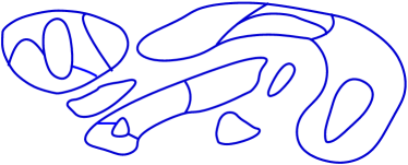
Figure 8: A typical configuration in the spin-$1$ loop model

The lines in this figure represent “spin-$1$” particles, so that they correspond to the projected double lines in the earlier Figs. 6 and 7. We thus dub this the spin-$1$ loop model. We still require that the strands form closed loops. However, as opposed to the $SU(2)$ case, we must now allow for trivalent vertices, i.e. the loops are now allowed to branch and merge. Thus the spin-$1$ loop model has branching loops, i.e. the configurations are netslevin03 . In the language of the quantum-group algebra $U_{q}(sl_{2})$, the reason for the trivalent vertices is that spin $1$ appears in the tensor product of two spin-$1$ representations. Equivalently, one can form an invariant from three spin-$1$ representations. Pictorially, this follows from the presence of the $SO(3)$ BMW generator $X$ in Fig. 7. This generator does not occur in the $SU(2)$ case. In the quantum-group language, there are three generators here because the three representations of spin $0,1$ and $2$ appear in the tensor product of two spin-$1$ representations. Precisely, the projection of two spin-1 strands onto a spin-zero strand is $E/(Q-1)$, and onto a spin-1 strand is $(X-E)/(Q-2)$.

In the spin-$1/2$ loop model for the lattice $O(n)$ model freedman04 , the Temperley-Lieb relation $e_{i}^{2}=de_{i}$ implies that each loop receives a weight $d$. We can understand the somewhat more intricate analogous properties of the spin-$1$ loop model by using the $SO(3)$ BMW algebra. The relation $E_{j}^{2}=(Q-1)E_{j}$ implies that isolated loops in the spin-$1$ model receive a weight of $Q-1=d^{2}-1$. Because trivalent vertices occur here, however, all loops need not be isolated. The projector onto spin-$1$ is proportional to $X-E$, so we associate this with two neighboring trivalent vertices, as indicated in Fig. 9.

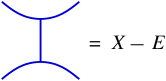
Figure 9: Two trivalent vertices in the $SO(3)$ BMW algebra

Several properties of the loop gas follow from this. The relation $(X_{j}-E_{j})^{2}=(Q-2)(X_{j}-E_{j})$ means that a configuration with a loop with just two lines emanating from it has a weight $Q-2$ times the configuration with the loop removed. This is illustrated in Fig. 10.

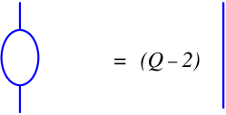
Figure 10: Removing one loop in the spin-1 loop model

Moreover, because $(X_{j}-E_{j})E_{j}=0$, no graph can contain any loop with just one external line attached to it. We call such a forbidden loop a “tadpole”.

We must work harder to find the weight of more complicated configurations in the loop model. To make the answer precise, we use a two-dimensional classical lattice model which has a loop expansion with the desired properties. As we discussed in Section V, for the spin-$1$ loop model this should be the $Q$-state Potts model, since its $S$ matrix gives the desired braid matrix. The desired loop expansion is the low-temperature expansion of the Potts model.

Let us first describe the low-temperature loop expansion for $Q$ integer, where the Potts models are defined by placing a “spin” $\sigma_{i}$ taking values $1\dots Q$ at the sites $i$ of a lattice. As it is well known, the interaction for a Potts model depends only on whether nearest-neighbor spins are the same or different, so that the Boltzmann weight for a link with spins $\sigma_{i}$ and $\sigma_{j}$ at its ends is

$$e^{K(\delta_{\sigma_{i}\sigma_{j}}-1)}.$$

The low-temperature expansion is given by first expressing each configuration of Potts spins in terms of its domain walls. The domain walls reside on the links of the dual lattice, and separate regions on the direct lattice of spins of different values. Each link crossing a domain wall has weight $e^{-K}$, while each link without a domain wall has weight $1$. The Boltzmann weight of a given spin configuration depends only on the length $L$ of its domain walls: $L$ is the number of links on the dual lattice with walls on them. The Boltzmann weight of a configuration is then $e^{-KL}$. A weight of $1$ per unit length corresponds to infinite temperature in this classical lattice model.

By definition, the domain walls must form loops surrounding groups of like Potts spins. These loops can intersect, but no tadpoles can occur. For example, the trivalent vertex given in Fig. 11 occurs for $Q>2$.

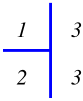
Figure 11: A trivalent vertex in the 3-state Potts model

Different configurations of spins can have the same domain-wall configuration: e.g. there are $Q$ configurations with no domain walls, and $Q(Q-1)$ configurations with a loop of length $4$ surrounding a given site. In general, the number of spin configurations which have the same loop configuration ${\cal L}$ is called the number of $Q$-colorings $\chi_{Q}({\cal L})$ (see e.g. Ref. FK, ). Imagine each region of like spins to be shaded some color. The number $\chi_{Q}$ is then the number of ways this shading can be done with $Q$ colors so that no two adjacent regions have the same color (regions which meet only at a point are not considered to be adjacent).

The partition function of the Potts model can therefore be written as

$$Z=\sum_{\cal L}e^{-KL}\chi_{Q}({\cal L})$$ (21)

where the sum is over all distinct loop configurations: the multiple spin configurations with the same loop configuration is accounted for by the factor $\chi_{Q}({\cal L})$. A typical loop configuration ${\cal L}$ looks like that in fig. 8. Because $\chi_{Q}({\cal L})$ vanishes for any configuration with a tadpole, or a strands with dangling end, we need not include such configurations in the sum. This expansion is a useful description of the ferromagnetic ($K>0$) Potts model at low temperature. It is important to note that this is not the only loop expansion of the Potts model: another expansion is in terms of the (self- and mutually-avoiding) loops surrounding the clusters in the high-temperature expansion. FK ; nienhuis ; saleur .

The low-temperature expansion of the partition function of the Potts model, Eq.(21), applies to any $Q$ when $\chi_{Q}({\cal L})$ is the chromatic polynomial of the graph dual to ${\cal L}$.pottsnew The graph dual to ${\cal L}$ is defined with a node corresponding to each loop, and a line between two nodes when the corresponding loops share a boundary. In terms of the Potts spins, each node in this graph corresponds to a region of like spins, and a line between two nodes means that corresponding regions are adjacent. The chromatic polynomial reduces to the number of colorings of the graph when $Q$ is an integer, but can be defined for all $Q$ by a recursion relation. Consider two nodes connected by a line $l$ (i.e. two loops sharing a boundary in the original picture). Then define ${\cal D}_{l}{\cal L}$ to be the graph with the line deleted, and ${\cal C}_{l}{\cal L}$ to be the graph with the two nodes joined into one. Then we have

$$\chi_{Q}({\cal L})=\chi_{Q}({\cal D}_{l}{\cal L})-\chi_{Q}({\cal C}_{l}{\cal L}).$$ (22)

We represent this pictorially in fig. 12, where a node represents each loop, a solid line between two nodes indicates that the corresponding two loops are adjacent, and a dashed line indicates that two formerly independent loops are now merged (i.e. the occupied links separating them are removed).

Figure 12: The recursion relation for the chromatic polynomial

This is fairly obvious in the coloring description: $\chi_{Q}({\cal D}_{l}{\cal L})$ includes all graphs in $\chi_{Q}({\cal L})$, but also has graphs where the two nodes connected by line $l$ have the same color. There are $\chi_{Q}({\cal C}_{l}{\cal L})$ of the latter so we need to subtract these off to get the recursion relation. For any loop configuration ${\cal L}$, one can apply (22) repeatedly until one reaches graphs with all isolated nodes. A graph with ${\cal N}$ isolated nodes has $\chi_{Q}=Q^{\cal N}$. We will give explicit examples of how this works in Subsection VI.2.

The criteria for the Potts loop model to describe the ground state of the $SO(3)$ loop gas on the lattice are therefore

$1^{\prime}$. The strands form closed loops, but now we allow trivalent vertices.

$2^{\prime}$. If two configurations are related by moving strands around without cutting the strands or crossing any other strands, then these two configurations must have the same weight. In other words, two topologically identical configurations have the same weight.

$3^{\prime}$. Each loop configuration ${\cal L}$ receives a weight $\chi_{Q}({\cal L})$. For example, if two configurations are identical except for one having a closed loop around a single plaquette (a loop of length 6 on the honeycomb lattice, length 4 on the square), then the weight of the configuration without the single-plaquette loop is $Q-1$ times that of the one with it.

Criterion $2^{\prime}$ is the same as criterion $2$ in the $SU(2)$ case; this is the requirement of topological invariance. Criterion $1^{\prime}$ is the generalization of criterion $1$, allowing for trivalent vertices in the $SO(3)$ case. Criteria $3^{\prime}$ is the appropriate generalization of criterion $3$. However, implementing this using a local Hamiltonian requires a little work, which we will now describe.

VI.2 A Hamiltonian yielding $SO(3)$ statistics

In the previous Subsection we set out the criteria which the ground-state wave function for the $SU(2)$ and $SO(3)$ models must obey. Here we describe a Hamiltonian of the form of Eq.(20) for the $SO(3)$ case, which has a ground state with the weights of the (low-temperature) Potts loop gas. This is tantamount to finding a set of projection operators $H_{i}$ which annihilate the desired ground state, and which result in an ergodic Hamiltonian.

There are two types of $H_{i}$ operators in our Hamiltonian. The simplest type have purely potential terms, diagonal terms where $H_{i}=1$ on some basis elements of the Hilbert space, and zero on the remaining elements. Such terms thus allow us to satisfy criterion $1^{\prime}$: we give a positive potential to any vertex which has only one occupied link touching it. Since the ground state has energy zero by construction, any state on which these $H_{i}$ are non-zero cannot be part of the ground state, as long as there are no off-diagonal terms which mix this state with an allowed one.

The second type of term contains off-diagonal elements, and are needed to ensure that different basis elements have the desired relative weighting in the ground state. A state of the form $|{\cal L}\rangle+\alpha|{\cal L}^{\prime}\rangle$ is annihilated by

$$H_{i}=\begin{pmatrix}\alpha&-1\\ -1&\alpha^{-1}\end{pmatrix}$$ (23)

so that e.g. $H_{i}|{\cal L}\rangle=\alpha|{\cal L}\rangle-|{\cal L}^{\prime}\rangle$. Since we know each state ${\cal L}$ in the ground state receives a weight $\chi_{Q}({\cal L})$, we need $\alpha=\chi_{Q}({\cal L}^{\prime})/\chi_{Q}({\cal L})$.

However, if we include an element $H_{i}$ in the Hamiltonian for any pair of states ${\cal L},{\cal L}^{\prime}$, the Hamiltonian will be non-local for several reasons. An obvious one is that if we include an $H_{i}$ for any pair of configurations, the off-diagonal terms are clearly non-local. We can easily solve this problem by setting $\lambda_{i}=0$ for any $H_{i}$ involving an ${\cal L}$ and a ${\cal L}^{\prime}$ whose differences are non-local. In other words, we only allow off-diagonal terms in $H$ which map a given ${\cal L}$ to an ${\cal L}^{\prime}$ which differs from ${\cal L}$ only in some small neighborhood (say the links on a given plaquette). While this is a necessary condition for a local Hamiltonian, it is not sufficient for this model. The reason is that evaluating $\chi_{Q}({\cal L})$ for a given ${\cal L}$ is a non-local operation: it requires knowing the entire cluster of occupied links. However, even though the overall $\chi_{Q}({\cal L})$ needs to be determined globally, the ratio $\chi_{Q}({\cal L})/\chi_{Q}({\cal L}^{\prime})$ in some cases depends only on local difference between ${\cal L}$ and ${\cal L}^{\prime}$, not their global form. Since the Hamiltonian only depends on this ratio, we can find a local Hamiltonian if we can find such pairs ${\cal L}$ and ${\cal L}^{\prime}$.

Let us first describe how to implement criterion $2^{\prime}$, which says that if two configurations ${\cal L}$ and ${\cal L}^{\prime}$ are topologically identical, then they have the same weight in the ground state. By definition, if ${\cal L}$ is topologically identical to ${\cal L}^{\prime}$, we have $\chi_{Q}({\cal L})=\chi_{Q}({\cal L}^{\prime})$. Thus including $H_{i}$ of the form of Eq.(23), with $\alpha=1$ will insure the proper weighting. These terms will be local if we require ${\cal L}$ and ${\cal L^{\prime}}$ to not only be topologically identical, but completely identical except on the links around one plaquette.

To make these terms in the Hamiltonian more specific, let us work henceforth on the honeycomb lattice, so that we do not have to worry about loops which touch at only a point. Consider a single plaquette, where some but not all of its six links are occupied. The simplest possibility allowed by criterion $1^{\prime}$ is then for two of the six outside links touching the plaquette to be occupied, as in all the configurations in Fig. 13.

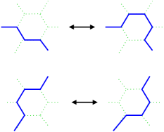
Figure 13: Plaquettes with two external occupied links

For each configuration of the two outside occupied links (15 possibilities in all), there are two topologically-identical configurations on each plaquette. We thus include in $H$ the $\alpha=1$ projectors which include flips between the two topologically-identical configurations; two of the flips are illustrated in Fig. 13. These $H_{i}$ are local, involving only states on 12 links: the six on the plaquette and the six touching it.

This idea can readily be generalized to plaquettes with more of the outside links occupied. If there are three outside links occupied, then there are three topologically-identical configurations on each plaquette, as illustrated in one case in Fig. 14.

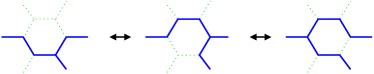
Figure 14: Plaquettes with three external occupied links

We thus include $\alpha=1$ projectors which flip between any pair of topologically-identical configurations. For four outside lines, there are two possibilities. The first type of configuration shown in Fig. 15 has no topologically-identical partner, while the second type has one.

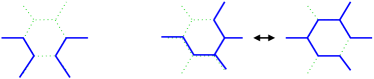
Figure 15: Plaquettes with four external occupied links

We thus include $\alpha=1$ projectors for all configurations of the latter type. For five or six outside lines, we include no projectors. By repeatedly applying the $H_{i}$ described in Figs. 13, 14 and 15, we implement criterion $2^{\prime}$.

As if this Hamiltonian weren’t already complicated enough, we now need to implement criterion $3^{\prime}$. The $H_{i}$ described in Figs. 13 all map between topologically-identical configurations. To map between topologically-distinct configurations, we need still more $H_{i}$ operators. These are still of the form of Eq.(23), but to ensure different configurations have the correct relative weight, the $\alpha$ are not necessarily equal to $1$. Again, we focus on a single plaquette, but here we consider only plaquettes with all six links occupied. The $H_{i}$ depend of course on which of the outside links are occupied. The cases with $0$, $1$, $2$, and $3$ occupied outside links and all internal links occupied are easy to implement. We have:

0. When there are no outside links occupied, then a plaquette with all six links occupied forms an isolated loop. If we remove this loop, the resulting configuration has weight $Q-1$ relative to the configuration with the loop. This can be implemented with an $H_{i}$ with $\alpha=Q-1$, where ${\cal L}$ is the configuration with the isolated loop and ${\cal L}^{\prime}$ is the configuration without it. This is illustrated in fig. 16.

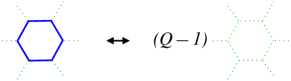
Figure 16: Removing or adding an isolated loop

1. If there is just one occupied link, this is a tadpole, and is forbidden in the Potts loop expansion and hence the ground state. Thus we add a potential-only term (i.e. $H_{i}=1$ on a tadpole). Tadpoles comprised of loops larger than a plaquette end up being forbidden by using the isotopy: applying the Hamiltonian enough will shrink a given loop to a single plaquette, and potential here will then exclude it from the ground state.

2. If there are two occupied outside links connected to loop, the configuration with the loop removed has relative weight $Q-2$, as illustrated earlier in Fig. 10. This is implemented by $H_{i}$ with $\alpha=Q-2$, where ${\cal L}$ is the configuration with the loop, and ${\cal L}^{\prime}$ is a configuration with the same external lines but without the complete loop. As illustrated in Fig. 13, for a given pair of occupied outside links, there are two allowed configurations on the plaquette with no loop. We can include a $H_{i}(\alpha=Q-2)$ for either or both of these two allowed configurations.

3. If there are three occupied outside links connected to loop, the configuration with the loop removed has relative weight $Q-3$. We therefore use an $H_{i}$ with $\alpha=Q-3$. Here ${\cal L}^{\prime}$ can be any one of the three configurations illustrated in Fig. 14.

A Hamiltonian comprised of the $H_{i}$ we have constructed so far has ground states with the correct relative weightings. However, it is not ergodic: there are multiple distinct ground states which are not related by any of the above off-diagonal terms. For example, a configuration with four adjacent plaquettes with all six links occupied, as illustrated in Fig. 17 below, is annihilated by all the $H_{i}$ we have discussed so far. Thus we need more terms in $H$ so that this state alone is not a ground state. Removing one of these loops (all of which have at least four occupied outside links) is not as simple as with three or less occupied links. We need to use the recursion relation Eq.(22) for the chromatic polynomial to find $H_{i}$ which remove these loops.

To find these terms, it is convenient to use the graphical representation of a loop configuration, as defined above. Knowing the graph of ${\cal L}$ is sufficient to find its chromatic polynomial $\chi_{Q}({\cal L})$. In terms of these graphs, the recursion relation Eq.(22) can be represented as in Fig. 12 above. We can use this relation to easily rederive the $H_{i}$ acting on plaquettes with $0$, $2$ and $3$ occupied outside links. For example, the graph for an isolated node is precisely that on the left-hand-side of Fig. 12. Applying Eq.(22) once, and then using the fact that an isolated node gives a factor $Q$ to the chromatic polynomial, gives the desired relative weighting $Q-1$. The equalities are meant as between the corresponding chromatic polynomials.

Finding $H_{i}$ which remove a loop with four external lines is trickier. One can apply the recursion relation, but one can get graphs which do not correspond to any configuration on the honeycomb lattice given by changing links on the plaquette from occupied to unoccupied. Consider the first graphical representation of four adjacent hexagons in Fig. 17.

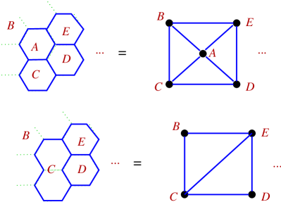
Figure 17: Graphical representations of two configurations with five loops

In this graph, we allow the nodes $B$, $C$, $D$ and $E$ to be attached to other nodes, but node $A$ touches only the four in the picture. We apply the recursion relation once to remove one of the lines attached to node $A$. This gives a perfectly valid relation for the corresponding chromatic polynomials, but there is no loop configuration corresponding to the graph with one line removed. For example, say we remove the line from $A$ to $D$: no loop configuration corresponding to this graph can be drawn on the honeycomb lattice.

To define a Hamiltonian, we need a relation between valid loop configurations, not just different chromatic polynomials. We can relate the two loop configurations in Fig. 17. In the first graph, we use the recursion relation to remove the line from $A$ to $D$ and then the line from $A$ to $E$. Now node $A$ has lines only to nodes $B$ and $C$, and corresponds to the situation of Fig. 10. We can now remove node $A$ altogether, multiplying the result (the square involving $B,C,D$ and $E$) by $Q-2$. This square defines a chromatic polynomial, but there is no corresponding loop configuration. We can however, relate it to the second configuration in Fig. 17; the same square graph arises from using the recursion relation to remove the link from $C$ to $E$. Combining the two, we obtain the relation in Fig. 18 with $a=Q-2$ and $b=-1$.

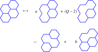
Figure 18: Removing one loop of a four-hexagon cluster

Note that the first and last configurations are topologically identical, so we can choose any value of $a$ if we set $b=Q-3-a$. Thus a more symmetric Hamiltonian will result if we choose $a=b=(Q-3)/2$. As a check on this relation, we can look at the special case where none of the nodes $A,C,D,E$ are connected to any others (i.e. the four hexagons $A,C,D,E$ are surrounded by region $B$). One can then easily verify that both sides are equal to $(Q-1)(Q-2)(Q-3)^{2}$.

We can then include an $H_{i}$ with ${\cal L}^{\prime}$ the sum of loop configurations on the right-hand-side of Fig. 18. One can define analogous relations to define new ${\cal H}_{i}$ which further reduce the number of loops on the right-hand-side of Fig. 18. Although we have not proven so, we believe that proceeding in this fashion one can define local $H_{i}$ which result in an ergodic Hamiltonian. This should also be possible on other lattices, but presumably be even more complicated, since one must worry about loops which touch at only a point. Obviously, there is no conceivable way such finely-tuned Hamiltonians could be realized in nature. However, the fact that they are local makes it at least possible that there exists a more natural Hamiltonian in the same universality class.

VII The phase transition

Since we have identified the classical field theories which describe the ground state of the quantum loop gas, we can determine the phase structure of the latter. There is a major subtlety in doing so. So far, we have been discussing properties of the wave function $\psi$. However, in determining equal-time correlation functions of the quantum system, the functional integral is weighted by $|\psi|^{2}$. In terms of the action of the corresponding classical model, we have from Eq.(12),

$$|\psi(s)|^{2}=e^{-S(s)-S^{*}(s)}$$

for a configuration $s$ in the classical model. Thus when we are computing for example correlators in the quantum model, we need to square the Boltzmann weights of the classical model. In a model where the loops themselves are the degrees of freedom (such as those discussed in Section VI, the ones without the Jones-Wenzl projector imposed), this means the weight per loop must be squared. In particular, this means loops in the $SU(2)$ model get weight $d^{2}$, while isolated loops in the $SO(3)$ model have weight $(d^{2}-1)^{2}$.

The phase structure depends on the weight per length of the loops. Let us first review what happens in a quantum eight-vertex model kitaev ; ardonne . There the degrees of freedom in the ground state are arrows on the links of the square lattice obeying the eight-vertex condition (an even number of arrows pointing in at each vertex). The loops are given by following (say the up and right-pointing) arrows around the lattice; the eight-vertex condition ensures the loops are closed. One can rewrite these degrees of freedom as Ising spins at the center of each plaquette, and the loops then form domain walls around the spins. The purely topological (Kitaev) pointkitaev , corresponding to our $SU(2)_{1}$ and $O(3)_{2}$ models, has equal amplitude for all configurations. This is indeed infinite temperature for the Ising spins. By including a weight per length of the loop, one can move away from the Kitaev point. As detailed in Ref. ardonne, , there is eventually a phase transition to an ordered phase.

The interesting question to answer is if this is a critical point or a first-order phase transition. In the quantum eight-vertex model of Ref. ardonne, , the transition is second order. In the analogous transition in the $SU(2)$ case freedman01 ; freedman03 , each loop will get a weight $d^{2}$, so we can view this as a loop model with $n_{\rm eff}=d^{2}$. The $O(n_{\rm eff})$ model has a critical point only when $n_{\rm eff}=4\cos^{2}(\pi/(k+2))\leq 2$, so this occurs only for $k=1$ and $k=2$. Only the latter is non-Abelian.

The analogous result in the classical Potts model is that the phase transition at the self-dual point is second-order if $Q\leq 4$, first-order for $Q>4$. This result, however, cannot instantly be applied to the 2+1-dimensional case, because of the weighting by $|\psi|^{2}$: the phase structure is that of the classical loop gas where each configuration is weighted by $(\chi_{Q}({\cal L}))^{2}$. This loop gas does not seem to have been studied before, so we do not know the answer. However, we can make a simple conjecture. The configurations of this squared loop gas are of course the same as those of the Potts loop gas; only the weight per loop has been squared. One might therefore hope that the phase transition of the squared loop gas is in the same universality class as the Potts loop gas at some $Q_{\rm eff}$. The simplest possibility is to assume that $Q_{\rm eff}$ gives isolated loops in the squared loop gas the correct weight $(Q-1)^{2}$. This amounts to a $Q_{\rm eff}$ of

$$Q_{\rm eff}-1=(Q-1)^{2}=(d^{2}-1)^{2}.$$ (24)

The weight per unit length is also changed, but this only changes the location of the critical point, not its type. Thus we conjecture that there will be a critical point in the quantum loop gas if $Q_{\rm eff}\leq 4$, and a first-order transition otherwise.

If this conjecture is true, critical points occur for $k=2,3$ in the $SO(3)$ model (as noted above, $k=1$ is a trivial theory here). The $k=3$ model has non-Abelian statistics. As noted at the end of section II.3, this “Lee-Yang” model is the simplest model of non-Abelian statistics, since it has only one kind of strand. We have thus shown that in the quantum loop gas which realizes particles with these statistics, there exists a critical point separating the topological phase from an ordered one.

However, there’s a catch. The Jones-Wenzl projector needs to be imposed separately to the loop models discussed in Section VI, at least when space is an annulus or a torus. This presumably amounts to a relevant operator at the critical point freedman04 . Thus in the non-Abelian case even at $k=3$, reaching the critical point from the topological phase requires tuning another parameter away.

This is in harmony with some of our early observations. At the end of Section II.2 we noted that for the $SO(3)$ model with $k=3$, one can use the Jones-Wenzl projector to remove $X$ vertex, leaving only self-avoiding loops. The $SO(3)_{3}$ model with the projection is therefore equivalent (at least locally) to the $SU(2)_{3}$ model. The latter does not have a critical point, even without the Jones-Wenzl projector, because $k=3$ in $SU(2)$ case corresponds to an $O(n_{\rm eff})$ loop model with $n_{\rm eff}>2$. This is a strong indication that imposing the Jones-Wenzl results in a relevant perturbation of the critical theory.

Appendix A The Landau-Ginzburg description of the 1+1-dimensional theories

In this appendix we explain how the field theories discussed in section V, and their $S$ matrices discussed in section IV, have a nice description in terms of a Landau-Ginzburg effective field theory.

As shown in Ref. ZamoLG, , a simple Landau-Ginzburg description of the minimal model of conformal field theory with central charge of Eq.(19) is in terms of a single scalar field $\phi$ with potential $\phi^{2(p-1)}$. The critical point of the Ising model is the $p=3$ case, and the tricritical point is the $p=4$ case, and the corresponding $\phi^{4}$ and $\phi^{6}$ potentials have long been known. The critical point of the $SU(2)_{k}$ case (the continuum limit of the $O(n)$ or restricted height models) has $p=k+2$. The critical point of the $SO(3)_{k}$ case (the continuum limit of the Potts or dilute $A_{k+1}$ models) has $p=k+1$.

The primary fields of the conformal field theory also can be described in terms of $\phi$, so the massive field theories of interest have a Landau-Ginzburg description as well. For the $SU(2)_{k}$ case, the effective description of the $\Phi_{1,3}$ operator is $\phi^{2(p-2)}$. For the Ising model, this is indeed the usual $\phi^{2}$ mass term. As is well known, this field theory has a single quasiparticle with $S=-1$. In this case, $e_{i}$ must act on a one-dimensional space, and it is just a number; for $p=3$, $e_{i}=1$. This also follows from imposing the Jones-Wenzl projector: for $k=1$, one imposes ${\cal P}^{(1)}_{i}(d=1)=I-e_{i}=0$, which indeed gives $e_{i}=I$. Thus the statistics for $SU(2)_{1}$ is Abelian freedman01 ; freedman03 .

For higher values of $p$, perturbing a $\phi^{2(p-1)}$ potential by $\phi^{2(p-2)}$ seems to induce a flow to the minimal model with $p$ decreased by $1$. This flow is indeed known to occur for perturbations of one sign of $\Phi_{1,3}$, see Ref. ludwigcardy, . In the $O(n)$ language, this perturbation corresponds to flowing into the dense phase. In the models of Ref. ABF, this is called regime IV. This is not what we want; this is a massless field theory with the problematic $S$ matrix. Instead, we want to perturb by the same operator $\Phi_{1,3}$ but with the opposite sign; the perturbations are not the same because there is no symmetry in the conformal field theory (except in the Ising case) which sends $\Phi_{1,3}$ to $-\Phi_{1,3}$. With this sign of the perturbation, the potential must renormalize to include extra terms. Since we know from the exact resultsABF ; Huse that the lattice models have $p-1$ ground states, we must fine-tune the potential to achieve this. This is very familiar from the tricritical Ising model $p=4$. One sign of the perturbation moves the system along its first-order transition line, while the other sign causes a flow to the ordinary Ising critical point. The Landau-Ginzburg potential along the first-order line indeed consists of a $\phi^{6}$ potential tuned to have three degenerate minima.

Let us focus on $p=4$ case in more detail. The Landau-Ginzburg potential for the tricritical Ising model along its first-order transition line along is $\phi^{6}+a\phi^{4}+b\phi^{2}$, with $b=-6a^{2}$ so that there are three degenerate minima at $\phi=0,\pm\sqrt{2a}$. With such a potential, the low-energy configurations in the two-dimensional classical model consist of regions of these three vacua. The loops are domain walls between different vacua. When there are restrictions on which vacua can be adjacent to each other, the allowed domain walls are restricted as well. What happens here is that the vacuum $+\sqrt{2a}$ is not allowed to be next to the vacuum $-\sqrt{2a}$. Hence, there must be a region of vacuum $0$ in between. In the 1+1-dimensional description in terms of quasiparticles, the particles are kinks interpolating between adjacent vacua, and the domain walls are their world lines.

One can now count the “number” of particles. Say the left end of the system is in the vacuum $0$. Then the space of states for one particle $V(1)$ is two-dimensional; it consists of a kink going from $0$ to $+\sqrt{2a}$, and one going from $0$ to $-\sqrt{2a}$. However, the space $V(2)$ is also two-dimensional: the reason is this restriction that the two vacua $\pm\sqrt{2a}$ cannot be next to each other. Thus, if we have a kink going from $0$ to $+\sqrt{2a}$, the next kink can only go back to $0$ again. The dimension of the allowed Hilbert space for $N$ “particles”, $V(N)$ (with the boundary condition of vacuum 0 at one end), is therefore $2^{[(N+1)/2]}$, where $[x]$ is the integer part of $x$.This reduction of the Hilbert space, with respect to the standard free particle Fock space, is the hallmark of non-Abelian statistics. Using the standard definition of the “number of particles” as ln(dim$(V(N)))/N$, here we find $\sqrt{2}$ This is indeed the correct value of $d$ for $k=2$, and gives a precise meaning to the statement that $d$, the weight per loop, can be interpreted as counting the “number of particles going around a given loop” (albeit this “number” is $\sqrt{2}$ !).

Thus we see how these restricted kinks in 1+1 dimensions go hand-in-hand with non-Abelian statistics in 2+1 dimensions. In the Moore-Read theory of the $\nu=5/2$ fractional quantum Hall effect moore92 , the quasiparticles have non-Abelian statistics, and the number of states obeys the same formula $2^{[N/2]}$, where $N$ here is the number of quasiholes (“non-abelions”) nayak .

For general $SU(2)_{k}$ theories, we consider a $\phi^{2(k+1)}$ potential with $k+1$ minima. (The explicit potential can be written out in terms of Chebyshev polynomials if desired.) The kinks interpolate between adjacent vacua, so that their world lines are domain walls in the two-dimensional picture. To count the “number” of such kink configurations for large $N$, one applies the same procedure as above, and obtains $2\cos^{N}(\pi/(k+2))$. In the Read-Rezayi generalizations of the Moore-Read theory of the fractional quantum Hall effect read-rezayi , the statistics and the number of states is the same slingerland .

For the $O(3)_{k}$ case, the perturbation of the conformal minimal model is different. The $\Phi_{21}$ operator is $\phi^{p-1}$, but the resulting Landau-Ginzburg description is not as useful. However, in section II we showed how to describe representations of the $SO(3)$ BMW algebra by fusing together representations of the Temperley-Lieb algebra, and the analog is possible here. We can describe the kinks in the Potts models as bound states of the kinks of the $O(n)$ model, although we believe that in the $S$ matrix context this is a formal device without physical significance. Anyway, we consider the same potential with $k+1$ degenerate minima, but the $O(3)_{k}$ kinks are comprised of two of the $SU(2)_{k}$ kinks. More precisely, we consider all configurations made up of two $SU(2)_{k}$ kinks bound together, and then subtract off the identity. This procedure yields the correct fusion rules for spin-1 particles, and the correct “number” of kinks $d^{2}-1$.

References

- (1) R.B. Laughlin, Phys. Rev. Lett. 50, 1395 (1983).
- (2) D. Arovas, J.R. Schrieffer and F. Wilczek, Phys. Rev. Lett. 53, 722 (1984).
- (3) F.E. Camino, W. Zhou and V.J. Goldman, “Direct observation of fractional statistics in two dimensions”, [arXiv: cond-mat/0502406]
- (4) G. W. Moore and N. Read, Nucl. Phys. B 360, 362 (1991).
- (5) A.Y. Kitaev, Ann. Phys (N.Y.) 303, 2 (2003) [arXiv:quant-ph/9707021]
- (6) M. Freedman, Comm. Math. Phys. 234, 129 (2003) [arXiv: quant-ph/0110060].
- (7) M. Freedman, C. Nayak, K. Shtengel, K. Walker and Z. Wang, Ann. Phys (N.Y.) 310, 428 (2004) [arXiv: cond-mat/0307511].
- (8) S. C. Zhang and T. H. Hansson and S. A. Kivelson, Phys. Rev. Lett. 62, 82 (1989); A. López and E. Fradkin, Phys. Rev. B 44, 5246 (1991)
- (9) X.G. Wen and A. Zee, Phys. Rev. B 46, 2290 (1992); J. Fröhlich and A. Zee, Nucl. Phys. B 364, 517 (1991).
- (10) X.G. Wen, Adv. in Phys. 44, 405 (1995).
- (11) E. Witten, Comm. Math. Phys. 121, 351 (1989).
- (12) P.W. Anderson, Science 235, 1196 (1987).
- (13) S.A. Kivelson, D. Rokhsar and J. Sethna, Phys. Rev. B 35, 865 (1987).
- (14) D. S. Rokhsar and S. A. Kivelson, Phys. Rev. Lett. 61, 2376 (1988)
- (15) R.Moessner and S.L. Sondhi, Phys. Rev. Lett. 86, 1881 (2000) [arXiv: cond-mat/0007378]
- (16) S.A. Kivelson, Phys. Rev. B 36, 7237 (1987)
- (17) N. Read and B. Chakraborty, Phys. Rev. B 40, 7133 (1989)
- (18) N. Read and S. Sachdev, Phys. Rev. Lett. 66, 1773 (1991); S. Sachdev and N. Read, Int. J. Mod. Phys B 5, 219 (1991) [arXiv: cond-mat/0402109]
- (19) T. Senthil and M.P.A. Fisher, Phys. Rev. B 62, 7850 (2000) [arXiv: cond-mat/9910224]
- (20) N. Read and E. Rezayi, Phys. Rev. B 59, 8084 (1999) [arXiv: cond-mat/9809384]
- (21) E. H. Fradkin, C. Nayak and K. Schoutens, Nucl. Phys. B 546, 711 (1999) [arXiv:cond-mat/9811005].
- (22) E. Ardonne and K. Schoutens, Phys. Rev. Lett. 82, 5096 (1999) [arXiv: cond-mat/9811352].
- (23) D.A. Ivanov, Phys. Rev. Lett. 86, 268 (2001) [arXiv: cond-mat/0005069]
- (24) M.G. Alford, K.M. Lee, J. March-Russell and J. Preskill, Nucl. Phys. B 384, 251 (1992) [arXiv:hep-th/9112038].
- (25) H.K. Lo and J. Preskill, Phys. Rev. D 48, 4821 (1993) [arXiv:hep-th/9306006].
- (26) M. de Wild Propitius and F.A. Bais, “Discrete Gauge Theories ” [arXiv:hep-th/9511201]
- (27) E. Witten, Comm. Math. Phys. 144, 189 (1992).
- (28) G. Grignani, G. W. Semenoff, P. Sodano and O. Tirkkonen, Nucl. Phys. B 489, 360 (1997) [arXiv:hep-th/9609228].
- (29) E. Ardonne, P. Fendley and E. Fradkin, Ann. Phys (N.Y.) 310, 493 (2004) [arXiv:cond-mat/0311466].
- (30) M. Freedman, C. Nayak and K. Shtengel, “A line of critical points in 2+1 dimensions: Quantum critical loop gases and non-Abelian gauge theory,” [arXiv:cond-mat/0408257].
- (31) M. Freedman, C. Nayak and K. Shtengel, “An extended Hubbard model with ring exchange: a route to a non-Abelian topological phase,” [arXiv:cond-mat/0312273]; “Non-Abelian topological phases in an extended Hubbard model,” [arXiv: cond-mat/0309120].
- (32) H. Temperley and E.H. Lieb, Proc. Roy. Soc. (London) A322, 251 (1971).
- (33) C. Castelnovo, C. Chamon, C. Mudry, P. Pujol, “The quantum three-coloring dimer model and its line of critical points that is interrupted by quantum glassiness,” [arXiv: cond-mat/0410562]
- (34) M. A. Levin and X. G. Wen, Phys. Rev. B 67, 245316 (2003) [arXiv: cond-mat/0302460]; Phys. Rev. B 71, 045110 (2005) [arXiv: cond-mat/0404617]
- (35) B. Nienhuis in Phase Transitions and Critical Phenomena, ed. by C. Domb and J. Lebowitz, vol. 11, (Academic Press, 1987)
- (36) V. Jones, Invent. Math. 72, 1 (1983)
- (37) L. Kauffmann, Knots and Physics (World Scientific, 1991)
- (38) M. Wadati, T. Deguchi and Y. Akutsu, Phys. Rep. 180, 247 (1989).
- (39) S. Deser, R. Jackiw and S. Templeton, Ann. Phys (N.Y.) 140, 372 (1982) [Erratum-ibid. 185, 406 (1988)].
- (40) J. Murakami, Osaka J. Math. 24, 745 (1987); J. Birman and H. Wenzl, Trans. Amer. Math. Soc. 313, 239 (1989).
- (41) J.K. Slingerland and F.A. Bais, Nucl. Phys. B 612, 229 (2001) [arXiv:cond-mat/0104035].
- (42) P. Fendley and N. Read, J. Phys. A 35, 1 (2003) [arXiv:hep-th/0207176].
- (43) J. L. Cardy, Phys. Rev. Lett. 54, 1354 (1985).
- (44) D. Arovas and S. Girvin, Lectures presented at the Seventh International Conference on Recent Progress in Many Body Theories, Minneapolis, 26-30 August 1991, unpublished.
- (45) A. B. Zamolodchikov and Al. B. Zamolodchikov, Ann. Phys (N.Y.) 120, 253 (1979).
- (46) G. E. Andrews, R. J. Baxter and P. J. Forrester, J. Stat. Phys. 35, 193 (1984).
- (47) V. Pasquier, Nucl. Phys. B 285, 162 (1987).
- (48) C. Nayak and F. Wilczek, Nucl. Phys. B 479, 529 (2004) [arXiv: cond-mat/9605145]
- (49) M. Jimbo, Lett. Math. Phys. 10, 63 (1985).
- (50) D. A. Huse, Phys. Rev. B 30, 3908 (1984).
- (51) A. B. Zamolodchikov, Mod. Phys. Lett. A 6, 1807 (1991).
- (52) F. A. Smirnov, Phys. Lett. B 275, 109 (1992).
- (53) P. Fendley and H. Saleur, Nucl. Phys. B 388, 609 (1992) [arXiv:hep-th/9204094].
- (54) A.M. Polyakov and P.B. Wiegmann, Phys. Lett. B 141, 223 (1984); E. Fradkin, C. M. Naón and F. A. Schaposnik,Phys. Lett. B 200, 95 (1987); D.C. Cabra, E.F. Moreno and G.L. Rossini, Phys. Lett. B 437, 362 (1998).
- (55) P. Goddard, A. Kent and D. Olive, Phys. Lett. B 152, 88 (1985); Int. J. Mod. Phys. A 1, 303 (1986).
- (56) A.B. Zamolodchikov, in Fields, Strings and Quantum Gravity, eds H. Guo et al (Gordon and Breach, 1990); Al. B. Zamolodchikov, Nucl. Phys. B 358, 497 (1991).
- (57) F.A. Smirnov, Int. J. Mod. Phys. A 6, 1407 (1991).
- (58) V.S. Dotsenko and V.A. Fateev, Nucl. Phys. B 240, 312 (1984).
- (59) P. Fendley, unpublished.
- (60) L. Chim and A. B. Zamolodchikov, Int. J. Mod. Phys. A 7, 5317 (1992).
- (61) H.A. Kramers and G.H. Wannier, Phys. Rev. 60, 252 (1941).
- (62) R.J. Baxter, Exactly Solved Models in Statistical Mechanics (Academic Press, New York, 1982).
- (63) L.P. Kadanoff and H. Ceva, Phys. Rev. B 11, 3918 (1971).
- (64) E. Fradkin and L. Susskind, Phys. Rev. D 17, 2637 (1978).
- (65) V. A. Fateev, Int. J. Mod. Phys. A 6, 2109 (1991).
- (66) V.G. Turaev, “Quantum invariants of knots and 3-manifolds”, de Gruyter Studies in Mathematics, 18, (Berlin, Walter de Gruyter & Co., 1994); V. G. Turaev, Ya O. Viro, “State sum invariants of 3-manifolds and quantum 6j-symbols”, Topology 31, 865 (1992).
- (67) A.N. Kirillov and N.Y. Reshetikhin, “Representations of the algebra , -orthogonal polynomials and invariants of links”, in Infinite dimensional Lie algebras and groups, Proceedings of the conference held at CIRM, Luminy, Marseille, V.G. Kac editor, pages 285-339, World Scientific (Singapore, 1988); N. Reshetikhin, and V.G. Turaev, Invent. Math. 103, 547 (1991).
- (68) G. Kuperberg, Comm. Math. Phys. 180, 109 (1996) [arXiv: q-alg/9712003]
- (69) C.M. Fortuin and P.W. Kasteleyn, Physica 57, 536 (1972).
- (70) H. Saleur, Nucl. Phys. B 360, 219 (1991).
- (71) A. B. Zamolodchikov, Sov. J. Nucl. Phys. 46, 1090 (1987) [Yad. Fiz. 46, 1819 (1987)].
- (72) A. W. W. Ludwig and J. L. Cardy, Nucl. Phys. B 285, 687 (1987).