Multiple Scale-Free Structures in Complex Ad-Hoc Networks

Abstract

This paper develops a framework for analyzing and designing dynamic networks comprising different classes of nodes that coexist and interact in one shared environment. We consider ad hoc (i.e., nodes can leave the network unannounced, and no node has any global knowledge about the class identities of other nodes) preferentially grown networks, where different classes of nodes are characterized by different sets of local parameters used in the stochastic dynamics that all nodes in the network execute. We show that multiple scale-free structures, one within each class of nodes, and with tunable power-law exponents (as determined by the sets of parameters characterizing each class) emerge naturally in our model. Moreover, the coexistence of the scale-free structures of the different classes of nodes can be captured by succinct phase diagrams, which show a rich set of structures, including stable regions where different classes coexist in heavy-tailed (i.e., exponent is between 2 and 3) and light-tailed (i.e., exponent is $>3$) states, and sharp phase transitions. The topology of the emergent networks is also shown to display a complex structure, akin to the distribution of different components of an alloyed material; e.g., nodes with a light-tailed scale-free structure get embedded to the outside of the network, and have most of its edges connected to nodes belonging to the class with a heavy-tailed distribution. Finally, we show how the dynamics formulated in this paper will serve as an essential part of ad-hoc networking protocols, which can lead to the formation of robust and efficiently searchable networks (including, the well-known Peer-To-Peer (P2P) networks) even under very dynamic conditions.

I Introduction

I.1 Motivation

Real networks are rarely homogeneous, and often comprise different categories of constituent nodes, all of which interact and coexist in a single global environment. The classification of nodes in such networks might be based on different characteristics, including diverse functionalities, different objectives and scale of resources, and different types and degrees of dynamics inherent to the nodes. Examples include, different cell types in a neural network, different roles in the web of English words (e.g., verbs, nouns, and adjectives), different disciplines in the network of scientific collaborations, various switch types (routers, hubs, etc.) in the Internet, and the different node types in a Peer-to-Peer (P2P) network (e.g., nodes with 56K-Baud modem connections vs. nodes with DSL connections). Empirical evidence of class-specific hierarchical and scale-free structures in many complex networks have become available only recently hir . For example, a heterogeneous scenario has been reported in the network of scientific citations: While the overall structure of such networks is believed to have a power-law (PL) degree distribution with exponent $\gamma\approx 3$, the network of citations restricted to theoretical physicists is somewhat more heavy tailed with an exponent around $\gamma\sim 2.6$ the .

The objective of this paper is to explore the dynamics of such heterogeneous networks, and study how different types of nodes influence each other, and when and how multiple scale-free structures may emerge in the networks. We find that the interacting sets of different classes of nodes can give rise to a complex global structure, and display a rich set of emergent properties. In particular, we show (i) Viewing complex systems as networks with different evolving, and interacting constituent subnetworks, helps gain better understanding about the role of each class of nodes in the overall network, and sheds light on how different networks with nested structures might have evolved, and (ii) How the results can lead to the systematic design of heterogeneous networks, where different categories of nodes evolve to have different scale-free structures (corresponding to their capabilities and intentions).

I.2 Dynamical Model and Results

We consider ad hoc dynamical networks, where in addition to nodes joining the network, nodes also disconnect and leave the network randomly at certain rates. Moreover, nodes are allowed to respond to their environment, and can initiate new random connections if their existing connections are lost. The dynamical rules studied in this paper, have been picked from those traditionally studied in the context of complex networks. For example, in all the protocols studied in this paper all connections are initiated by choosing nodes in a linear preferential manner. Similarly, the other dynamics that we incorporate are joining of new nodes, random deletion of existing nodes, and compensatory rewiring by existing nodes that might have lost an edge because of the deletion dynamics. As described next, the different classes of nodes in the network follow the same global dynamics, except with different parameters. Additionally, to be true to the ad hoc nature of our model, we enforce that the class identity of a node is not a global knowledge; instead, a node’s identity is expressed only through its own dynamics and actions, i.e., in how it responds to and initiates contacts with other nodes in the network. Thus, a node on joining the network makes requests for connection without any global knowledge about the properties of other nodes in the network, and the connection requests are made following the traditional preferential attachment rule.

Modeling Heterogeneity of Nodes: The different classes of nodes are characterized by different sets of parameters they adopt in responding to connection requests, and also in executing local dynamics. The most important local parameters used in this paper to capture heterogeneity of nodes, include (i) attraction or attachment, i.e., a node’s willingness to accept a requested connection; this can be parametrized by the probability, $d_{q}$, with which the nodes in the $q^{th}$ class accept a connection request. (ii) stability, i.e., how long they stay in the network before dropping out or deleting themselves; this can be parametrized by the probability, $c_{q}$, with which a randomly picked node in the $q^{th}$ class gets deleted at each time step. (iii) responsiveness, i.e., a node’s ability to respond to lost or dead connections and compensate for them with new connection; this can be parametrized by the probability, $n_{q}$ with which a node in the $q^{th}$ class compensates for any lost or inactive connection, and (iv) representation or relative population, i.e., what percentage of the nodes joining the network belong to a specific class; this can be parameterized by the probability, $s_{q}$, with which a node joining the network is from the $q^{th}$ class. In general, the different categories of nodes in a network may differ in all four of these parameters.

I.3 Approach and A Preview of Results

We are interested in finding $P_{q}(k)$, the degree distributions within each of the subclasses. That is, $P_{q}(k)$ is the probability of a randomly chosen node of type $q$ to have degree $k$; note that all edges, both intra- and inter-community edges, contribute to the degree of a node. In particular, we will show the emergence of scale-free degree distributions within each class, that is $P_{q}(k)\propto k^{-\gamma_{q}}$. In general, for a given set of $Q$ classes, the PL exponent $\gamma_{q}$ of the $q^{th}$ class is a function of all the four sets of parameters. That is, in general we have

$$\gamma_{q}=f(D,C,N,S)\hbox{\hskip 11.38109pt for all $q=1,\ldots,Q$},$$

where $D=\{d_{1},\cdots,d_{Q}\}$, $C=\{c_{1},\cdots,c_{Q}\}$, $N=\{n_{1},\cdots,n_{Q}\}$, and $S=\{s_{1},\cdots,s_{Q}\}$, are the sets of, attachment, stability, responsiveness, and representation parameters for the $Q$ different classes of nodes. We apply the continuous-time rate equation approach to study the dynamics and derive $\gamma_{q}$’s. The coexistence of different classes of networks will impose certain constraints on the set of $\gamma_{q}$’s emerging in the subclasses, and hence, only certain sets of $\gamma_{q}$’s for a given choice of the dynamical parameters are feasible.

As discussed in Section IV, it is always possible to compute the $\gamma_{q}$’s numerically using the rate-equation approach. An exact closed form computation of the various PL exponents (as a function of the different sets of parameters), however, is difficult to obtain when the classes are heterogeneous with respect to all the local parameters. Hence, to develop intuition and to better understand the heterogeneous systems, we study special cases where it is possible to obtain exact formulas for the computation of $\gamma_{q}$’s. For example, in Section III we study the case, where the sets are heterogeneous over only the sets $D$ and $S$, i.e., the $q^{th}$ class has attachment rate $d_{q}$ and relative population $s_{q}$. Moreover, we allow deletions of random nodes at an overall rate of $c$ (i.e., the deletion rates of the $q^{th}$ class is given as $c_{q}=c*s_{q},$ and cannot be set independently), and no compensation, i.e., $n_{1}=n_{2}=\cdots=n_{Q}=0$. Eqs. 5 and III provide the exact formula for $\gamma_{q}$’s for this particular model. Interesting features include: (i) Coupled PL exponents: The average PL degree is constrained to be greater than $3$. Thus for example, for $Q=2$, one class can have PL exponent $<3$, while the other one has to have exponent $>3$. Recall that if $Q=1$ and $c=0$, it is exactly the case of linear preferential attachment, and the exponent is exactly equal to $3$. Hence, by having multiple classes, one can have classes that have heavy tailed PL degree distributions (i.e., exponent $<3$), even with the linear preferential attachment kernel. In general, for different $c$’s the possible PL exponents $(\gamma_{1},\gamma_{2})$ are plotted in Fig. 2. (ii) Role of the Deletion Rate $c$: If $Q=1$ then it is shown in us that for any deletion rate $c>0$, the PL exponent is $>3$, and that the exponent increases rapidly with an increase in $c$. As shown in Fig. 2, for two classes it is possible to have one class with PL exponent $<3$. However, there is always a deletion rate for which both the exponents become $>3$. Thus, the heterogeneity of the network can lead to rich structures, which otherwise do not exist in homogeneous networks.

The more general case, where we vary three sets of parameters, $C,N,S$, while the attachment rates are considered to be unity for all the classes, i.e., $d_{1}=\cdots=d_{Q}=1$, is considered in Section IV. It is best to describe the results in terms of a phase space, where the state of a class can be attributed as described in the following. Another means of studying the networks is to look at the embedding of the different classes of nodes in the overall structure. Both of these macroscopic approaches and related results are summarized in the following.

Emergence and Coexistence of Phases: The degree distribution of a particular category of node could be classified into the following phases or states, depending on the exponent, $\gamma$, of its PL distribution: (i) Heavy Tailed: $2\leq\gamma<3$; for such a distribution, the variance becomes unbounded while the mean remains bounded. It is in this regime that the corresponding network shows a number of advantageous properties, such as almost-constant diameter, efficiently searchable, and resistance to random deletions of nodes and edges. (ii) Light Tailed: $\gamma>3$, (iii) Unstable: $0<\gamma<2$, this is when the average degree becomes unbounded, and (iv) Extinction: when the average degree goes to zero, i.e., the nodes belonging to this class get disconnected from the rest. Clearly, one can make a finer division of the range of the PL exponent and define a larger number of phases.

We investigate issues related to how the different categories of nodes can be in different phases as a function of the parameters of the dynamics. Also, how will a phase transition within one subclass (e.g., from a heavy to a light tailed phase) affect the phase of the other classes? As shown in Section V, we find that the rich set of solutions of the dynamical model introduced in this paper, can be captured by succinct phase diagrams, which show the coexistence of different phases of different categories of nodes, as a function of the parameters. The results show that the phase space shows all the hallmarks of a rich heterogeneous system, including

• Stable regions where different categories of nodes can be in different desired phases (e.g., certain classes in the heavy-tailed phase, while certain others in the light tailed phase). These regions have sufficient volume/area so that the resulting degree-distributions are fairly insensitive to the exact choice of the different parameters; see simulation results in Section V.

• Regions in the phase space, corresponding to exhaustive combinations of phases that the different classes of nodes can exist, emerge quite naturally. For example, Figs. 3 and 4 show that all four possible combinations of light and heavy tailed phases of two categories of nodes are possible.

• The parameter space has boundaries showing sharp phase transitions. This can allow abrupt transformations and manipulations of underlying network topology, by changing the dynamical parameters only marginally.

Topology of the Heterogeneous Networks: We address issues related to how the different categories of nodes get embedded in the network. For example, one could ask where in the network do nodes of different classes migrate to? When a particular class of nodes is in the light-tailed phase, then are the corresponding nodes on the outer edge of the network, in the sense that, most of its connections are to the nodes outside its own class, or is it in the core of the network? Similarly, almost all complex networks happen to have small diameters, meaning that there is a short path from any node to any other node. How many of those paths pass through a given class of nodes?

We find that instead of nodes segregating into clusters of their own, they get embedded in the network in such a fashion so that nodes belonging to classes with light-tailed degree distributions are connected via a core comprising of nodes belonging to the heavy-tailed classes. This gives rise to global hierarchical networks, where the nodes can choose its position and functionality by controlling a set of well-defined parameters. For example, we define a parameter called the capacity, which is the ratio of all edges with both end points in a particular class, and the total number of edges with any of its end points in the same class. Then as shown in Fig. 9 one can vary the relative capacities of the different classes by varying the different parameters. In general, the results show that when a class has high exponent, then it’s capacity is low and as the exponent decreases the capacity increases.

I.4 Implications: Discovering and Modeling Complex Dynamics

An example of how the study of heterogeneous networks may influence our understanding of mechanisms underlying a given network is given in Fig. 1. It is well known that in a growing network the standard linear preferential attachment dynamic, where nodes joining a network makes connections to existing nodes with probability proportional to their degrees, leads to a degree distribution with an exponent $\gamma=3$, which marks the boundary between a heavy-tailed and light-tailed distribution. The striking characteristics of heavy-tailed degree distributions are observed only for exponents $<3$, and most documented networks display these scalings. In order to account for such widespread emergence of prominent scale-free structures, several alternate network dynamics and protocols (e.g., doubly preferential attachment) d1 ; d2 ; d3 ; d4 ; d5 ; BB , which lead to a continuum of possible power-law exponents from $\gamma=2$ to $\infty$, have been introduced.

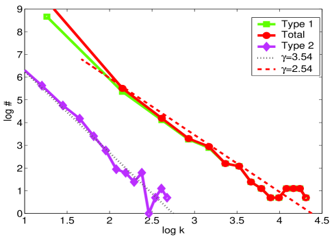
Figure 1: An example of a grown heterogeneous network with multiple scale-free structures: The network comprises two classes of nodes, and nodes in both classes follow the same overall preferential dynamics: when joining the network, every node selects target nodes preferentially until a total of $m$ preferential connections are made. The only deviation from the well-known preferential dynamics is that if a preferentially chosen node refuses a connection request, then the requesting node makes another independent preferential selection and repeats the process until a request is accepted. The dynamical rule differentiating the two classes is that while Type-1 nodes always accept all the connection requests ($d_{1}=1$), Type-2 nodes randomly accept only half the requests ($d_{2}=0.5$). The two classes have equal representation, i.e., $s_{1}=s_{2}=0.5$. As shown in the degree distribution plots, this dynamic leads to two distinct scaling features: A heavy-tailed degree distribution, $\gamma_{1}\sim 2.54$, for Type-1 (squares), and a light-tailed distribution, $\gamma_{2}\sim 3.54$, for Type-2. Interestingly, the overall degree distribution (circles) closely resembles the degree distribution of Type-1 nodes, and hence, if the nodes are not differentiated then the whole network will be characterized by a single scaling parameter, $\gamma\approx 2.54$. In general, single scaling parameter characterizations of heterogeneous networks will always hide the structure of all the classes of nodes, except that of the most heavy-tailed one: Consider the case of a network consisting of two classes of nodes, $A$ and $B$, with PL exponents $\gamma_{A}$ and $\gamma_{B}$, respectively. If $\gamma_{A}<\gamma_{B}$ then the overall degree distribution is thus $P(k)\sim k^{-\gamma_{A}}+k^{-\gamma_{B}}\sim k^{-\gamma_{A}}$ when $k\gg 1$.

Does the presence of an exponent $\gamma<3$ mean that one of the alternate mechanisms is at work? As illustrated in Fig. 1, the presence of a heavy-tailed degree distribution need not necessarily imply that the simple linear preferential attachment is not at play. Indeed, a PL degree distribution with exponent less than $3$ can result from the standard linear preferential attachment dynamic if the network, for example, has two classes of nodes with varying acceptance or attachment rates. In this example, a node joining a network still makes globally preferential links, except that when the request reaches one of the classes, it rejects it with probability $1/2$ while the other class always accepts a connection for request. From a mechanism perspective, if one did not view this as a heterogeneous network, then one might be misled to infer that the underlying dynamic was something other than the standard preferential attachment.

I.5 Implications: Designer Complex Networks

In terms of explicitly designing heterogeneous dynamic networks, an example of great practical interest is the class of ad-hoc distributed systems, with peer-to-peer (P2P) content-sharing networks as a prime example. As discussed in more detail in Section VI, a P2P network has heterogeneous sets of nodes with varying lifetimes and bandwidth capabilities. A natural question is how to design local dynamics such that an overall scale-free structure will emerge, where each node category has a distribution that suits its available resources and needs. We add an additional stringent design constraint: A node joining the network has no global knowledge of which nodes belong to which category, and it can only explore the network locally and only request connections to nodes that it can reach. The dynamics introduced in this paper provide a systematic solution to this challenging problem.

The primary motivations for designing local dynamics so that a PL topology emerges include, (i) PL networks are resistant to random deletions and have vanishingly small percolation thresholds zerothresh ; (ii) PL networks have a natural hierarchy allowing more capable processors to act as hubs; moreover, computing resources are heterogeneous to begin with and PL networks provide a natural set-up for the resource hierarchy to be embedded into a networking hierarchy, and (iii) the structure of PL networks can be exploited to provide scalable key-words based search capabilities perc ; p2p ; tcs . While these properties of PL networks, have been proven to be true for random PL networks, our recent results show that the grown random networks generated using the local dynamics formulated in this paper (particularly, the ad hoc dynamics, where nodes randomly leave the network) lead to networks that are much closer to random PL graphs than those generated by previously-proposed algorithms Callaway01 unpublished-us .

I.6 Prior Work

Previously known dynamical models have mainly characterized the scale-free structure of the emergent networks with a single state (manifested by the overall power-law exponent). Nonuniform preference kernels and their effect on the overall power-law exponent of the emerging network has bee considered before in the context of fitness models. In fitness , a node dependent preferential attachment kernel is introduced. As a new node $i$ enters the network, it is assigned a fitness factor $\eta_{i}$ randomly drawn from some distribution. The probability of the node $i$ receiving a new connection when its current degree is $k_{i}$ will be proportional to $\eta_{i}k_{i}$.

The argument is that different nodes in the network can have different inherent attractions. As such, a new node with a high fitness can gain more connections over time compared to an old node with a smaller fitness. This can explain, for instance, the high connectivity of some new pages in the WWW. The authors then derive the overall degree distribution as a function of the distribution of the $\eta_{i}$’s. The same multiplicative fitness mode is adopted in dog-fitness for the case of directed preferentially grown graphs. In particular, it is shown that even a single node with a high fitness can acquire almost all the links in the network over time, corresponding to a condensation to a star-like topology. The work of dog-fitness also considers the case of the mixture of two ”weak” and ”strong” classes which closely relates to the model considered in this paper when $Q=2$ and $c=0$. However, a detailed study of the emergence of different scale-free structures in heterogeneous networks, and their dependencies on dynamical parameters have not been addressed prior to this work.

I.7 Organization of the paper

The rest of the paper is organized as follows. In Section II, we describe a dynamical model of the networks considered in this paper. We formally introduce the four parameters that can be used to characterize the different categories of nodes. In general, all four of these parameters could be non-uniform over the classes of nodes in the network. However, for the sake of analysis and also understanding the roles of different dynamics in determining emergence of scale-free structures, we study cases where only one or two of these parameters are nonuniform over the nodes in the network, and the others are held uniform. For example, in Section III we first analyze the model by considering the effects of only attractions and representations, as these parameters are varied for different classes of nodes. Moreover, we consider a dynamic ad hoc network, where nodes both join and leave the network. Next in Section IV, we solve the model for the case of uniform attractions, but heterogeneous stability, responsiveness, and representation properties. We are interested in explicitly tracking the structure of each subclass and investigating the fundamental constraints that the intra-class interactions of a particular class will impose on its emerging structure. To our particular interest is the coexistence of different phases in different classes. In Section V we explicitly address this issue and look at the structure of the phase space, and phase transitions that occur. In particular, we are interested in the heavy and light tailed degree distributions of subnetworks. Concluding remarks and applications of the dynamic rules investigated in this paper to the design of P2P networks are provided in Section VI.

II Model Parameters

A list of the parameters and variables used in this paper, along with their definitions, can be found in Table 1. Throughout this paper, $q\in\{1,2,...,Q\}$ will represent the type or class or category (all three terms are used interchangeably) of a node in a network in which nodes can belong to one of $Q$ different classes.

The dynamics for network evolution considered in this paper can be summarized as follows:
(i) Addition of Nodes: At each time step, a new node is introduced into the network, the new node can belong to any of the $Q$ different classes or types indexed by an integer $q=1,2,...,Q$. The probability of the new node being of type $q$ is assumed to be $s_{q}$, where $\displaystyle\sum_{q}s_{q}=1$.
(ii) Creation of Links: The new node, inserted at time step $t$, then makes $m$ connections by picking nodes preferentially using the well known linear kernel. Target nodes, however, can refuse requests for connections, and hence, the new node performs the following procedure $m$ times: It chooses a node preferentially; thus the probability of choosing a node $i$ in the $q^{th}$ class is $\displaystyle\frac{k(i,t;q)}{\sum_{j,p}k(j,t;p)}$ where $k(i,t;q)$ is the degree of the $i^{th}$ node in class $q$, at time step $t$ (see Table 1). The new node then sends a connection request to this selected candidate. The candidate node $i$ will accept the connection with probability $d_{q}$ depending on its type $q$. If the connection is refused then, the new node has to repeat the process until it finds a node that accepts a new connection.
(iii) Deletion of Nodes: At each time step, for each class $q=1,2,...,Q$ a randomly selected node of type $q$ and all its links are deleted with probability $c_{q}$. Thus, the total deletion rate is $c=\sum_{i=1}^{Q}c_{q}<1$.
(iv) Compensation for Lost Edges: If a node looses a link due to deletion of one of its neighbors, a node of type $q$ will introduce $n_{q}$ new links following the same linear preferential procedure outlined above in step (ii).

An important characteristic of this model is that it is local and private in the sense that only a node itself, and not the other members including the nodes trying to connect to it, has any knowledge about its type.

The parameters $s_{q},d_{q},c_{q}$, and $n_{q}$ thus represent the heterogeneity in the population, attraction/attachment, stability and responsiveness dynamics that characterize the different categories of nodes:

II.1 Nonuniform Attraction ($d_{q}$)

Different categories of nodes might have different degrees of attraction (also known as fitness in d3 ) that can influence the structure of all the classes. That is, a class of nodes might be more willing to accept the requests for new connections than the others.

II.2 Nonuniform Stability ($c_{q}$)

The degree of stability of the nodes in different classes might be different. In an ad-hoc network, where nodes can join and leave the network, some classes of nodes might be inherently more stable than others. Those classes, by the virtue of the fact that they would stay longer periods of time in the network, will tend to acquire larger fractions of the connections and usually tend to become more heavy-tailed. The interaction of the classes of ”older” nodes and the class of ”fresh” nodes is fairly interesting. The phases of the subnetworks can be tracked separately for instance to determine the situations in which the subnetwork of ”old” nodes will acquire almost all the links of the network.

II.3 Nonuniform Responsiveness ($n_{q}$)

The degree of responsiveness of different sets of nodes to changes in the network might be different. We examine the effects of heterogenous compensation magnitudes for the lost links. In a compensation mechanism as introduced in us , a node will react to losing a neighbor by initiating a number of new connections to compensate for its lost links. The number of such compensatory connections is an indication of the degree with which the node responds to its changes. We show that the different degrees of responsiveness in different classes will influence the structure of other classes and the overall network.

II.4 Nonuniform Population Size ($s_{q}$ and $c_{q}$)

As stated in Table 1, the number of nodes of type $q$ at time $t$ in the network is given by $N(t;q)=(s_{q}-c_{q})t$. Hence, by varying $s_{q}$ and $c_{q}$ the proportions of different classes of nodes can be varied. In the special case of two classes one can define a majority and a minority class, and then study the effect of the relative populations of the different classes on the PL exponent of the degree distributions of each class. We derive in Sections III and IV, the role that sizes of the majority and minority classes play in determining the overall network structure.

Table 1: Nomenclature

Variable	Definition	Relation
$Q\quad$	the number of different types of nodes
$q\in\{1,2,...,Q\}\quad$	denotes a particular class
$m\quad$	number of links per newly inserted node
$s_{q}\quad$	is the fraction of nodes of type $q$, per newly inserted	$\sum_{q}s_{q}=1$
$c\quad$	the fraction of nodes deleted per an inserted node
$c_{q}\quad$	the fraction of nodes of type $q$ deleted per an inserted node	$\sum_{q}c_{q}=c$
$d_{q}\quad$	the probability that a node of type $q$ accepts a request for connection.
$m_{q}$	the probability of requesting a node of class $q$ for connection	$m_{q}=L(t;q)/L(t)$
$\delta_{q}\quad$	the probability of a new link to be finally connected to a node of class $q$	$\delta_{q}=\frac{m_{q}d_{q}}{\sum_{p=1}^{Q}(m_{p}d_{p})}$ .
$L(t;q)\quad$	the sum of the degree of all nodes of type $q$ ($\sum_{i}k(i,t;q)$).
$L(t)\quad$	the sum of the degree of all nodes in the network (twice the number of all links)	$L(t)=\sum_{q}L(t;q)$
$k(i,t;q)\quad$	the degree of a node $i$ of type $q$ at time step $t$.
$D(i,t;q)\quad$	the probability that a node of type $q$ inserted at time $i$ is still in the network at time $t$.	$D(i,t;q)=(\frac{t}{i})^{-\frac{c_{q}}{s_{q}-c_{q}}}$
$\gamma_{q}\quad$	the power-law exponent of the scale-free degree distribution in class $q$ ($p_{q}(k)\propto k^{-\kappa}$).

III Nonuniform Attraction and Population

We consider the case where the different classes are characterized by different values of $d_{q}$ (acceptance probability) and $s_{q}$ (population size). We assume that there is no compensation, i.e., $n_{1}=n_{2}=\cdots=n_{Q}=0$, and that the deletions of nodes are made uniformly over all the classes, i.e., $c_{q}=c*s_{q}$. Note that the homogeneous case, where there is only one class, i.e., $|Q|=1$, was solved in us . Let $i_{t;q}$ be the set of all nodes of type $q$ that are present in the network at time $t$. When a new link chooses a node $i\in i_{t;q}$ for connection, $i$ can accept to attach to it with some probability $d_{q}$ and deny the attachment with probability $1-d_{q}$. Once denied, the new link will have to repeat the process to choose another target node for connection.

We first provide the following reduction: the protocol for selecting target nodes globally preferentially, until a node is found that accepts the connection, is equivalent to first selecting a class $q$ with probability $\delta_{q}$, and then making a connection to the $i^{th}$ node in the class with probability proportional to its degree as normalized with respect to the sum of the degrees of all nodes only in the $q^{th}$ class, i.e., the probability that the $i^{th}$ node in class $q$ will receive an edge is $\displaystyle\frac{\delta_{q}k(i,t;q)}{L(t;q)}$, where $L(t;q)$ is the sum of the degrees of nodes in class $q$ (see Table 1). In the equivalent protocol, the process of acceptance and denial is captured by the parameter, $\delta_{q}=f(d_{q},s_{q})$, which is the steady state probability of the new link being finally connected to a node of type $q$; the relationship among $\delta_{q},d_{q},s_{q}$ is derived later in this section. The modified protocol is derived to make our analysis simpler.

Next we prove the equivalence of the modified protocol (where the incoming node needs to select a class first, and hence, require global knowledge) to the original protocol (where the incoming node has no knowledge of the different class). Let (i)$A_{q}$ be the event that a node of type $q$ is the end node of a successful link attempt; hence, $p(A_{q})=\frac{L(t;q)}{L(t)}=m_{q}$, (ii) $C_{i;q}$ be the event that a node $i$ of type $q$ is requested for a connection. Then, $p(\hbox{a new link is established}|C_{i;q})=d_{q}$, and $p(C_{i;q})=\frac{k(i,t;q)}{L(t)}$. Also, $p(\hbox{a new link is established })=\sum_{p=1}^{Q}m_{p}d_{p}$, and we are interested in $p(C_{i;q}|\hbox{a new link is made})$. Using Bayes’ rule, we get:

$$p(C_{i;q}|\hbox{ a new link is made})$$ (1)

$$= \frac{p(\hbox{ a new link is established}|C_{i;q})p(C_{i;q})}{p(\hbox{ a new link is established })}$$

$$= \frac{d_{q}k(i,t;q)}{L(t)(\sum_{p=1}^{Q}m_{p}d_{p})}$$

$$= \frac{d_{q}m_{q}}{\sum_{p=1}^{Q}m_{p}d_{p}}\frac{k(i,t;q)}{L(t;q)}$$

$$= \delta_{q}\frac{k(i,t;q)}{L(t;q)}\ .$$

The expressions for $L(t;q)$ and $m_{q}$ are derived later in this section.

The continuous rate equation approach Dog3 ; us can now be employed to track $k(i,t;q)$, at a time $t\geq i$ in the equivalent protocol:

$$\frac{\partial k(i,t;q)}{\partial t}=\frac{m\delta_{q}k(i,t;q)}{L(t;q)}-c\frac{k(i,t;q)}{N(t)},$$ (2)

where (i) the first term represents the fraction of new links that the $i^{th}$ node of type $q$ gets due to the addition of $m$ new links at each step (see Eq. (1)), and (ii) the second term represents the fraction of edges lost due to the deletion of a randomly picked node at each time step. Note that, in general $N(t;q)=(s_{q}-c_{q})t$, and since in the case of uniform deletion $c_{q}=c*s_{q}$, we get $N(t;q)=s_{q}(1-c)t$. Similarly, a rate equation for $L(t;q)$ can be written as:

$$\frac{\partial L(t;q)}{\partial t}$$

$$= m(\delta_{q}+s_{q})-cL(t;q)/N(t)-c\frac{L(t;q)}{L(t)}\frac{L(t)}{N(t)}$$

$$= m(\delta_{q}+s_{q})-L(t;q)\frac{2c}{(1-c)t},$$

where (i) the first term in Eq. (III) captures the following dynamic: A new node brings $m$ links to the network. With probability $s_{q}$ this new node is of type $q$ and with probability $\delta_{q}$ one of its ends will be connected to a node of type $q$; (ii) The second term in Eq. (III) captures the following dynamic: When a node is deleted, it might be of type $q$ with probability $N(t;q)/N(t)$, and the class $q$ will lose an average of $L(t;q)/N(q,t)$ links, resulting in an average contribution to $L(t;q)$ of $-c(N(t;q)/N(t))\times L(t;q)/N(t;q)=-cL(t;q)/N(t)$; and (iii) the third term in Eq. (III) corresponds to the links that nodes of class $q$ lose due to their neighbors being deleted: When a node is deleted, an average number of $L(t)/N(t)$ edges are deleted; now the fraction of these edges that are connected to nodes of type $q$ is $L(t;q)/L(t)$.

$L(t;q)$ is then found to be:

$$L(t;q)=m(\delta_{q}+s_{q})\frac{1-c}{1+c}t\ .$$ (4)

Inserting it back into (2) we get,

$$\frac{\partial k(i,t;q)}{\partial t} = \frac{\delta_{q}k(i,t;q)(1+c)}{(\delta_{q}+s_{q})(1-c)}-c\frac{k(i,t;q)}{(1-c)t}$$

$$= \frac{(\delta_{q}-cs_{q})k(i,t;q)}{(\delta_{q}+s_{q})(1-c)t},$$

which implies $k(i,t;q)=m(t/i)^{\beta_{q}}$, for:

$$\beta_{q}=(\delta_{q}-cs_{q})/[(1-c)(\delta_{q}+s_{q})].$$

Next, using the relationship $(\gamma-1)\beta=1/(1-c)$ developed in us we get

$$\gamma_{q}-1=\frac{(\delta_{q}+s_{q})}{\delta_{q}-cs_{q}}.$$ (5)

At this point, we can make several observations about the coexistence of different phases for the different classes of nodes and the achievability of different exponents for the different classes by varying the attraction rates.

III.1 Tuning exponents $\gamma_{q}$’s and attraction probabilities $d_{q}$’s

Recall that in Eq. (1) we derived the following relationship:

$$\delta_{q}=\frac{m_{q}d_{q}}{\sum_{p=1}^{Q}m_{p}d_{p}},$$ (6)

where $m_{q}=L(t;q)/L(t)$. Note that $L(t)=\sum_{q}L(t;q)$ $=mt(1-c)/(1+c)$, and hence using the result of Eq. (4), we get $m_{q}=L(t;q)/L(t)=(\delta_{q}+s_{q})$, which gives:

$$\delta_{q}=\frac{d_{q}(\delta_{q}+s_{q})}{\sum_{q^{\prime}}(\delta_{q^{\prime}}+s_{q^{\prime}})d_{q^{\prime}}}$$ (7)

Given $d_{q},s_{q},$ for $q=1,2,...,Q$, (7) defines $Q$ equations which can be solved for the $Q$ unknowns $\delta_{q}$. Thus, without loss of generality, we may assume that $\delta_{q}$’s are known and unique for any given set of $d_{q}$’s and $s_{q}$’s. Hence, we can uniquely find $\gamma_{q}$’s, for a fixed set of $d_{q}$’s, $s_{q}$’s and $c$.

Conversely, for a fixed set of $\delta_{q}$’s and $s_{q}$’s, the set of equations in (7) is linear in $d_{q}$ (multiplying by the denumerator of the right hand side) . Arbitrarily normalizing $d_{q}$’s to define a new set of variables $d^{\prime}_{q}=d_{q}/d_{1}$, $d^{\prime}_{q}$’s can be found by solving the following linear system of $Q-1$ equations:

$$\sum_{q^{\prime}=1}^{Q}d^{\prime}_{q}(\delta_{q^{\prime}}+s_{q^{\prime}})(\delta^{\prime}_{q}-I_{q;q^{\prime}})=0$$

for $q=2,3,...,Q$ and setting $d^{\prime}_{1}=1$. The above system of equations is easily shown to be non-singular if and only if $\delta_{q}+s_{q}>0$ for all $q=1,2,...,Q$. In fact the determinant of the system of equations is easily shown to be $\prod_{q=2}^{Q}(\delta_{q}+s_{q})$. This shows the existence of attraction probabilities $d_{q}$ such that any set of power-law exponents as constrained by Eqs. (5) and (III) can be achieved.

III.2 Co-dependencies of the feasible PL exponents for different classes

As discussed above, by sweeping over the parameters $s_{q}$’s and $d_{q}$’s one can effect a continuum of power-law exponents $\gamma_{q}$’s, as determined by Eqs. (5) and (7). The set of possible $\gamma_{q}$’s are however coupled through the requirement that $\sum_{q}\delta_{q}=\sum_{q}s_{q}=1$. As an example, one can define two average quantities involving the power-law exponents:

$$E_{node}(\gamma)=\sum_{q=1}^{Q}s_{q}\gamma_{Q}\hbox{ and }E_{link}(\gamma)=\sum_{q=1}^{Q}2^{-1}(\delta_{q}+s_{q})\gamma_{q}\ \ ,$$ (8)

where $E_{node}$ captures the fact that the averaging is taken over randomly chosen nodes (i.e., probability that the class of a randomly chosen node has exponent $\gamma_{q}$ is $s_{q}$), and $E_{link}$ captures the fact that the averaging is done over random endpoints of a randomly chosen edge, i.e., the probability that a random endpoint of a randomly chosen edge belongs to the $q^{th}$ class is $(\delta_{q}+s_{q})/2$. Now it follows from Eq. (5) that

$$E_{link}((\gamma-1)^{-1})=\sum_{q=1}^{Q}2^{-1}(\delta_{q}+s_{q})(\gamma_{q}-1)^{-1}=(1-c)/2\ .$$ (9)

For the special case of no deletion ($c=0$) it follows from (5) that:

$$E_{node}((\gamma-2)^{-1})=\sum_{q=1}^{Q}(\gamma_{q}-2)^{-1}s_{q}=1$$

The convexity of the function $f(x)=1/x$ :

$$E_{nodes}\{(\gamma-2)^{-1}\}\geq(E_{nodes}\{\gamma\}-2)^{-1}=1$$

or $E_{nodes}\{\gamma\}\geq 3$. In other words, on average the communities of the nodes have power-law exponents greater than 3. On the other hand, this also implies that even for the simple preferential attachment, heterogeneity can lead to an overall degree distribution with exponent $<3$.

When $Q=2$, the two exponents $\gamma_{1}(d_{1},d_{2}),\gamma_{2}(d_{1},d_{2})$ can be explicitly found as functions of $d_{1},d_{2}$. By eliminating $d_{1},d_{2}$, the set of possible power-law exponent pairs $(\gamma_{1},\gamma_{2})$ can be derived. An example of this is depicted in Fig. 2 for $s_{1}=0.8,s_{2}=0.2$ for different values of $c$. To interpret the asymptotes, first note that from (5), stable network operation is only possible when $\delta_{q}>cs_{q}$, otherwise the class $q$ will become extinct (i.e., will loose all its links). Take class $1$ for instance. Since $\delta_{2}>cs_{2}$, then $\delta_{1}=1-\delta_{2}<1-cs_{2}=1-c+cs_{1}$, which results in: $\gamma_{1}\geq 1+(1-c+cs_{1}+s_{1})/(1-cs_{2}-cs_{1})=2+s_{1}(1+c)/(1-c)$. The same bound can be found for class $2$ as well. Some of these asymptotes are also depicted in Fig. 2.

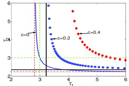
Figure 2: Possible power-law exponents in a network with two classes of nodes. $\gamma_{1}$ is the power-law exponent of the degree distribution of the first class that consists of $80\%$ of all nodes, while $\gamma_{2}$ correspond to the second class consisting of $20\%$ of all nodes. The possible power-law exponents for three deletion rates $c=0,0.2,0.4$. The asymptotes for $c=0$ and $c=0.2$ are also depicted.

III.3 Role of deletion rate $c$

It was shown in us that when $|Q|=1$, i.e., there is only one class and the network is homogeneous, then $\gamma$ is always greater than 3 for any deletion rate $c>0$. Moreover, even for small values of $c$ the exponent becomes quite large, and the network shows none of the characteristics associated with heavy-tailed PL degree distributions. In the case of heterogeneous networks, however, one can have a class with a true heavy-tailed degree distribution (as illustrated in Figs. 2 and ), and the overall network will thus exhibit a heavy-tailed distribution, even for non-zero deletion rate $c$. However, as $c\rightarrow 1$, we get (see Eqn. 9): $\sum_{q}(\delta_{q}+s_{q})(\gamma_{q}-1)^{-1}=0$. Thus, in the limit of heavy node deletion, the degree distribution of any class $q$ with a finite size ($s_{q}>0$) becomes exponential (i.e., $\gamma_{q}\rightarrow\infty$ for all $q=1,...,Q$).

In the next section, a compensatory mechanism is examined, which will result in classes with prescribed heavy or light tailed degree distributions, even in the limit of very high deletion rates. Moreover, while the deletion process in this section was independent of the class of nodes (a node was randomly chosen for deletion), in practice, different classes of nodes will have different stability characteristics. This important generalization is made in the following section.

IV Heterogenous Stability and Responsiveness

Many ad-hoc networks are characterized by the fact that the time scale within which their size grows, is much larger than the time scale within which the nodes join and leave the network. In such networks (certainly including P2P file sharing systems) one has the case that $c\approx 1$. The scale free properties of growing networks that are subject to permanent deletion of their nodes are studied in Dog3 ; us . In us , the heavy-tailed structure of the resulting scale-free networks were shown to immediately disappear in the presence of node deletion. Results in the previous section also showed that no heavy tailed structure can exist in the limit of high deletion rates even in a heterogenous network.

A universal compensatory protocol has been introduced by the authors in us , which ensures that the heavy tail of the degree distribution of the emerging network is conserved even in the limit of very high node departure rates. This section will investigate the behavior of different classes of a network of multiple types in the presence of (i) heterogenous node deletion or equivalently, heterogeneous stability factors, and (ii) heterogeneous responsiveness, i.e., the rate at which different classes of nodes compensate for their lost or dead links is class dependent. A class dependent compensatory mechanism is a generalization of the universal compensation scheme in us , and it plays a crucial role in restoring the heavy-tailed structure of some or all of the classes in the network.

The dynamical model introduced in Section II allows for non-uniform deletion of nodes and compensation of links. For simplicity we would assume uniform attraction, i.e., $d_{1}=d_{2}=...=d_{Q}=1$, that is, all nodes accept all requests for connections. We let the other parameters $s_{q},n_{q},c_{q}$ be arbitrary. The goal is to characterize the emerging scale free state of each of the $Q$ sub-networks as a function of these dynamical parameters.

IV.1 Rate Equation Formulation

A mean-field rate of change of $k(i,t;q)$ can be written as:

$$\frac{\partial k(i,t;q)}{\partial t}=\frac{mk(i,t;q)}{L(t)}-c(1-n_{q})\frac{k(i,t;q)}{N(t)}$$

$$+ \frac{k(i,t;q)}{L(t)}\left(\sum_{q^{\prime}}n_{q^{\prime}}\frac{L(t;q^{\prime})}{L(t)}\right)\left(\sum_{q^{\prime\prime}}c_{q^{\prime\prime}}\frac{L(t;q^{\prime\prime})}{N(t;q^{\prime\prime})}\right)$$

where, (i) the first term comes from the contribution of the $m$ new links inserted at time step $t$ when $L(t)$ is the sum of the degree of all nodes of type $q$ (remember that we assume uniform preferential attachment). (ii) The second term captures the effect of the random deletion of one of the neighbors of $i$ which is compensated with $n_{q}$ preferentially targeted new links (hence the $1-n_{q}$ multiplier). (iii) The third term is due to the attraction of the compensatory links from other nodes rather than $i$. It assumes that an average of $\left(\sum_{q^{\prime\prime}}c_{q^{\prime\prime}}\frac{L(t;q^{\prime\prime})}{N(t;q^{\prime\prime})}\right)$ links are deleted, of which a fraction of $\frac{L(t;q^{\prime})}{L(t)}$ belongs to a particular class $q^{\prime}$ and will be compensated by $n_{q}^{\prime}$ preferentially targeted new links.

To find $L(t;q)$, its rate of change can be tracked as below:

$$\frac{\partial L(t;q)}{\partial t} =$$

$$= ms_{q}+m\frac{L(t;q)}{L(t)}-c_{q}(1-n_{q})\frac{L(t;q)}{N(t;q)}$$

$$- \frac{L(t;q)}{L(t)}\left(\sum_{q^{\prime}}c_{q^{\prime}}\frac{L(t;q^{\prime})}{N(t;q^{\prime})}\right)$$

$$\times \left(1-\sum_{q^{\prime\prime}}n_{q^{\prime\prime}}\frac{L(t;q^{\prime\prime})}{L(t)}\right)$$

where (i) the first terms corresponds to the new links added to the class $q$ if the new node happens to be of type $q$ (this occurs with probability $s_{q}$), (ii) the second terms is due to the end of new links being connected to a node of type $q$. (iii) The third term comes from the deletion of an average of $L(t;q)/N(t;q)$ links if a node of type $q$ is deleted, which is compensated by $n_{q}$ new links per lost link. (iv) The forth term is similar to the third term in (IV.1). In the steady state one has $L(t;q)\approx B_{q}t,N(t;q)=(s_{q}-c_{q})t,N(t)=(1-c)t$. The $Q$ unknowns $B_{q}$ can thus be found through the following set of $Q$ equations (one for each $q=1,2,...,Q$):

$$B_{q} =$$

$$= m\left(s_{q}+\frac{B_{q}}{\sum_{q^{\prime}}B_{q^{\prime}}}\right)$$

$$- \frac{c_{q}}{s_{q}-c_{q}}(1-n_{q})B_{q}$$

$$- \frac{B_{q}}{\sum_{q^{\prime}}B_{q^{\prime}}}\left(1-\sum_{q^{\prime\prime}}n_{q^{\prime\prime}}\frac{B_{q^{\prime\prime}}}{\sum_{q^{\prime}}B_{q^{\prime}}}\right)\left(\sum_{q^{\prime\prime}}\frac{c_{q^{\prime\prime}}}{s_{q^{\prime\prime}}-c_{q^{\prime\prime}}}B_{q^{\prime\prime}}\right)$$

Finding $B_{q}$’s and inserting back into (IV.1), $k(i,t;q)$ is found to be:

$$k(i,t;q) = m(t/i)^{\beta_{q}}$$ (12)

for $\beta_{q}$ a function of $B_{q},c_{q},s_{q},n_{q}$’s as below:

$$\beta_{q}=\frac{m}{B}-\frac{c(1-n_{q})}{s_{q}-c_{q}}+\frac{\sum_{q^{\prime}}n_{q^{\prime}}B_{q^{\prime}}}{B}\times\sum_{q^{\prime\prime}}\frac{c_{q^{\prime\prime}}B_{q^{\prime\prime}}}{s_{q}-c_{q}}$$ (13)

where $B=\sum_{q}B_{q}$.

Now define $D(i,t;q)$ the probability that a node of type $q$, inserted at time $i$ is still in the network at time $t$. $D(i,t;q)$ can be found as follows:

$$\frac{\partial D(i,t;q)}{\partial t} = -c_{q}D(i,t;q)/N(t;q)$$

$$= -c_{q}D(i,t;q)/[(s_{q}-c_{q})t]$$

resulting in, $D(i,t;q)=(t/i)^{-c_{q}/(s_{q}-c_{q})}$.

Finally, $P_{q}(k)$, the degree distribution of the nodes of type $q$ can be found as follows:

$$P_{q}(k) = \frac{\hbox{No. of nodes of type $q$ with degree $=\ k$}}{\hbox{Total number of nodes of type $q$}}$$ (14)

$$= \frac{1}{N(t;q)}\sum_{i:k(i,t;q)=k}N(t;q)D(i,t;q)$$

$$= \displaystyle D(i,t;q)\left|\frac{\partial k(i,t;q)}{\partial i}\right|_{i:k(i,t;q)=k}^{-1}$$

Solving for $i$, such that $k(i,t;q)=k$ from (12), and inserting back into (14) we arrive at:

$$P_{q}(k)\propto k^{-c_{q}/[(s_{q}-c_{q})\beta_{q}]-1/\beta_{q}-1}\propto k^{-\gamma_{q}}$$

from which the power-law exponents are found to be:

$$\gamma_{q} = 1+\frac{s_{q}}{\beta_{q}(s_{q}-c_{q})}$$

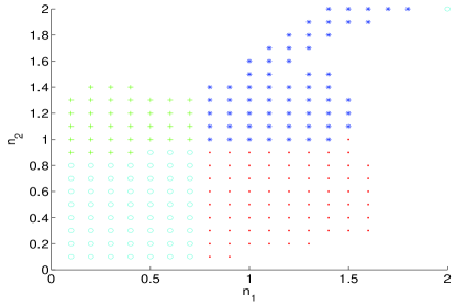
Figure 3: Different regions of the power-law exponents for an example consisting of two classes of nodes with $s_{1}=0.8,s_{2}=0.2,c_{1}=0.6,c_{2}=0.15$ for various compensation magnitudes $0<n_{1},n_{2}<2$. (i) The circles indicate the region in which class one is light tailed while class two is heavy tailed. (ii) Squares indicate the phase where both classes are heavy tailed (iii) both classes are light tailed where indicated by diamonds and (iv) asterixes indicate that the first class is heavy tailed while the second class is light tailed.

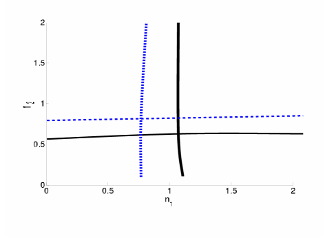
Figure 4: Phase diagram of a mixture of two classes of nodes. The entry rate of the two classes are the same $s_{1}=s_{2}=0.5$. The axes correspond to $n_{1},n_{2}$. The curves represent the points in $(n_{1},n_{2})$ for which either $\gamma_{1}=3$ or $\gamma_{2}=3$. The dashed curves are for the case of $c_{1}=c_{2}=0.3$ and are hence symmetric. As the deletion rates becomes un-balances, the phases curves also shift. The solid curves correspond to the deletion rates $c_{1}=0.4,c_{2}=0.3$. It therefore takes more compensation for the first class to retain its heavy tail. Now the second class in its turn will acquire some of these excess compensations. Thus, overall the class two will need less compensation to stay heavy tailed. The net result is a shift of the phase diagram to the south-east.

Finding the set of $\gamma_{q}$’s requires the tedious task of solving the system of equations (IV.1) to find $B_{q}$’s and then plugging the $B_{q}$’s back into (13) to get the $\beta_{q}$’s and finally finding $\gamma_{q}$’s through (IV.1). Such procedures are carried out for a number of examples in the next section.

V Phase Diagrams and Topological Observations

V.1 Phase Diagrams

There are four particularly interesting emergent phases for a subclass of nodes of a network:

• The Light-Tailed phase, in which the network emerges into a quasi-equilibrium state in which the average degree of the nodes is bounded and non-zero, and the variance of the degree distribution is also bounded.

• The Heavy-Tailed phase, corresponding to a subnetwork with finite average degree but diverging variance of the degree distribution. Such networks possess many attractive properties (at least in their equilibrium form) like constant diameter or zero percolation probability newman .

• Extinction phase, when the average degree of the subnetwork goes to zero and it looses most of its links.

• Unstable or divergent phase, in which the average degree of the subnetwork diverges and the whole network loses its stability.

Previous sections suggest the procedure for calculating the emergent power-law exponent of all the network classes as a function of the model parameter, $n_{q},c_{q},s_{q}$. This in turn can determine the state of all subnetworks of the network. An example of such procedure is carried out for two classes of nodes with $s_{1}=0.8,s_{2}=0.2,c_{1}=0.6,c_{2}=0.15$ for various compensation magnitudes $0<n_{1},n_{2}<2$. Only the heavy-tailed and light-tailed phases are marked and thus there are a total of 4 possible phases for the whole network depicted in Fig. 3.

The contour in the space of parameters for which $\gamma_{q}=3$ is important because it marks the transition of the phase of the network from a stable light-tailed state into a stable heavy-tailed one. An example is depicted in Fig. 4, in the scope of parameters $n_{1},n_{2}$ for fixed $c_{1},c_{2},s_{1},s_{2}$.

To our special practical interest is the case of quasi-uniscale networks, the networks in which most of the nodes belong to a single category and most deletions and insertions happen in the nodes of this category. Call this category, $q=1$. We then define a quasi-uniscale network as one in which $c_{1}\approx c\gg c_{q},s_{1}\approx 1\gg s_{q},s_{1}-c_{1}\gg s_{q}-c_{q},q\neq 1$.

Class $1$ will be called the majority class and the rest of the classes are called minority classes. It then follows that $L(t,1)\approx L(t)$ and $L(t;q)\ll L(t)$ for all $q\neq 1$ which reduces (IV.1) to: $L(t;q)\approx\delta_{q,1}2m(1-c)t/(1+c-2n_{1}c)$, where $\delta_{q;q^{\prime}}$ is the Kronchker’s delta function. Inserting in (13), the $\beta_{q}$’s are found to be:

$$\beta_{q}\approx\frac{(1-c+2c(n_{q}-n_{1}+n_{1}\delta_{q,1}))}{2(1-c)}$$

from which:

$$\gamma_{1}\approx 1+\frac{2}{1-c+2cn_{1}}$$

$$\gamma_{q}\approx 1+\frac{2r_{q}}{1-c+2c(n_{q}-n_{1})},$$

where $r_{q}=\frac{(s_{q}-c_{q})}{s_{q}(1-c)}$, called the robustness factor of the class $q$ is the fraction of nodes of type $q$ that are in the network over the fraction of nodes that enter per newly inserted node. In the limit of very active quasi-uniscale networks ($c\rightarrow 1$), one gets : $\gamma_{1}\approx 1+1/n_{1}$ while $\gamma_{q}\approx 1+\frac{r_{q}}{n_{q}-n_{1}}$ for $q\neq 1$.

An example of the phases for this limiting case is depicted in Fig. 5.

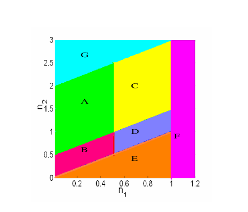
Figure 5: Different phase regions in the space of parameters $(n_{1},n_{2})$, where $n_{1}$ is the compensation rate for the majority class while $n_{2}$ is the corresponding parameter for the minority class. The phases are as follows: (A) The majority is light-tailed while the minority is heavy-tailed. (B) Both the majority and minority are light-tailed (C) Both are heavy-tailed (D) Minority is light-tailed while majority is heavy-tailed (E) The minority extinction (F) Majority becomes unstable (infinite mean) (G) Minority becomes unstable (infinite mean)

Another interesting limit is where only one class compensates for its lost links and the rest of the classes are irresponsive. Consider the case of a mixture of two classes where the first class with $c_{1}=0.8,s_{1}=0.75$ does not compensate ($n_{1}=0$). The phases regions of the second class with $s_{2}=0.25$ are depicted in Fig. 6 as a function of its deletion and compensation rates ($c_{2},n_{2}$).

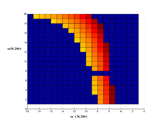
Figure 6: Stable heavy-tailed minority class: The majority class with $s_{1}=0.75,c_{1}=0.8$ is not compensating ($n_{1}=0$). The region in the space of the $n_{2},c_{2}$ where the minority class is stable and heavy tailed (i.e., $2<\gamma_{1}<3$) is highlighted. The part to the left of the region (for higher compensation rates) indicates $\gamma_{1}<2$ while the region to the rights indicates $\gamma_{1}\geq 3$.

V.2 Simulations

For a network of finite size, the variance of the degree distribution is an indication of how heavy-tailed the degree distribution is. Plotting the ratio of the variances at different classes in the space of dynamical parameters will allow us to compare the relative state of different network classes. We have simulated a network of 5000 nodes with two categories of nodes ,$Q=2$, with uniform deletion of magnitude $c=0.5$ and $s_{1}=s_{2}=0.5$ for various compensation magnitudes $n_{1},n_{2}$. We have then plotted the ratio of the variances at each of the classes for each value of $(n_{1},n_{2})$ in Fig. 7.

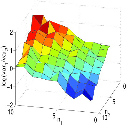
Figure 7: The ratio of the variances of two classes with $c=0.5$, $s_{1}=s_{2}=0.5$ as a function of the compensation magnitudes $n_{1},n_{2}$. The variance of the degree distribution increases as the compensation magnitude of the corresponding class increases.

Simulations to obtain power-law exponents for two classes with equal insertion rates and various deletion rates are depicted in Fig. 8 and verified against the analytical expectations.

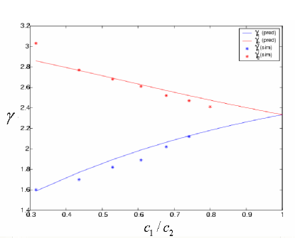
Figure 8: The power-law exponent of a network of two classes with $10000$ nodes. The insertion rates are $s_{1}=s_{2}=0.5$ and the overall deletion rate is a constant $c=0.5$. The deletion rate of the two classes are however different. For various ratios of the deletion rates, the power-law exponent of these two classes are found through simulation. Also depicted are the theoretical predictions of the previous section.

V.3 Topological Observations

As suggested in the introduction, the class of nodes that are more heavy tailed are expected to play more central roles in the topology of the network. The light tailed classes on the other hand would be pushed to the edges of the network serving as leaf nodes. This is a very desirable property for many application including P2P communication systems as discussed in more details in the following section. In this section we try to quantify the place of a category of nodes in the network.

The quantity we consider is the so called capacity of each subnetwork. For a node category $q$, the capacity ${\mathcal{C}}_{q}$ is defined as the total number of edges that have both their ends in a node of type $q$, over twice the total degree of all the nodes of type $q$. When ${\mathcal{C}}_{q}=0$, the category $q$ has all its edges to the outside of the category $q$. On the other hand ${\mathcal{C}}_{q}=1$, all the links of the nodes in category $q$ stay within the same category. One can thus assume that a network with small capacity has a leaf role, while a large capacity is an indication of a more compact topological structure. Fig. 9 depicts the capacities of the two categories of a network of two categories as a function of the relative rate of deletion $c_{1}/c_{2}$. The more stable subnetwork will have a larger capacity, which decreases as $c_{1}/c_{2}\rightarrow 1$.

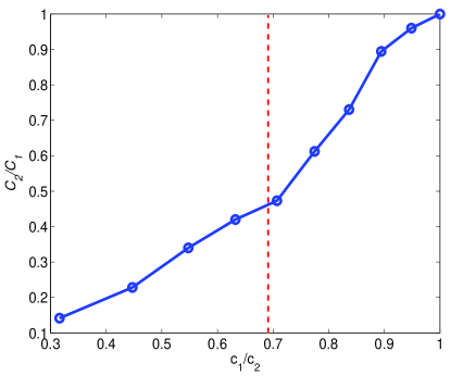
Figure 9: The ratio of the capacities of the two node categories. The network size is 10000, $s_{1}=s_{2}=1/2$ and $c=1/2$. The ratio of the deletion rates for the two categories are varied from 0.3 to 1. The dashed line marks the transition of the first category from a divergent phase into the phase with power-law exponent greater than 2.

VI Concluding Remarks: Applications to P2P Networks

An important example of a complex, highly dynamic, and heterogeneous network (which also partially motivated this research) is the less structured or ad-hoc distributed systems with peer-to-peer (P2P) content sharing networks as a prime example. While nodes in a P2P computer network have heterogeneous resources and lifetimes, they can be classified into a few meaningful classes based on hardware or software characteristics. In particular, the nodes can be categorized into two major classes limewire : (i)Super-nodes with virtually infinite bandwidth (e.g. office users) that run a super-node software and (ii) the low bandwidth home users that run the ordinary software. The fraction of super-nodes is extremely small (around 1% of the whole nodes) but super-nodes are much more stable, with their life times ranging anywhere between 10 to 100 times of the home users.

The integrity of such P2P networks requires most communication paths to be provided by the super-nodes; otherwise, the traffic at the home users will soon exceed their limits and the network structure will be fragmented. This can be ensured only when the network core, that is the highly connected nodes in the network, are mostly super-nodes (or nodes with more capabilities). An ignorance of this fact has led to the apparent break down of the Gnutella network, an early P2P file sharing system in 2000 clip2 .

The dynamics of P2P networks is dominated by the rapid rate of the members joining and leaving the network. More than $60\%$ of all the nodes joining these networks will leave within the first hour, while it takes around three months for the overall size of the network to grow by $60\%$ clip2 . Ensuring the emergence of a heavy tailed scale-free state in such ad-hoc environments is a challenging task. As was shown in Section IV, the same compensatory mechanism developed in us can ensure the emergence of scale-free structures with heavy tails among more stable groups, the groups anticipated to be composed of nodes with high capacity, while the majority of the nodes will have a light tailed degree distribution and are therefore exempted from the search paths. The results of this paper will serve as an essential part of ad-hoc network formation protocols that can support efficient search perc ; p2p ; tcs , robustness, and allow highly dynamic operations.

In passive networks, in which the connections of a new node are never redirected or modified once they are established, the dynamical parameters ($s_{q},n_{q},d_{q},c_{q}$) are usually fixed constants. On the other hand, in most active networks (e.g; P2P applications), some or all of these parameters can be locally manipulated by the nodes. The manipulations of these parameters can be considered as active network design protocols that can modify these parameters and thus can engineer the power-law exponents $\gamma_{q}$. Consider first the possibility of simulated deletion of the nodes of a network. There are classes of networks (e.g. P2P computer networks) in which a node can simulate its departure (log-off) through a software decision. In such networks, the stability of a class of nodes can be manipulated as follows: At each time step, for any $q$, with probability $l_{q}$, a randomly chosen node of type $q$ decides to leave the network (and hence disconnects all its links) and quickly joins back (with $m$ preferentially targeted links). This would then modify the model parameters as follows: $s_{q}\rightarrow(s_{q}+l_{q})/(\sum_{q^{\prime}}l_{q^{\prime}})$, $c_{q}\rightarrow(c_{q}+l_{q})/(1+\sum_{q^{\prime}}l_{q})$. Also, the compensation magnitude $n_{q}$ of any class can be manipulated through the ”software” running on that node. By varying $n_{q}$, the class $q$ can tune its emergent power-law exponent $\gamma_{q}$.

Figure (10) is an example of how the simulated log-off can tune the heavy tailed structure of a class.

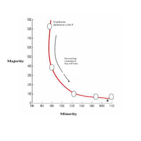
Figure 10: Manipulating Network Structure By Altering Local Rules: The change in the variance of the degree distribution in a network consisting of a majority class ( 90% of the nodes) and a minority class. The network has size 10,000 and both classes compensate with rate $n=1$. At the point indicated by ”uniform deletion”, a uniform deletion with rate $c=0.5$ is in place. The path shows the change in the variance of the degree distribution as the majority starts to simulate a log-off. Without any simulated log-off, the variance in both classes are high, but as the simulated log-off rate increases, the variance of the majority quickly decreases, while the minority remains heavy tailed.

In conclusion, the structure of preferentially grown networks with heterogeneous preference kernels has traditionally been categorized with a single parameter, namely the power-law exponent of the overall scale-free degree distribution of the network, if such scale-free state emerges. We introduced a number of local rules that can tune the emergent scale-free states of different classes and in particular can ensure heavy or light tailed distributions within a particular class. These protocols dealt with four major dynamical elements of the network: The linkage properties of the network; The rate of departure of the nodes in the network; the rate with which nodes of a certain class $q$ compensate for the links they lose; and the rate at which nodes accept requests for connections or links. Different phases of the emergent subclasses under these local rules were characterized and the boundaries of phase transitions were identified.

References

- (1) A.-L. Barabasi and R. Albert, Science 286, 509 (1999).
- (2) A.trusina, S.Maslov, P.Minnhagen and K.Sneppen, ”Hierarchy Measures in Complex Networks,” cond-mat/0308339.
- (3) S.N. Dorogovtsev, J.F.F. Mendes and A. N. Samukhin, Phys. Rev. Lett. 85, 4633 (2000).
- (4) M.E.Newman, Phys. Rev. E., VOL 64, 016131.
- (5) G. Ergun, G. J. Rodgers, ”Growing Random Networks with Fitness”, Physica A 303 (2002) 261-272.
- (6) Ginestra Bianconi and Albert-L szl Barab si Competition and multiscaling in evolving networks Europhysics Letters 54 (4), 436-442 (2001).
- (7) P. L. Krapivsky, S. Redner and F. Leyvraz, Phys. Rev. Lett. 85, 4629 (2000).
- (8) P. L. Krapivsky and S. Redner, Phys. Rev. E 63, 066123 (2001).
- (9) Bianconi,G, A.L. Barabasi, “Topology of evolving networks: local events and universality”, Phys. Rev. Lett. 85, 5234-5237 (2000)
- (10) www.limewire.com
- (11) D. S. Callaway, M. E. J. Newman, , S. H. Strogatz,, and D. J. Watts, ”Network robustness and fragility: Percolation on random graphs”, Phys. Rev. Lett.”, Vol.85, pp 5468-5471, 2000.
- (12) Nima Sarshar and Vwani P. Roychowdhury,Phys. Rev. E 69, 026101 (2004).
- (13) Dorogovtsev, S.N. , Mendes,J.F.F., “Scaling Behaviour of Developing and Decaying Networks”,EuroPhys. Lett. 52, 33 (2000)
- (14) D. S. Callaway, J. E. Hopcroft,, J. M. Kleinberg, M. E. J. Newman, and S. H., ”Are randomly grown graphs really random?”, Phys. Rev. E, Vol. 64, 2001.
- (15) P. L. Krapivsky, G. J. Rodgers, S. Redner“Degree Distributions of Growing Networks,” Phys. Rev. Lett. 86, 5401-5404 (2001)
- (16) Albert,R, A.L.Barabasi “Statistical Mechanics of Complex Networks,”Reviews of Modern Physics 74, 47 (2002)
- (17) William Aiello, Fan Chung, Linyuan Lu, Random evolution in massive graphs IEEE Symposium on Foundations of Computer Science(2001).
- (18) ”The Gnutella Protocol Specification”. Online: http://d ss.clip2.com/GnutellaProtocol04.pdf. 2001
- (19) N.Sarshar, P. O. Boykin, and V.P. Roychowdhury, ”Scalable Percolation Search in Power-Law Networks,” cond-mat/0406152.
- (20) N. Sarshar, P.O. Boykin, V.P. Roychowdhury, ”Percolation Search in Power Law Networks: Making Unstructured Peer-to-Peer Networks Scalable”, IEEE IEEE International Conference on Peer-to-Peer Computing 2004.
- (21) N.Sarshar, P.O. Boykin, V.P. Rychowdhury, ”Scalable Percolation Search on Complex Networks”, submitted to Journal of Theoretical Computer Science, SI: Complex Networks, 2004.
- (22) M.Newman, S.Strogatz and D.Watts, ”Random Graphs with Arbitrary Degree Distributions,” Phys. Rev. E., 64(026118), 2001.
- (23) C. D. Group. Gnutella: To the bandwidth barrier and beyond. Originally found at http://dss.clip2.com/gnutella.html, Nov. 2000
- (24) S.N. Dorogovtsev, J.F.F. Mendes ,Scaling Behaviour of Developing and Decaying Networks, EuroPhys. Lett. 52, 33 (2000).
- (25) G. Bianconi and A.-L. Barabasi, Europhys. Lett. 54, 436 (2001).
- (26) Gnutella: To the Bandwidth Barrier and Beyond,http://dss.clip2.com, Nov. 2000.
- (27) N. Sarshar and V.P. Roychowdhury, ”Percolation properties of Dynamic Networks,” in preperation.