Fractal Structure of High-Temperature Graphs of O($N$) Models in Two Dimensions

Abstract

The critical behavior of the two-dimensional O($N)$ model close to criticality is shown to be encoded in the fractal structure of the high-temperature graphs of the model. Based on Monte Carlo simulations and with the help of percolation theory, De Gennes’ results for polymer rings, corresponding to the limit $N\to 0$, are generalized to random loops for arbitrary $-2\leq N\leq 2$. The loops are studied also close to their tricritical point, known as the $\Theta$ point in the context of polymers, where they collapse. The corresponding fractal dimensions are argued to be in one-to-one correspondence with those at the critical point, leading to an analytic prediction for the magnetic scaling dimension at the O($N)$ tricritical point.

The high-temperature (HT) representation of the critical O($N$) spin model naturally defines a loop gas, corresponding to a diagrammatic expansion of the partition function in terms of closed graphs along the bonds on the underlying lattice Stanley . In the limit $N\to 0$, the loops reduce to closed self-avoiding random walks first considered by de Gennes as a model for polymer rings in good solvents at sufficiently high temperatures, so that the van der Waals attraction between monomers is irrelevant deGennes . In his seminal paper, de Gennes related the fractal structure of self-avoiding random walks to the critical exponents of the O($N\to 0$) model. Invoking concepts from percolation theory and recent Monte Carlo (MC) data geoPotts ; Dotsenko of the HT representation of the two-dimensional (2D) Ising model ($N=1$), we extend in this Letter de Gennes’ result to arbitrary $-2\leq N\leq 2$ in 2D. We consider the loops also close to their tricritical point where they collapse, known as the $\Theta$ point in the context of polymers. We argue that the 2D fractal dimensions at the tricritical point are in one-to-one correspondence with those at the critical point, allowing us to also predict the magnetic scaling dimension at the O($N)$ tricritical point. We support our theoretical prediction by comparing it with recent high-precision MC data bloeteetal .

A particularly simple representation of the O($N$) universality class is specified by the partition function DMNS

$$Z=\mathrm{Tr}\prod_{\langle\mathbf{x},\mathbf{x}^{\prime}\rangle}(1+K\mathbf{S}_{\mathbf{x}}\cdot\mathbf{S}_{\mathbf{x}^{\prime}}),$$ (1)

where the product is over all nearest neighbor pairs, and the spins have $N$ components $\mathbf{S}_{\mathbf{x}}=(S^{1}_{\mathbf{x}},S^{2}_{\mathbf{x}},\dots,S^{N}_{\mathbf{x}})$ and are of fixed length $\mathbf{S}_{\mathbf{x}}^{2}=N$. The trace Tr stands for the sum or integral over all possible spin configurations. The weighting factor is obtained by truncating the more standard Boltzmann weight $\exp(K\mathbf{S}_{\mathbf{x}}\cdot\mathbf{S}_{\mathbf{x}^{\prime}})$. This choice mimics the weighting factor of the Ising model, where $\exp(\beta S_{\mathbf{x}}S_{\mathbf{x}^{\prime}})\propto(1+KS_{\mathbf{x}}S_{\mathbf{x}^{\prime}})$ with $K=\tanh\beta$. When formulated on a honeycomb lattice, which has coordination number $z=3$, the HT graphs of the truncated model are automatically nonintersecting and self-avoiding. The partition function can then be written simply as a sum over all possible closed graphs DMNS , $Z=\sum_{\{G\}}K^{b}N^{l}$, with $b$ and $l$ the number of occupied bonds and separate loops forming the graph $G$. The parameter $K$ in the spin formulation (1) appears as bond fugacity in the loop model. By mapping it onto a solid-on-solid model, the critical exponents as well as the critical point were determined exactly Nienhuis .

In the high-temperature phase, the HT graphs have a finite line tension $\theta_{\mathrm{G}}$ and are exponentially suppressed. A typical graph configuration in this phase shows only a few small loops scattered around the lattice. Upon approaching the critical point from above, the lattice starts to fill up with more and also larger graphs. At the critical point, the line tension vanishes, causing the exponential suppression to disappear. Graphs of all sizes now appear in the system as they can grow without energy cost, i.e., the HT graphs proliferate. A graph spanning the lattice can be found irrespective of the lattice size–much like the appearance of a spanning cluster at the percolation threshold in percolation phenomena StauferAharony . The average number density $\ell_{b}$ of graphs containing $b$ bonds takes asymptotically a form similar to that of clusters in percolation theory,

$$\ell_{b}\sim b^{-\tau_{\mathrm{G}}}{\rm e}^{-\theta_{\mathrm{G}}b},\quad\theta_{\mathrm{G}}\propto(K-K_{\rm c})^{1/\sigma_{\mathrm{G}}},$$ (2)

with $\sigma_{\mathrm{G}}$ and $\tau_{\mathrm{G}}$ two exponents whose values define the universality class. The line tension vanishes upon approaching the critical point at a pace determined by the exponent $\sigma_{\mathrm{G}}$. When present, this Boltzmann factor exponentially suppresses large graphs. The algebraic factor in the graph distribution is an entropy factor, giving a measure of the number of ways a graph of size $b$ can be embedded in the lattice. The configurational entropy is characterized by the exponent $\tau_{\mathrm{G}}$. As in percolation theory StauferAharony , it is related to the fractal dimension $D_{\mathrm{G}}$ of the HT graphs via

$$\tau_{\mathrm{G}}=d/D_{\mathrm{G}}+1,$$ (3)

with $d=2$ the dimension of the lattice.

When summed over all sizes, the graph distribution yields the scaling part of the logarithm of the partition function,

$$\ln Z\sim\sum_{b}\ell_{b}.$$ (4)

Each graph therefore contributes equally to the scaling part of the free energy, irrespective of its size.

Model	$N$	$\bar{\kappa}_{-}$	$c$	$\alpha$	$\beta$	$\gamma$	$\eta$	$\nu$	$D_{\rm G}$	$\tau_{\mathrm{G}}$	$\sigma_{\mathrm{G}}$
Gaussian	$-2$	$\frac{1}{2}$	$-2$	$1$	$0$	$1$	$0$	$\frac{1}{2}$	$\frac{5}{4}$	$\frac{13}{5}$	$\frac{8}{5}$
SAW	$0$	$\frac{2}{3}$	$0$	$\frac{1}{2}$	$\frac{5}{64}$	$\frac{43}{32}$	$\frac{5}{24}$	$\frac{3}{4}$	$\frac{4}{3}$	$\frac{5}{2}$	$1$
Ising	$1$	$\frac{3}{4}$	$\frac{1}{2}$	$0$	$\frac{1}{8}$	$\frac{7}{4}$	$\frac{1}{4}$	$1$	$\frac{11}{8}$	$\frac{27}{11}$	$\frac{8}{11}$
XY	$2$	$1$	$1$	$-\infty$	$\infty$	$\infty$	$\frac{1}{4}$	$\infty$	$\frac{3}{2}$	$\frac{7}{3}$	$0$

Table 1: Critical exponents of the two-dimensional critical O($N$) spin model, with $N=-2,0,1,2$, respectively, together with the parameter $\bar{\kappa}_{-}$ and the central charge $c=1-6(1-\bar{\kappa}_{-})^{2}/\bar{\kappa}_{-}$. In addition, the fractal dimension $D_{\mathrm{G}}$ of the HT graphs as well as the two exponents $\tau_{\mathrm{G}},\sigma_{\mathrm{G}}$ characterizing their distribution are given. For $N=1$, the values of the latter two were recently established numerically in Ref. geoPotts .

Table 1 summarizes the critical exponents and fractal dimensions of the four most common O($N$) models. The negative value $N=-2$ corresponds to the noninteracting model, for which the critical exponents take their Gaussian values BalianToulouse . In the polymer limit $N\to 0$, first studied by de Gennes deGennes , the fractal dimension of the HT graphs is simply the inverse of the correlation length exponent $\nu$. In general, however, it follows from Table 1 that $D_{\mathrm{G}}\neq 1/\nu$. To generalize de Gennes’ result, we note that in percolation theory a similar relation between the fractal dimension $D$ of clusters and the correlation length exponent involves the Fisher exponent $\sigma$, viz. StauferAharony

$$D=1/\sigma\nu.$$ (5)

A closer look at de Gennes’ derivation reveals that $\sigma_{\mathrm{G}}=1$ in that case, implying that the result for polymers in good solvents or self-avoiding random walks is consistent with Eq. (5). In a recent MC study of the HT graphs of the 2D Ising model geoPotts , we numerically found the value $\sigma_{\mathrm{G}}=0.732(6)$. This estimate is within one standard deviation from the value $\sigma_{\mathrm{G}}=8/11=0.7273\dots$ expected from Eq. (5), with $\nu=1$ and the fractal dimension $D_{\mathrm{G}}=11/8$ appropriate for the Ising model.

Parameterizing the 2D O($N$) models as Nienhuis_rev ; SLE $N=-2\cos(\pi/\bar{\kappa}_{-})$, with $\frac{1}{2}\leq\bar{\kappa}_{-}\leq 1$, we obtain from Eq. (5) $\sigma_{\mathrm{G}}=8(1-\bar{\kappa}_{-})/(2+\bar{\kappa}_{-})$, where use is made of the known results Nienhuis $1/\nu=4(1-\bar{\kappa}_{-})$ and Vanderzande

$$D_{\mathrm{G}}=1+\bar{\kappa}_{-}/2.$$ (6)

The entropy exponent (3) follows similarly as $\tau_{\mathrm{G}}=(6+\bar{\kappa}_{-})/(2+\bar{\kappa}_{-})$, yielding $\tau_{\mathrm{G}}=5/2$ for a self-avoiding random walk and $\tau_{\mathrm{G}}=27/11=2.4546\dots$ for the Ising model. Through the exact enumeration and analysis of the number of self-avoiding loops on a square lattice up to length 110, the expected value $\tau_{\mathrm{G}}=5/2$ has been established numerically to very high precision Jensen . In our MC study geoPotts , we numerically obtained the estimate $\tau_{\mathrm{G}}=2.458(5)$ for the Ising model in good agreement with the theoretical prediction.

The O($N$) spin-spin correlation function $G(\mathbf{x},\mathbf{x}^{\prime})=G(\mathbf{x}-\mathbf{x}^{\prime})$ is represented diagrammatically by a modified partition function, obtained by requiring that the two sites $\mathbf{x}$ and $\mathbf{x}^{\prime}$ are connected by an open HT graph $\Gamma$ Stanley . On a honeycomb lattice, the scaling part of the correlation function is given by the connected graphs

$$G(\mathbf{x},\mathbf{x}^{\prime})\sim\sum_{\{\Gamma\}}K^{b}=\sum_{b}z_{b}(\mathbf{x},\mathbf{x}^{\prime})K^{b},$$ (7)

where $z_{b}(\mathbf{x},\mathbf{x}^{\prime})$ is the number of (open) nonintersecting and self-avoiding graphs along $b$ bonds connecting $\mathbf{x}$ and $\mathbf{x}^{\prime}$. It is related to the graph distribution (2) through $\ell_{b}=(1/Vb)\sum_{\mathbf{x}}z_{b}(\mathbf{x},\mathbf{x})$, with $V$ the lattice volume. Since $z_{b}(\mathbf{x},\mathbf{x})$ refers to closed graphs starting and ending at $\mathbf{x}$, the factor $1/b$ is included to prevent overcounting as a given loop can be traced out starting at any lattice point along that loop. Strictly speaking, $G(\mathbf{x},\mathbf{x}^{\prime})<\sum_{\{\Gamma\}}K^{b}$ as the cancellation of the disconnected graphs in the numerator and $Z$ in the denominator, required for an equality, is not complete: For a given open graph $\Gamma$, certain loops present in $Z$ are forbidden in the modified partition function as they would intersect $\Gamma$, or occupy bonds belonging to it, which is not allowed. In other words, the presence of an open graph influences the loop gas and vice versa. Since each loop carries a factor $N$, the loop gas is absent in the limit $N\to 0$. The inequality in Eq. (7) then becomes an equality and the open graphs become ordinary self-avoiding random walks with $D_{\mathrm{G}}=4/3$. For $N>0$, the loops obstruct the formation of graphs connecting the two endpoints, so that the fractal dimension of these self-avoiding graphs on the honeycomb lattice is larger.

The magnetic susceptibility $\chi$ follows as $\chi=\sum_{\mathbf{x}^{\prime}}G(\mathbf{x},\mathbf{x}^{\prime})\sim\sum_{b}z_{b}K^{b}$, with $z_{b}=\sum_{\mathbf{x}^{\prime}}z_{b}(\mathbf{x},\mathbf{x}^{\prime})$ the number of open graphs of size $b$ starting at $\mathbf{x}$ and ending at an arbitrary lattice point. For the susceptibility to diverge with the correct exponent $\gamma$, it must behave close to the critical point as

$$\chi\sim\sum_{b}b^{\sigma_{\mathrm{G}}\gamma-1}\mathrm{e}^{-\theta_{\mathrm{G}}b},$$ (8)

for large $b$, where like in the closed graph distribution (2), the Boltzmann factor suppresses large graphs as long as the line tension $\theta_{\mathrm{G}}$ is finite. Indeed, replacing the summation over the HT graph size $b$ with an integration, we find $\chi\sim|K-K_{\mathrm{c}}|^{-\gamma}$. The asymptotic form (8) generalizes the de Gennes result for $N\to 0$ with $\sigma_{\mathrm{G}}=1$ to arbitrary $-2\leq N\leq 2$ with $\sigma_{\mathrm{G}}\neq 1$. Note that on account of Fisher’s scaling relation $\gamma=(2-\eta)\nu$, the combination $\sigma_{\mathrm{G}}\gamma$ in Eq. (8) satisfies $\sigma_{\mathrm{G}}\gamma=(2-\eta)/D_{\mathrm{G}}$.

The ratio of $z_{b}(\mathbf{x},\mathbf{x}^{\prime})$ and $z_{b}$ defines the probability $P_{b}(\mathbf{x},\mathbf{x}^{\prime})$ of finding a graph connecting $\mathbf{x}$ and $\mathbf{x}^{\prime}$ along $b$ bonds Cloizeaux . On general grounds, it scales at criticality as ($d=2$):

$$P_{b}(\mathbf{x},\mathbf{x}^{\prime})=z_{b}(\mathbf{x},\mathbf{x}^{\prime})/z_{b}\sim b^{-d/D_{\mathrm{G}}}\,\mathsf{P}\left(|\mathbf{x}-\mathbf{x}^{\prime}|/b^{1/D_{\mathrm{G}}}\right),$$ (9)

with $\mathsf{P}$ a scaling function. Since at the critical point, $z_{b}K^{b}_{\mathrm{c}}\sim b^{\sigma_{\mathrm{G}}\gamma-1}$ according to Eq. (8), we obtain for the correlation function

$$G(\mathbf{x},\mathbf{x}^{\prime})\sim\sum_{b}z_{b}P_{b}(\mathbf{x},\mathbf{x}^{\prime})K_{\mathrm{c}}^{b}\sim 1/|\mathbf{x}-\mathbf{x}^{\prime}|^{d-2+\eta},$$ (10)

where use is made of Eq. (5) and Fisher’s scaling relation. Equation (10) is the standard definition of the critical exponent $\eta$, whose exact value is given by Nienhuis

$$\eta=2-3/4\bar{\kappa}_{-}-\bar{\kappa}_{-},$$ (11)

and thus provides a consistency check. Also, with $\nu=(\tau_{\mathrm{G}}-1)/d\sigma_{\mathrm{G}}$, as is implied by Eqs. (5) and (3), Eq. (4) yields the scaling relation $d\nu=2-\alpha$, where $\alpha$ determines the scaling behavior of the free energy close to the critical point, $\ln Z\sim|K-K_{\mathrm{c}}|^{2-\alpha}$. Apart from $\nu$ and $\alpha$, the exponents have no simple dependence on the graph distribution exponents $\sigma_{\mathrm{G}},\tau_{\mathrm{G}}$. This is because the operator whose scaling dimension $y_{\mathrm{G}}$ is given by the fractal dimension $D_{\mathrm{G}}$ of the HT graphs is not a simple one, consisting of two spin components at the same site $S_{\mathbf{x}}^{i}S_{\mathbf{x}}^{j}$ which measures the tendency of spins to align Nienhuis .

In our MC study geoPotts , rather than determining the scaling dimension $y_{\mathrm{G}}$ directly, we measured the so-called percolation strength $P_{\infty}$, giving the fraction of bonds in the largest graph. This observable obeys the finite-size scaling relation $P_{\infty}\sim L^{-\beta_{\rm G}/\nu}$, where the exponent $\beta_{\rm G}$ is related to $y_{\mathrm{G}}$ via $y_{\mathrm{G}}=d-\beta_{\mathrm{G}}/\nu$. We found $\beta_{\rm G}=0.626(7)$ for the Ising model in perfect agreement with the value $\beta_{\rm G}=5/8=0.625$, leading to $y_{\mathrm{G}}=11/8$, which coincides with the fractal dimension $D_{\mathrm{G}}$ of the HT graphs.

We next extend our results for the HT graphs at the critical point to the tricritical point. It is generally accepted that including vacancies in the O($N$) model gives in addition to critical behavior rise to also tricritical behavior. By gradually increasing the activity of the vacancies, the continuous O($N$) phase transition is eventually driven first order. The endpoint where this happens is a tricritical point. In the context of polymers ($N\to 0$), the latter obtains by lowering the temperature to the $\Theta$ point where the increasingly important van der Waals attraction between monomers causes the polymer chain to collapse. Coniglio et al. Coniglioetal argued that a polymer ring at the $\Theta$ tricritical point is equivalent to the hull of a percolation cluster. With the known dimension for the percolation hull SDFK , the analogy then gives $D_{\mathrm{G}}^{\mathrm{t}}=\frac{7}{4}$ as fractal dimension for a polymer chain at the $\Theta$ point (the superscript “t” refers to the tricritical point). It also implies that polymer chains at the critical and tricritical point share the same central charge $c$ because both the O($N\to 0$) model and percolation have $c=0$ DStheta .

To generalize the analogy found by Coniglio et al. Coniglioetal , we consider the $Q$-state Potts model, which in the limit $Q\to 1$ describes ordinary, uncorrelated percolation Potts . In the Fortuin-Kasteleyn (FK) formulation FK , the model with $Q>1$ is mapped onto a correlated percolation problem. Clusters are formed by lumping together with a certain temperature-dependent probability nearest neighbor spins in the same spin state. These so-called FK clusters percolate at the critical temperature and their fractal structure encodes the entire critical behavior. In 2D (and in 2D only), also the geometrical clusters, formed by unconditionally lumping together nearest neighbor spins in the same spin state, percolate at the critical temperature. Their fractal structure encodes the tricritical $Q_{\mathrm{t}}$-state Potts behavior, which emerges when enlarging the pure model to include vacancies. The tricritical point shares the same central charge $c$ with the critical point, but apart from $c=1$, $Q(c)\neq Q_{\mathrm{t}}(c)$. Both fractal structures and thus both critical behaviors are intimately related, being connected by replacing $\bar{\kappa}_{-}$ with $\bar{\kappa}_{+}=1/\bar{\kappa}_{-}\geq 1$ in the appropriate expressions (for details, see Ref. [geoPotts, ] or Ref. [DBN, ], where similar conclusions were reached independently). This map conserves the central charge. With increasing $Q$ or $c$, the critical and tricritical points approach each other until merging at $c=1$, where $Q=Q_{\mathrm{t}}=4$ and the scaling behaviors of FK and geometrical clusters coincide. Beyond $Q=4$, the transition becomes discontinuous.

The hulls of the geometrical clusters of the $Q(c)$-state Potts model at the same time represent the HT graphs of the critical O($N$) model, with $0\leq N(c)\leq 2$, sharing the same central charge DS89 ; geoPotts . Since the geometrical clusters encode the tricritical Potts behavior, while the FK clusters encode the critical Potts behavior (characterized by the same central charge), it is natural to expect the FK hulls to represent the HT loop gas not at the critical, but at the tricritical point. For the special case of polymers ($N\to 0$), this reproduces the result by Coniglio et al. Coniglioetal . Note that in both Potts and O($N$) models, including vacancies leads to tricritical behavior. However, the critical and tricritical points get interchanged when passing from one model to the other. The fractal dimension $D_{\mathrm{G}}^{\mathrm{t}}$ of the tricritical loops follows by applying the central-charge conserving map $\bar{\kappa}_{-}\to\bar{\kappa}_{+}=1/\bar{\kappa}_{-}$ to Eq. (6). We submit that the exponent $\eta_{\mathrm{t}}$ follows in the same way from Eq. (11). Given $\eta_{\mathrm{t}}$, the scaling relations then yield values for the ratios $\beta_{\mathrm{t}}/\nu_{\mathrm{t}}$ and $\gamma_{\mathrm{t}}/\nu_{\mathrm{t}}$.

To verify these predictions we rewrite our results, given as a function of $\bar{\kappa}_{-}$, as entries in the Kac table

$$h_{p,q}=\frac{[(m+1)p-mq]^{2}-1}{4m(m+1)}.$$ (12)

Here, the parameter $m$ is related to $\bar{\kappa}_{-}$ and the central charge via $\bar{\kappa}_{-}=m/(1+m)$ and $c=1-6/m(m+1)$, respectively, while the central-charge conserving map becomes $m\to-m-1$. Specifically, for $0\leq c\leq 1$

$$D_{\mathrm{G}}^{\mathrm{t}}=1+1/2\bar{\kappa}_{-}=2-2h_{m,m},$$ (13)

leading to the correct result DStheta $D_{\mathrm{G}}^{\mathrm{t}}=2-2h_{2,2}=\frac{7}{4}$ for a polymer at the $\Theta$ point ($m=2$), and

$$\eta_{\mathrm{t}}=2-3\bar{\kappa}_{-}/4-1/\bar{\kappa}_{-}=4h_{m/2,m/2}.$$ (14)

The right hand of this equation is in agreement with the results $\eta_{\mathrm{t}}=4h_{1,1}=0$ DStheta for the $\Theta$ point ($m=2$) and $\eta_{\mathrm{t}}=4h_{2,2}=\frac{3}{20}$ Zamolodchikov for the tricritical Ising model ($m=4$). After circulating a draft of this paper, we have been informed about a recent high-precision MC study of the tricritical O($N$) model in Ref. bloeteetal previously unavailable to us, in which the authors extend earlier numerical work on the tricritical O($\frac{1}{2}$) model GBN . In Fig. 1, we compare our theoretical prediction (14) for $\eta_{\mathrm{t}}$ with the magnetic scaling dimension $x^{\mathrm{t}}_{h}=2-y^{\mathrm{t}}_{h}=\eta_{\mathrm{t}}/2$ obtained numerically in that study. For $0\leq c\leq\frac{7}{10}$, the MC data are within one standard deviation of our prediction. Beyond the tricritical Ising model ($c=\frac{7}{10}$) the numerical data start deviating from our analytic result. A detailed future investigation is required to clarify this discrepancy.

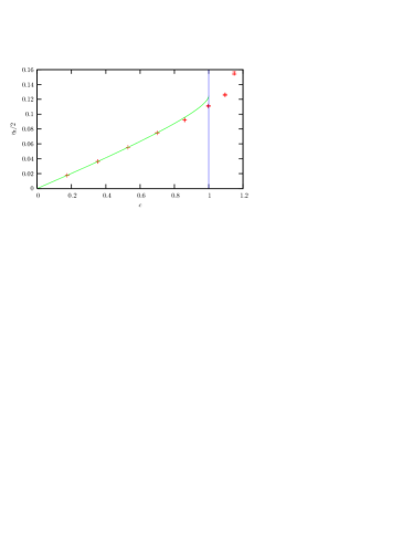
Figure 1: Our analytic prediction for the tricritical exponent $\eta_{\mathrm{t}}$ (solid line) as a function of the central charge $c$ compared with high-precision MC data (marks with error bars) bloeteetal . Our prediction extends only to $c=1$, indicated by the vertical line, while the numerical results continue to the tricritical O(2) model with $c=1.149(1)$ bloeteetal .

The tricritical HT graphs, representing simultaneously the hulls of FK clusters, have a distribution again of the form (2), characterized by two exponents $\sigma_{\mathrm{G}}^{\mathrm{t}},\tau_{\mathrm{G}}^{\mathrm{t}}$. Given our result (13) for the fractal dimension of these graphs, $\tau_{\mathrm{G}}^{\mathrm{t}}$ is determined exactly through Eq. (3) with $\tau_{\mathrm{G}}$ and $D_{\mathrm{G}}$ replaced by their tricritical counterparts $\tau^{\mathrm{t}}_{\mathrm{G}}$ and $D^{\mathrm{t}}_{\mathrm{G}}$.

In conclusion, we have shown that for $-2\leq N\leq 2$ the fractal structure of 2D HT graphs of the O($N$) spin model encodes the O($N$) critical behavior. We thereby extended de Gennes’ result for self-avoiding loops in the limit $N\to 0$ to random loops for arbitrary $-2\leq N\leq 2$. We studied the loops also close to the point where they collapse, corresponding to the HT representation of the tricritical O($N$) model. The fractal structure of the tricritical loops was argued to be in one-to-one correspondence with that of the critical loops, allowing us to also predict the magnetic scaling dimension $x^{\mathrm{t}}_{h}=\eta_{\mathrm{t}}/2=2h_{m/2,m/2}$ at the O($N)$ tricritical point, in very good agreement with recent MC data in the range $0\leq c\lesssim 0.7$.

The authors thank H. Blöte, C. von Ferber, Y. Holovatch, and B. Nienhuis for useful discussions and communications. This work is partially supported by the DFG grant No. JA 483/17-3 and by the German-Israel Foundation (GIF) under grant No. I-653-181.14/1999.

References

- (1)
- (2) H. E. Stanley, Introduction to Phase Transitions and Critical Phenomena (Oxford University Press, New York, 1971).
- (3) P. G. de Gennes, Phys. Lett. A 38, 339 (1972).
- (4) W. Janke and A. M. J. Schakel, Nucl. Phys. B 700 [FS], 385 (2004); Comp. Phys. Comm. 169, 222 (2005).
- (5) For an alternative numerical estimate of , using Eq. (2) at criticality, see V. S. Dotsenko et al., Nucl. Phys. B 448 [FS], 577 (1995).
- (6) W. Guo, H. W. J. Blöte, and Y.-Y. Liu, Commun. Theor. Phys. (Beijing) 41, 911 (2004).
- (7) E. Domany et al., Nucl. Phys. B 190, 279 (1981).
- (8) B. Nienhuis, Phys. Rev. Lett. 49, 1062 (1982); J. Stat. Phys. 34, 731 (1984).
- (9) D. Stauffer and A. Aharony, Introduction to Percolation Theory, 2nd edition (Taylor & Francis, London, 1994).
- (10) R. Balian and G. Toulouse, Phys. Rev. Lett. 30, 544 (1973).
- (11) B. Nienhuis, in: Phase Transitions and Critical Phenomena, edited by C. Domb and J. L. Lebowitz (Academic, London, 1987), Vol. 11, p. 1.
- (12) For consistency with Ref. geoPotts , we adopt here the notation (apart from normalization) of the stochastic Loewner evolution (SLEκ) formalism which puts various known results cited below on a mathematical rigorous footing. Specifically, . For an overview on SLEκ, see O. Schramm, Israel J. Math. 118, 221 (2000); S. Rohde and O. Schramm, Ann. Math. 161, 879 (2005); B. Duplantier, J. Stat. Phys. 110, 691 (2003).
- (13) C. Vanderzande, J. Phys. A 25, L75 (1992).
- (14) I. Jensen, J. Phys. A 36, 5731 (2003).
- (15) J. des Cloizeaux, Phys. Rev. A 10, 1665 (1974).
- (16) A. Coniglio et al., Phys. Rev. B 35, 3617 (1987).
- (17) B. Duplantier and H. Saleur, Phys. Rev. Lett. 58, 2325 (1987).
- (18) B. Duplantier and H. Saleur, Phys. Rev. Lett. 59, 539 (1987); ibid. 62, 1368 (1989).
- (19) R. B. Potts, Proc. Camb. Phil. Soc. 48, 106 (1952).
- (20) C. M. Fortuin and P. W. Kasteleyn, Physica 57, 536 (1972).
- (21) Y. Deng, H. W. J. Blöte, and B. Nienhuis, Phys. Rev. E 69, 026123 (2004).
- (22) B. Duplantier and H. Saleur, Phys. Rev. Lett. 63, 2536 (1989).
- (23) A. B. Zamolodchikov, Sov. J. Nucl. Phys. 44, 529 (1986).
- (24) W. Guo, H. W. J. Blöte, and B. Nienhuis, Int. J. Mod. Phys. C 10, 291 (1999).