Optical sum rules that relate to the potential energy of strongly correlated systems

Abstract

A class of sum rules for inelastic light scattering is developed. We show that the first moment of the non-resonant response provides information about the potential energy in strongly correlated systems. The polarization dependence of the sum rules provide information about the electronic excitations in different regions of the Brillouin zone. We determine the sum rule for the Falicov-Kimball model, which possesses a metal-insulator transition, and compare our results to the light scattering experiments in SmB₆.

One of the key signatures of strong electron correlations in condensed matter systems is the redistribution of spectral weight from low to high energies. A classic example of this phenomenon occurs when a normal metal becomes a superconductor at low temperatures. The optical conductivity is suppressed at low energy due to the presence of the superconducting gap richards_tinkham . Because there is an optical sum rule—the $f$-sum rule—which constrains the integrated spectral weight in $\sigma(\nu)$, the spectral weight suppressed below the superconducting energy gap reappears as a delta function peak at $\omega=0$, reflecting the onset of many-body coherence in the system. In high temperature superconductors, low-energy spectral weight has also been observed to shift to high energies below the superconducting transition htsc_oc . This dramatic spectral weight transfer is believed to be a signature of the strong electronic correlations in these and related materials Osafune .

The use of sum rules in optical conductivity measurements has had a wide impact in a number of fields of science. The optical sum rule originated in atomic physics as a relationship between the total number of electrons in the atomic system and the integrated spectral weight f-sum-rule . In a solid state system, the optical sum rule is usually projected onto the lowest energy band. In this case, the integrated spectral weight associated with electrons in the lowest band is related to the average kinetic energy of the electrons, regardless of the nature of the electronic interactions maldague . Since the electronic kinetic energy usually varies on an energy scale on the order of electron volts, the average kinetic energy is essentially a constant at low to moderate temperatures, and so the optical conductivity sum rule is essentially temperature-independent.

It would be useful to have similar sum rules that relate to the potential energy. In strongly correlated electron systems in which electronic interaction energies are on the order of, or greater than, the kinetic energy, efforts to study the potential energy as functions of doping, pressure, or temperature have been hindered by the limited tools available for measuring dynamical properties. We show here that the non-resonant inelastic light scattering response has sum rules similar to the f-sum rule that relate to the potential energy, and that these sum rules should provide valuable insight into the scattering of optical or x-ray photons from materials RIXS . As an added benefit compared to optical conductivity measurements, inelastic light scattering allows one to probe the electronic excitations in different regions of the Brillouin zone (BZ) by orienting the incident and scattered light polarizations.

Shastry and Shraiman shastry_shraiman were the first to point out that, if the self energy is local and $d\rightarrow\infty$, the optical conductivity and the nonresonant Raman response function in the depolarized ($\epsilon_{I}$ perpendicular to $\epsilon_{S}$) scattering geometry are related according to $\sigma(\nu)\propto S(\nu)/\nu$ a relationship that was proved in Ref. freericks_devereaux . This result implies that there is also a sum rule for Raman scattering, which is related to the f-sum rule for optical conductivity and to the average kinetic energy of the electrons.

In this paper, we show that there are also interaction-dependent sum rules for inelastic light scattering that are related to the potential energy for ${\bf q}=0$ Raman scattering, and to combinations of the potential and kinetic energies for ${\bf q}\neq 0$ inelastic x-ray scattering.

The formalism used to derive these sum rules is straightforward. If we consider the time-ordered product that yields the susceptibility corresponding to the fluctuations of an operator ${\mathcal{O}}$

$$\chi(\tau)={\rm Tr}\langle{\mathcal{T}}_{\tau}e^{-\beta{\mathcal{H}}}{\mathcal{O}}(\tau){\mathcal{O}}^{\dagger}(0)\rangle/{\mathcal{Z}}-\left({\rm Tr}\langle e^{-\beta{\mathcal{H}}}{\mathcal{O}}\rangle/\mathcal{Z}\right)^{2},$$ (1)

where $\tau$ is the imaginary time, ${\mathcal{H}}$ is the Hamiltonian, $\beta$ is the inverse temperature, ${\mathcal{Z}}={\rm Tr}e^{-\beta{\mathcal{H}}}$ is the partition function and ${\mathcal{O}}(\tau)=e^{\tau{\mathcal{H}}}{\mathcal{O}}e^{-\tau{\mathcal{H}}}$. Then it is easy to show from the spectral formula that when the susceptibility is Fourier transformed, and analytically continued to the real frequency axis, we get

$$\int_{0}^{\infty}d\nu\nu{\rm Im}\chi(q,\nu)=\frac{\pi}{2}{\rm Tr}\langle e^{-\beta{\mathcal{H}}}[{\mathcal{O}},[{\mathcal{H}},{\mathcal{O}}^{\dagger}]]\rangle/{\mathcal{Z}}$$ (2)

as the general sum rule for the first moment of the susceptibility (the brackets indicate commutators). If we consider the polarization operator ${\mathcal{O}}_{\rm pol}=e\sum_{i}{\bf R_{i}}n_{i}$ with $n_{i}$ the number density operator at site $i$, then this gives the $f$-sum rule where $\sigma(\nu)={\rm Im}\chi_{JJ}(\nu)/\hbar\nu$ in terms of the current-current correlation function $\chi_{JJ}$ (with $J=i[{\mathcal{H}},{\mathcal{O}}_{\rm pol}]/\hbar$:

$$\int_{0}^{\infty}d\nu\sigma(\nu)=\frac{\pi e^{2}a^{2}}{2\hbar}{\rm Tr}\langle e^{-\beta{\mathcal{H}}}(-\hat{T})\rangle/{\mathcal{Z}}.$$ (3)

The sum rule is proportional to the average kinetic energy (we consider only nearest neighbor hopping on a hypercubic lattice $\hat{T}=-t\sum_{i,\delta,\sigma}c_{i,\sigma}^{\dagger}c_{i+\delta,\sigma}$ with $\delta$ a nearest-neighbor translation vector). Likewise, if we consider the dynamical charge susceptibility ${\mathcal{O}}_{\rm ch}({\bf q})=\sum_{k}c^{\dagger}_{{\bf k}+{\bf k}/2,\sigma}c_{{\bf k}-{\bf q}/2,\sigma}$ we obtain

$$\int_{0}^{\infty}d\nu\nu{\rm Im}\chi_{ch}({\bf q},\nu)=$$

$$\frac{\pi}{2}Tr\langle e^{-\beta H}\sum_{\bf k}[\epsilon({\bf k+q})+\epsilon({\bf k-q})-2\epsilon({\bf k})]\rangle/{\mathcal{Z}},$$

$$=\pi(1-X){\rm Tr}\langle e^{-\beta{\mathcal{H}}}(-\hat{T})\rangle/{\mathcal{Z}},\quad{\rm(in~{}}d\rightarrow\infty{\rm)}$$ (4)

with $X=\lim_{d\rightarrow\infty}\sum_{i=1}^{d}\cos(k_{i})/d$ and $\epsilon({\bf q})$ the band structure. This vanishes as $q^{2}$ for ${\bf q}$=0 as it must, due to total charge conservation.

There is, however, no charge conservation for inelastic light scattering with ${\bf q}=0$ optical photons (Raman scattering). Raman scattering can be classified into representations of the irreducible point group symmetry of the crystal, selected by orienting the incident and scattered polarization vectors. The light scattering polarizations allow energy fluctuations to be projected onto different regions of the BZ, which has been useful in elucidating the behavior of electron dynamics for different momentum states old_papers . For example, for nonresonant scattering in tetragonal systems, the operator $\mathcal{O}_{A_{\rm 1g}}({\bf q})=\sum_{\bf k}\epsilon({\bf k})c^{\dagger}_{{\bf k}+{\bf q}/2}c_{{\bf k}-{\bf q}/2}=\hat{T}({\bf q})$ is the kinetic energy operator for ${\bf q}=0$ $A_{\rm 1g}$ scattering, and ${\mathcal{O}}_{B_{\rm 1g}}({\bf q})=\sum_{\bf k}\epsilon({\bf k}+{\bf Q})c^{\dagger}_{{\bf k}+{\bf q}/2}c_{{\bf k}-{\bf q}/2}$ is a modified kinetic energy operator for ${\bf q}=0$ $B_{\rm 1g}$ scattering for the zone boundary wavevector ${\bf Q}=(\pi,0)$ [which is generalized to higher dimensions as ${\bf Q}=(\pi,0,\pi,0,...)$]. Thus the $A_{1g}$ scattering response is associated with energy fluctuations from all regions of the BZ, while the $B_{\rm 1g}$ response is associated with dynamics near the BZ edges and away from the diagonals. The sum rule in Eq. (2) for nonresonant light scattering is similar to the optical sum rule, except the (model-dependent) operator average is different, and now depends on the potential energy since ${\mathcal{H}}=T+V$ [see Eq. (2)]. In the general case, there are two contributions—one from the kinetic energy commutator and one from the potential energy commutator:

$$\int_{0}^{\infty}d\nu\nu{\rm Im}\chi_{in}({\bf q},\nu)=\frac{\pi}{2{\mathcal{Z}}}{\rm Tr}\langle e^{-\beta{\mathcal{H}}}[\hat{T}({\bf q,Q})+\hat{U}({\bf q,Q})]\rangle.$$ (5)

The first term on the right-hand side of Eq. (5) does not depend on the type of Hamiltonian and is given by $\hat{T}({\bf q,Q})=-\sum_{{\bf k},\sigma}t({\bf k,q,Q})c^{\dagger}_{{\bf k},\sigma}c_{{\bf k},\sigma}$, with $t({\bf k,q,Q})=\epsilon({\bf k-Q-q/2})^{2}[\epsilon({\bf k-q})-\epsilon({\bf k})]+\epsilon({\bf k-Q+q/2})^{2}[\epsilon({\bf k+q})-\epsilon({\bf k})]$. Regardless of the symmetry [${\bf Q}=0$ for $A_{1g}$ or $(\pi,0)$ for $B_{1g}$] the kinetic-energy part of the sum rule does not contribute to the $({\bf q}=0)$ Raman scattering response, but it does contribute to the $({\bf q}\neq 0)$ inelastic X-ray scattering response in a polarization-dependent manner.

However the second term in Eq. (5) depends on the particular choice for the potential energy in the Hamiltonian. Evaluating these sum rules for different models is complicated, because the operator averages involve complex correlation functions. We consider the simplest model here, the spinless Falicov-Kimball model (FK) falicov_kimball

$$H_{FK}=-\frac{t^{*}}{2\sqrt{d}}\sum_{\langle i,j\rangle}c^{\dagger}_{i}c_{j}+U\sum_{i}c^{\dagger}_{i}c_{i}w_{i}.$$ (6)

Here $c^{\dagger}_{i}$ ($c_{i}$) creates (destroys) a conduction electron at site $i$, $w_{i}$ is a classical variable (representing the localized electron number at site $i$) that equals 0 or 1, $t^{*}$ is a renormalized hopping matrix that is nonzero between nearest neighbors on a hypercubic lattice in $d$-dimensions metzner_vollhardt , $U$ is the local screened Coulomb interaction between conduction and localized electrons, and $\langle i,j\rangle$ denotes a sum over sites $i$ and nearest neighbors $j$. In our calculations, the average filling for conduction and localized electrons is set to $1/2$. The FK model can be thought of as a limit of the Hubbard model for which one species of spin is not allowed to hop.

For the FK model, the operator $\hat{U}$ in the sum rule is

$$\hat{U}_{FK}({\bf q,Q})=\frac{Ut^{*2}}{2dN}\sum_{{\bf i,\delta,\delta^{\prime}}}c^{\dagger}_{i}c_{i+\delta+\delta^{\prime}}e^{-i{\bf Q}\cdot({\bf\delta+\delta^{\prime}})}$$ (7)

$$\times[e^{-i{\bf\frac{q}{2}}\cdot({\bf\delta+\delta^{\prime}})}(w_{{\bf i+\delta^{\prime}}}-w_{{\bf i+\delta+\delta^{\prime}}})-e^{i{\bf\frac{q}{2}}\cdot({\bf\delta+\delta^{\prime}})}(w_{\bf i}-w_{{\bf i+\delta}})].$$

This operator involves the difference of correlated hopping operators, where the hopping of the conduction electrons is correlated with the presence of the localized electrons; note how the potential energy directly enters when $\delta+\delta^{\prime}=0$. The operator for the Hubbard model is similar, but involves complex spin and spin-flip hopping correlation functions, which could be measured, in principle, with neutron scattering. It is surprising that the sum rule for a charge response function can be related to a spin response function in the Hubbard model.

The result in Eq. (Optical sum rules that relate to the potential energy of strongly correlated systems) is valid for any dimension. It can be evaluated exactly by examining the large dimensional limit using results from dynamical mean field theory (DMFT) fk_rev . The result for the FK model is

$$\int_{0}^{\infty}d\nu\nu {\rm Im} \chi_{in}({\bf q},\nu)=\frac{\pi}{2{\mathcal{Z}}}{\rm Tr}\langle\hat{T}({\bf q,Q})+\hat{U}({\bf q,Q})\rangle=$$ (8)

$${\rm Im}\int d\omega f(\omega)\left\{(1-X)X^{\prime 2}\left[1-\frac{3}{2}Z(\omega)G(\omega)-Z^{2}(\omega)\left[1-Z(\omega)G(\omega)\right]\right]+\frac{1}{2}(X-1)[1-Z(\omega)G(\omega)]\right\}$$

$$+{\rm Im}\int d\omega f(\omega)(\Sigma(\omega)-U\langle w_{i}\rangle)\left\{\frac{1-X^{\prime 2}}{2}G(\omega)+\left\{Z(\omega)-1/G(\omega)\right\}X^{\prime 2}\right\},$$

with $f(\omega)=1/[1+\exp(\beta\omega)]$ the Fermi function, $G(\omega)$ and $\Sigma(\omega)$ the Green’s function and self energy, respectively, and $Z(\omega)=\omega+\mu-\Sigma(\omega)$. The difference between $A_{\rm 1g}$ and $B_{\rm 1g}$ scattering comes from the momentum factors $X^{\prime}=\lim_{d\rightarrow\infty}(1/d)\sum_{i=1}^{d}\cos(q_{i}/2)h^{i}$, with $h=1$ ($-1)$ for $A_{\rm 1g}$ ($B_{\rm 1g}$) scattering. Note that both the first term associated with the kinetic energy and the second term associated with the potential energy contribute to the sum rule for inelastic x-ray scattering (${\bf q}\neq 0$). On the other hand, only the second “potential energy” term contributes to the sum rule for Raman scattering (${\bf q}=0$). Therefore, the sum rule’s momentum dependence contains information regarding the potential and kinetic energy contributions.

Note that the sum rule for $(X=1)$ Raman scattering is proportional to the correlated part of the self energy, due to the factor $\Sigma(\omega)-U\langle w_{i}\rangle$ which has the Hartree shift subtracted off. The term in wavy brackets can be viewed as a Green’s-function weighted variance of the bandstructure for $A_{\rm 1g}$ scattering, which can be interpreted as a measure of the width of the strongly-correlated band. Further, we note that in DMFT, where the self energy is local (and $d\rightarrow\infty)$, the sum rule for $B_{\rm 1g}$ Raman scattering would also apply to the second moment of the optical conductivity:

$$\int_{0}^{\infty}d\nu\nu{\rm Im}\chi_{B_{1g}}({\bf q}=0,\nu)\propto\int_{0}^{\infty}d\nu\nu^{2}\sigma(\nu).$$ (9)

However, this relationship is violated if there is any momentum dependence associated with the self-energy or in finite dimensions.

We plot the sum rule for the FK model in Fig. 1 for $B_{\rm 1g}$ Raman scattering (${\bf q}=0$) and different values of $U$ as a function of temperature (results for $A_{\rm 1g}$ are similar). We have checked that an explicit integral of the nonresonant Raman response agrees with the sum rule plotted in Fig. 1 for many different values of $U$ and $T$. We expect similar results to hold for other models of correlated electrons like the Hubbard model. Fig. 1 shows that these sum rules are essentially constant at low temperature, indicating (i) the sum rule can be used to calibrate data from different samples and different temperatures; (ii) the sum rule can be used to determine the frequency above which interband transitions become prominent; (iii) the Raman response function multiplied by the frequency should be used to track spectral weight shifts because of the sum rule; and (iv) the sum rules have a momentum dependence for inelastic x-ray scattering that can be calculated and compared to experiment. Note that unlike the f-sum rule, which is evenly weighted throughout the spectral range, the Raman sum rules are heavily weighted at higher energies due to the multiplication by the frequency. Consequently, unless there is a clear separation between low and high energy bands in the system, higher energy bands can significantly distort the sum rule.

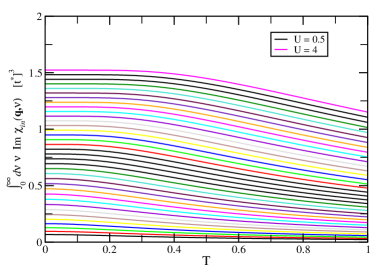
Figure 1: $B_{\rm 1g}$ sum rules as a function of temperature for the spinless FK model solved within DMFT (the $A_{\rm 1g}$ results are similar). The different curves correspond to different values of the interaction strength increasing in steps of 0.1 from 0.5 on the lowest curve to 4.0 on the highest curve.

The momentum dependence of the sum rule is reduced as $U$ increases and the physical properties become more local. The sum rule generally increases for increasing momentum transfer since the kinetic energy term in Eq. (8) contributes to the sum rule as phase space is created for light scattering by increasing ${\bf q}$.

The underlying MIT is revealed via a simple scaling analysis, shown in Fig. 2. It can be shown that for metallic systems the sum rule varies as $U^{2}$ for small $U$, with large deviations occuring as the MIT is approached. In Fig. 2 we plot the sum rule divided by $U^{2}$ for different temperatures as a function of $U$. We see that the sum rule data collapses for small $U$ onto a single line for all temperatures. The scaled data abruptly fans out from the straight line at approximately $U=U_{c}$ and a strong temperature dependence emerges for larger $U$. Thus the onset of a strong temperature dependence and deviations from $U^{2}$ scaling can be used as a straightforward and quantitative way to identify a MIT from the optical data.

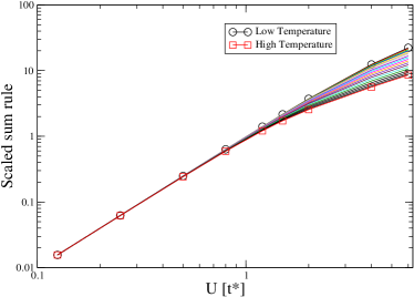
Figure 2: $B_{\rm 1g}$ scaled sum rules showing the scaling behavior with $U^{2}$ for the FK model discussed in the text. Deviations in scaling occur when $U\geq U_{c}=\sqrt{2}t^{*}$, the critical value of $U$ for the metal-insulator transition in the half-filled FK model.

We show the relevance of these sum rules to an experimental system that is ideal for this situation, SmB₆. The Raman results on SmB₆ provide an ideal comparison to this model for several reasons: the spectra have a clear separation between the low energy (intraband) and high energy (interband) scattering contributions; only the low energy component in SmB₆ exhibits significant spectral weight changes due to the gap formation at low temperatures; and the photon energy used in the experiment lies in a gap in the density of states of SmB₆, and therefore the Raman response is not likely to be influenced by resonant or mixed-scattering effects. When we take the Raman data, and multiply by the frequency, we find that the sum rule holds to within five percent in this system (see Fig. 3), confirming the behavior determined from the FK model in DMFT (Fig. 1).

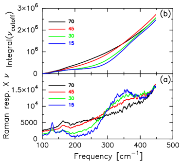
Figure 3: Raman response multiplied by frequency for SmB₆ at four different temperatures. On top is a plot of the integrated sum rule as a function of the frequency cutoff. Both curves are plotted in arbitrary units. The near crossing of the curves in the upper panel indicates where a cutoff can be placed (since the higher energy bands have little $T$ dependence, the curves become parallel at high frequency, because the response is the same for all $T$).

In summary, we have discovered a class of sum rules for inelastic light scattering that are useful in analysing both Raman scattering and inelastic x-ray scattering. The sum rules depend crucially on the form of the electron interactions, and thereby yield useful information about the correlations in the material. While light scattering data on correlated metals or insulators is still rather limited (particularly with regard to inelastic X-ray scattering), our class of sum rules may be employed to analyze data and elucidate how the kinetic and potential energy of the system evolves as a function of doping, pressure, or temperature.

References

- (1) P. L. Richards and M. Tinkham, Phys. Rev. Lett. 1, 318 (1958).
- (2) J. E. Hirsch, Physica C201, 347 (1992); D. N. Basov, et al., Science 283, 49 (1999); J. E. Hirsch and F. Marsiglio, Phys. Rev. B 62, 15131 (2000); J. E. Hirsch, Science 295, 2226 (2002); H. J. A. Molegraaf, et al., Science 295, 2239 (2002); A. B. Kuzmenko, et al., Phys. Rev. Lett. 91, 037004 (2003).
- (3) T. Osafune, et al., Phys. Rev. Lett. 82, 1313 (1999).
- (4) W. Thomas, Naturwiss. 13, 627 (1925); W. Kuhn, Z. Phys. 33, 408 (1925).
- (5) P. F. Maldague, Phys. Rev. B 16, 2437 (1977).
- (6) We note that a symmetry dependent sum-rule for resonant inelastic x-ray scattering in a single-ion model has been considered in M. van Veenendaal, P. Carra, and B. T. Thole, Phys. Rev. B 54, 16 010 (1996) and F. Borgatti et al., Phys. Rev. B 69, 134420 (2004). However these treatments can not be applied to systems near a metal-insulator transition nor to systems in which nonresonant scattering is important.
- (7) B. S. Shastry and B. I. Shraiman, Phys. Rev. Lett. 65, 1068 (1990); Int. J. Mod. Phys. B 5, 365 (1991).
- (8) J. K. Freericks and T. P. Devereaux, Phys. Rev. B 64, 125110 (2001).
- (9) F. Venturini et al., Phys. Rev. Lett. 89, 107003 (2002).
- (10) L. M. Falicov and J. C. Kimball, Phys. Rev. Lett. 22, 997 (1969).
- (11) W. Metzner and D. Vollhardt, Phys. Rev. Lett. 62, 324 (1989).
- (12) J. K. Freericks and V. Zlatić, Rev. Mod. Phys. 75, 1333 (2003).
- (13) P. Nyhus, S.L. Cooper, Z. Fisk, and J. Sarrao, Phys. Rev. B 52, R14308 (1995); 55, 12488 (1997).