Optimal spin-entangled electron-hole pair pump

Abstract

A nonperturbative theory is presented for the creation by an oscillating potential of spin-entangled electron-hole pairs in the Fermi sea. In the weak potential limit, considered earlier by Samuelsson and Büttiker, the entanglement production is much less than one bit per cycle. We demonstrate that a strong potential oscillation can produce an average of one Bell pair per two cycles, making it an efficient source of entangled flying qubits.

The quantum electron pump is a device that transfers electrons phase coherently between two reservoirs at the same voltage, by means of a slowly oscillating voltage on a gate electrode Swi99 . Special pump cycles exist that transfer the charge in a quantized fashion, one $e$ per cycle Shu00 ; Lev01 ; Avr01 ; Mak01 . Building on earlier proposals to stochastically produce entangled electron-hole pairs in a Fermi sea out of equilibrium Bee03 ; Sam04a , Samuelsson and Büttiker have proposed Sam04 that a quantum pump could be used to create entangled Bell pairs in a controlled manner, clocked by the gate voltage. Such a device could be a building block of quantum computing designs using ballistic flying qubits in nanowires or in quantum Hall edge channels Ber00 ; Ion01 ; Bar04 .

To find out how close one get to this ideal, one needs to go beyond the perturbation theory of Ref. Sam04 — in which the number of Bell pairs per cycle is $\ll 1$. A nonperturbative theory of the quantum entanglement pump is presented here. We show that the entanglement production is closely related to the charge noise, to the extent that a noiseless pump produces no entanglement. By maximizing the charge noise with spin-independent scattering we calculate that a pump can produce, on average, 1 Bell pair every 2 cycles. A deterministic spin-entangler Bee04 , being the analogue of a quantized charge pump, would have an entanglement production of $1$ Bell pair per cycle, so the optimal entanglement pump has one half the efficiency of a deterministic entangler.

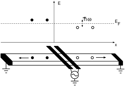
We consider a two-channel phase coherent conductor, see Fig. 1, connecting a left and a right electron reservoir in thermal equilibrium (same temperature $T$ and Fermi energy $E_{F}$ in each reservoir). The two channels may refer to an orbital or to a spin degree of freedom. (To be definite, we will usually speak of a spin degree of freedom.) A periodically varying time-dependent electrical potential $V(\mathbf{r},t)$ (with period $2\pi/\omega$) excites electron-hole pairs in the Fermi sea of the conductor. The quantum mechanical state of an electron-hole pair, at energies $E,E^{\prime}$ differing by a multiple of $\hbar\omega$, may be entangled in the channel indices. The entanglement can be a resource for quantum computing if the electron and the hole excitation are scattered to opposite ends of the conductor, so that they become two separate qubits. We wish to relate this entanglement production to the scattering matrix of the conductor.

Figure 1: Production of entangled electron-hole pairs in a narrow ballistic conductor by a quantum electron pump. The left and right ends of the conductor are at the same potential, while the potential on the gate electrodes at the center is periodically modulated. Such a device produces spatially separated electron-hole pairs (black and white circles), differing in energy by a multiple of the pump frequency $\omega$. For spin-independent scattering the electron ($e$) and hole ($h$) produced during a given cycle have the same spin $\uparrow,\downarrow$, so that their wave function is that of a Bell pair, $\propto|\!\uparrow_{e}\uparrow_{h}\rangle+|\!\downarrow_{e}\downarrow_{h}\rangle$. The optimal quantum entanglement pump produces, on average, $1$ Bell pair every $2$ cycles.

The four characteristic energy scales of this problem are the thermal energy $k_{B}T$, the pump energy $\hbar\omega$, the Thouless energy $\hbar/\tau_{D}$ (set by the inverse of the mean dwell time $\tau_{D}$ of an electron in the conductor), and finally the Fermi energy $E_{F}$. In nanostructures at low temperatures, the characteristic relative magnitude of these energy scales is $k_{B}T\ll\hbar\omega\ll\hbar/\tau_{D}\ll E_{F}$. This is the adiabatic, low temperature regime in which we will work.

We seek a relation between the entanglement production and the scattering matrix $S$ of the pump, which is the unitary operator relating incoming to outgoing states:

$$b_{n}(E)=\sum_{m}\int\frac{dE^{\prime}}{2\pi}S_{nm}(E,E^{\prime})a_{m}(E^{\prime}).$$ (1)

Here $a_{n}(E)$ is the fermion annihilation operator for an incoming channel $n$ at energy $E$, and $b_{n}(E)$ is the annihilation operator for an outgoing channel. There are four channels in total ($n=1,2,3,4$), two in the left lead and two in the right lead. The Wigner transform of the scattering matrix Vav01 , defined by

$$S_{W}(E,t)=\int\frac{dE^{\prime}}{2\pi}\,S(E+E^{\prime}/2,E-E^{\prime}/2)e^{-iE^{\prime}t/\hbar},$$ (2)

depends on $E$ on the scale $\hbar/\tau_{D}$. In the adiabatic regime $\omega\tau_{D}\ll 1$ one may therefore neglect the $E$-dependence on the scale of the pump energy, approximating $S_{W}(E,t)\approx S_{W}(E_{F},t)\equiv{\cal S}(t)$. The $4\times 4$ unitary matrix ${\cal S}(t)$ can be obtained by solving the static scattering problem for the frozen potential $V({\bf r},t)$.

Within a single period $2\pi/\omega$ the excitation energies can only be resolved on the scale of $\hbar\omega$, so we discretize $E_{p}=p\hbar\omega$ with integer $p$. A pair of energies $E_{p}$ and $E_{q}$ is coupled by the Floquet matrix ${\cal F}(p-q)$, which is the Fourier transform of the Wigner transformed scattering matrix Mos02 ,

$${\cal F}(p-q)=\frac{\omega}{2\pi}\int_{0}^{2\pi/\omega}dt\,{\cal S}(t)e^{i(p-q)\omega t}.$$ (3)

The unitarity relation for the Floquet matrix reads

$$\sum_{n^{\prime},p^{\prime}}{\cal F}_{nn^{\prime}}^{\vphantom{\ast}}(p-p^{\prime}){\cal F}_{mn^{\prime}}^{\ast}(q-p^{\prime})=\delta_{nm}\delta_{pq}.$$ (4)

We assume zero temperature, so the incoming state $|\Psi_{0}\rangle$ is the unperturbed Fermi sea, consisting of all levels (left and right) doubly occupied below $E_{F}$ and empty above $E_{F}$:

$$|\Psi_{0}\rangle=\prod_{p}f(E_{p})\prod_{n}a^{\dagger}_{n}(E_{p})|0\rangle.$$ (5)

The state $|0\rangle$ is the vacuum and $f(E)=\theta(E_{F}-E)$ is the zero-temperature Fermi function. The outgoing state $|\Psi\rangle$ is obtained from $|\Psi_{0}\rangle$ by substituting Eq. (1) and taking the adiabatic approximation for the scattering matrix,

$$|\Psi\rangle=\prod_{p}f(E_{p})\prod_{n}\biggl{(}\sum_{p^{\prime}}\sum_{n^{\prime}}b^{\dagger}_{n^{\prime}}(E_{p^{\prime}}){\cal F}_{n^{\prime}n}(p^{\prime}-p)\biggr{)}|0\rangle.$$ (6)

We denote by $w_{pq}^{eh}$ the probability that the pump excites within one cycle a single electron-hole pair, consisting of an electron at the left at an energy $E_{p}$ above the Fermi level and a hole at the right at an energy $E_{q}$ below the Fermi level. The entanglement entropy (or entanglement of formation) of the spins is denoted by ${\cal E}_{pq}^{eh}$ (measured in bits per cycle). Similarly, $w_{qp}^{he}$ and ${\cal E}_{qp}^{he}$ refer to a hole at the left and an electron at the right. The average production, per cycle, of spin-entangled electron-hole pairs is

$${\cal E}=\sum_{E_{p}>E_{F}}\sum_{E_{q}<E_{F}}\bigl{(}w_{pq}^{eh}{\cal E}_{pq}^{eh}+w_{qp}^{he}{\cal E}_{qp}^{he}\bigr{)}.$$ (7)

A maximally entangled Bell pair has ${\cal E}_{pq}^{eh}=1$, so it contributes $w_{pq}^{eh}$ bits to the entanglement production.

The weight factor $w_{pq}^{eh}$ and entanglement entropy ${\cal E}_{pq}^{eh}$ of an electron-hole pair can both be calculated by projecting $|\Psi\rangle$ onto a state ${\cal P}_{pq}^{eh}|\Psi\rangle$ with all levels (left and right) empty above $E_{F}$ and doubly occupied below $E_{F}$ — except for a singly occupied level $E_{p}>E_{F}$ at the left and $E_{q}<E_{F}$ at the right. The (unnormalized) projected electron-hole state has the form

$${\cal P}_{pq}^{eh}|\Psi\rangle=\sum_{\sigma,\sigma^{\prime}=\uparrow,\downarrow}\alpha_{\sigma\sigma^{\prime}}b^{\dagger}_{L\sigma}(E_{p})b^{\dagger}_{R\sigma^{\prime}}(E_{q})|0\rangle.$$ (8)

The four channels have been labeled $L\!\!\uparrow,L\!\!\downarrow,R\!\!\uparrow,R\!\!\downarrow$, where $L,R$ refers to the left and right lead and the arrows $\uparrow,\downarrow$ indicate the spin. The $2\times 2$ matrix $\alpha$ determines the weight factor as well as the entanglement entropy,

$${\cal E}_{pq}^{eh}=-x\log_{2}x-(1-x)\log_{2}(1-x),$$

$$\qquad x={\tfrac{1}{2}}+{\tfrac{1}{2}}\sqrt{1-{\cal C}^{2}},$$ (9)

$$w_{pq}^{eh}={\rm Tr}\,\alpha\alpha^{\dagger},\;\;{\cal C}=\frac{2({\rm Det}\,\alpha\alpha^{\dagger})^{1/2}}{{\rm Tr}\,\alpha\alpha^{\dagger}}.$$ (10)

The number ${\cal C}\in[0,1]$ is the concurrence Woo98 of the electron-hole pair.

In order to calculate the matrix $\alpha$ it is more convenient to perform the algebraic manipulations on the pair correlator $K$ in the outgoing state $|\Psi\rangle$, rather than on the state itself. The pair correlator fully characterizes the outgoing state (6) because it is Gaussian, meaning that higher order correlators in normal order (all $b^{\dagger}$’s to the left of the $b$’s) are constructed from the pair correlator according to the rule of Gaussian averages. The correlator is given in terms of the Floquet matrix by

$$K_{nm}(p,q)=\langle b_{m}^{\dagger}(E_{q})b_{n}^{\vphantom{\dagger}}(E_{p})\rangle$$

$$\qquad=\sum_{n^{\prime},p^{\prime}}{\mathcal{F}}_{nn^{\prime}}^{\vphantom{\ast}}(p-p^{\prime})f(E_{p^{\prime}}){\mathcal{F}}_{mn^{\prime}}^{\ast}(q-p^{\prime}).$$ (11)

The matrix $K$ is Hermitian and idempotent in the joint set of energy and channel indices: $K=K^{\dagger}=K^{2}$. This signifies that the state it represents is a pure (rather than a mixed) state note2 .

Projection of $|\Psi\rangle$ onto a set of filled or empty levels preserves the Gaussian property. The correlator $\bar{K}$ of the projected state ${\cal P}_{pq}|\Psi\rangle$ is derived from $K$ by the procedure known in matrix algebra as Gaussian elimination Eis02 . By interchanging rows and columns of the matrix $K$ we move the indices $pL\!\!\uparrow,pL\!\!\downarrow,qR\!\!\uparrow,qR\!\!\downarrow$ to the upper left hand corner, to obtain the block form

$$K=\begin{pmatrix}K_{\rm dir}&X\\ X^{\dagger}&Y\end{pmatrix},\;K_{\rm dir}=\begin{pmatrix}K_{LL}(p,p)&K_{LR}(p,q)\\ K_{RL}(q,p)&K_{RR}(q,q)\end{pmatrix}.$$ (12)

The $4\times 4$ block $K_{\rm dir}$ contains the direct coupling of the spin degenerate levels $p$ at the left and $q$ at the right. The correlator $\bar{K}$ contains in addition the indirect coupling via the filled or empty states in the block $Y$,

$$\bar{K}=K_{\rm dir}+X(1-Y-\Lambda)^{-1}X^{\dagger},$$ (13a)

$$\bar{w}\equiv\langle\Psi|{\cal P}_{pq}|\Psi\rangle=|{\rm Det}\,(1-Y-\Lambda)|.$$ (13b)

The diagonal matrix $\Lambda$ has a $1$ on the diagonal if the state is filled (below $E_{F}$) and a $0$ if it is empty (above $E_{F}$). A derivation of Eq. (13) is given in App. A.

One readily verifies that $\bar{K}^{2}=\bar{K}$, so the projection preserves the purity of the state, as it should. Since ${\cal P}_{pq}|\Psi\rangle$ contains a total of two electrons in four states, the correlator $\bar{K}$ has two eigenvalues equal to 1 and two eigenvalues equal to 0. We write $\bar{K}=U{\rm diag}\,(0,0,1,1)U^{\dagger}$, with $U$ the unitary matrix of eigenvectors. The projected state corresponding to the correlator $\bar{K}$ has the form

$${\cal P}_{pq}|\Psi\rangle=\bar{w}^{1/2}({\bf b}^{\dagger}U)_{R\uparrow}({\bf b}^{\dagger}U)_{R\downarrow}|0\rangle,$$ (14)

$${\bf b}=\bigl{(}b_{L\uparrow}(E_{p}),b_{L\downarrow}(E_{p}),b_{R\uparrow}(E_{q}),b_{R\downarrow}(E_{q})\bigr{)}.$$ (15)

The matrix $U$ plays the role of an effective scattering matrix for the two electrons in the two states left and right, including in addition to the direct scattering (described by the original scattering matrix $S$) also the indirect transitions via the other states.

To obtain the required projection ${\cal P}_{pq}^{eh}|\Psi\rangle$ we still need to project ${\cal P}_{pq}|\Psi\rangle$ onto a state with a single electron left and a single hole right, excluding the double occupation. (We could not do the projection in a single step because the final state (8) is not Gaussian, so it can not be represented by a pair correlator.) By comparing Eqs. (8) and (14) we can relate the coefficient matrices $U$ and $\alpha$ before and after projection,

$$\alpha=i\bar{w}^{1/2}U_{LR}\sigma_{y}U_{RR}^{T},\;\;U=\begin{pmatrix}U_{LL}&U_{LR}\\ U_{RL}&U_{RR}\end{pmatrix}.$$ (16)

(The matrix $\sigma_{y}$ is a Pauli matrix.) Substitution into Eqs. (9) and (10) then gives the contribution from this electron-hole pair to the entanglement production.

A major simplification occurs in the case of spin-independent scattering. Then $U_{LR}$ and $U_{RR}$ are proportional to the $2\times 2$ unit matrix $\openone$, so $\alpha\propto\sigma_{y}$ and the electron-hole pair is maximally entangled (${\cal E}_{pq}^{eh}=1$). In view of Eq. (7) the average entanglement production per cycle,

$${\cal E}=\sum_{E_{p}>E_{F}}\sum_{E_{q}<E_{F}}\bigl{(}w_{pq}^{eh}+w_{qp}^{he}\bigr{)},$$ (17)

is the probability that the pump produces a single spatially separated electron-hole pair in a given cycle.

The probability (17) can be rewritten as ${\cal E}=P_{0}^{\uparrow}P_{1}^{\downarrow}+P_{0}^{\downarrow}P_{1}^{\uparrow}$, where $P_{\nu}^{\sigma}$ is the probability that $\nu$ spatially separated electron-hole pairs of spin $\sigma$ are produced in a given cycle. From $0\leq P_{1}^{\uparrow}=P_{1}^{\downarrow}\leq 1-P_{0}^{\uparrow}=1-P_{0}^{\downarrow}\leq 1$ we deduce that

$${\cal E}\leq 2P_{0}^{\sigma}(1-P_{0}^{\sigma})\leq\tfrac{1}{2}.$$ (18)

This maximal entanglement ${\cal E}_{\rm max}=\frac{1}{2}$ of one half bit per cycle is reached for $P_{0}^{\uparrow}=P_{0}^{\downarrow}=P_{1}^{\uparrow}=P_{1}^{\downarrow}=\frac{1}{2}$. Eq. (18) is derived for spin-independent scattering. It seems unlikely that spin-dependent scattering (which reduces the entanglement per electron-hole pair) could violate the bound ${\cal E}\leq\frac{1}{2}$, but we have not been able to exclude this possibility on mathematical grounds.

To demonstrate that the optimal value ${\cal E}_{\rm max}=\frac{1}{2}$ can be reached, we consider the pump cycle

$${\cal S}(\tau)=\begin{pmatrix}e^{i\omega\tau}r&t\\ t^{\prime}&e^{-i\omega\tau}r^{\prime}\end{pmatrix},$$ (19)

which has been used as a model for a quantized charge pump Shu00 ; And00 . (A more general class of pump cycles Iva97 with the same entanglement production is analyzed in App. B.) Choosing the Fermi level such that $E_{0}<E_{F}<E_{1}$, Eq. (11) evaluates to

$$K(p,q) = \begin{pmatrix}\openone&0\\ 0&\openone\end{pmatrix}\delta_{pq}f(E_{p})$$ (20)

$$\mbox{}+\begin{pmatrix}-rr^{\dagger}\delta_{p0}\delta_{q0}&tr^{\prime\dagger}\delta_{p0}\delta_{q1}\\ r^{\prime}t^{\dagger}\delta_{p1}\delta_{q0}&r^{\prime}r^{\prime\dagger}\delta_{p1}\delta_{q1}\end{pmatrix}.$$

The only pair of coupled levels is $E_{0}$ at the left and $E_{1}$ at the right, so the entanglement production consists of a single term ${\cal E}=w_{01}^{he}{\cal E}_{01}^{he}$. The matrix $X$ in the decomposition (12) vanishes, and $Y=\Lambda$, hence Eq. (13) simplifies to

$$\bar{K}=K_{\rm dir}=\begin{pmatrix}\openone-rr^{\dagger}&tr^{\prime\dagger}\\ r^{\prime}t^{\dagger}&r^{\prime}r^{\prime\dagger}\end{pmatrix},\;\;\bar{w}=1.$$ (21)

Eq. (16) gives $\alpha=it\sigma_{y}r^{\prime T}$, which finally leads to the entanglement production

$${\cal E}=H(x_{1},x_{2}),\;\;x_{1}=T_{1}(1-T_{2}),\;\;x_{2}=T_{2}(1-T_{1}),$$ (22)

in terms of the function

$$H(x,y)=(x+y)\log_{2}(x+y)-x\log_{2}x-y\log_{2}y$$ (23)

of the two transmission eigenvalues $T_{1},T_{2}$ (eigenvalues of $tt^{\dagger}$, equal to the eigenvalues of $t^{\prime}t^{\prime\dagger}$ because of unitarity of ${\cal S}$).

The optimal entanglement production ${\cal E}_{\rm max}=\frac{1}{2}$ is reached in Eq. (22) for $T_{1}=T_{2}=\frac{1}{2}$ (corresponding to spin-independent scattering, as expected). This is also the choice of parameters at which the charge noise $\propto T_{1}(1-T_{1})+T_{2}(1-T_{2})$ is maximized And00 . Although entanglement entropy and charge noise are different physical quantities, with a different dependence on the transmission eigenvalues, quite generally one can state that there can be no entanglement production without charge noise. Indeed, a deterministic spin-independent charge pump has $P_{0}^{\sigma}=0$ hence ${\cal E}=0$, in view of Eq. (18).

A one-to-one relationship between entanglement production and charge noise is possible in the weak pumping limit of Ref. Sam04 . To demonstrate this, we quantify the pumping strength by a dimensionless parameter $\epsilon\ll 1$, and calculate both quantities to leading order in $\epsilon$. The Floquet matrix to first order has the general form

$${\cal F}(p-q)=\left\{\begin{array}[]{ll}{\cal F}_{0}&{\rm if}\;\;p=q,\\ i\epsilon Q{\cal F}_{0}&{\rm if}\;p=q+1,\\ i\epsilon Q^{\dagger}{\cal F}_{0}&{\rm if}\;p=q-1.\end{array}\right.$$ (24)

Unitarity of ${\cal F}_{0}$ ensures unitarity of ${\cal F}$ up to terms of order $\epsilon^{2}$. The corresponding correlator (11) is

$$K(p,q) = f(E_{p})\delta_{pq}+i\epsilon[f(E_{q})-f(E_{p})]\delta_{p,q+1}Q$$ (25)

$$\mbox{}-i\epsilon[f(E_{p})-f(E_{q})]\delta_{q,p+1}Q^{\dagger}.$$

Following the same steps as before, we arrive at the entanglement production

$${\cal E}=\epsilon^{2}H\bigl{(}y_{1},y_{2}\bigr{)}+\epsilon^{2}H\bigl{(}y^{\prime}_{1},y^{\prime}_{2}\bigr{)},$$ (26)

in terms of the function $H$ defined in Eq. (23). The numbers $y_{n}$ and $y^{\prime}_{n}$ are the eigenvalues of the matrices $\tau\tau^{\dagger}$ and $\tau^{\prime}\tau^{\prime\dagger}$, respectively, constructed from sub-blocks of the matrix

$$Q=\begin{pmatrix}\rho&\tau\\ \tau^{\prime}&\rho\end{pmatrix}.$$ (27)

In the case of spin-independent scattering $y_{1}=y_{2}\equiv y$, $y^{\prime}_{1}=y^{\prime}_{2}\equiv y^{\prime}$, and Eq. (26) simplifies to

$${\cal E}=2\epsilon^{2}(y+y^{\prime}).$$ (28)

To compare this result with the charge noise ${\cal P}$, we use the formula Mos02 ; And00 ; Pol02 ; note1

$${\cal P}=\frac{1}{4}\sum_{p=1}^{\infty}p\,{\rm Tr}\,G(p)G(-p),$$ (29)

$$G(p)=\sum_{q=-\infty}^{\infty}{\cal F}^{\dagger}(q-p)\begin{pmatrix}\openone&0\\ 0&-\openone\end{pmatrix}{\cal F}(q).$$ (30)

In the weak pumping limit this reduces to

$${\cal P}=\epsilon^{2}\bigl{(}y_{1}+y_{2}+y^{\prime}_{1}+y^{\prime}_{2}\bigr{)},$$ (31)

which equals the entanglement production (28) in the spin-independent case.

The close relation between entanglement production and charge noise in the weak pumping regime is consistent with the finding of Ref. Sam04 that low-frequency noise measurements can be used to detect the entanglement in this regime. To access the nonperturbative regime investigated in this paper requires time-resolved detection, on the time scale of $1/\omega$. The requirement that the thermal energy $k_{B}T$ remains less than $\hbar\omega$ poses a practical lower limit to the frequency. What motivates further efforts on the side of the detection is the relative simplicity on the side of the production: The quantum entanglement pump requires no advanced lithography or control over electron-electron interactions to produce as much as one Bell pair per two cycles.

This work was supported by the Dutch Science Foundation NWO/FOM and by the U.S. Army Research Office (Grant No. DAAD 19–02–0086).

Appendix A Gaussian elimination of fermion degrees of freedom

The Gaussian elimination of boson degrees of freedom was done in Ref. Eis02 . Here we perform the analogous calculation for fermions, leading to Eq. (13). We represent the density matrix $\rho$ by the normally ordered characteristic function

$$\chi(\bm{\xi})={\rm Tr}\,\rho\,e^{\bm{\xi}\cdot\bm{b}^{\dagger}}e^{\bm{\xi}^{\ast}\cdot\bm{b}}.$$ (32)

The entire set of fermion annihilation operators is contained in the vector $\bm{b}$. The characteristic function depends on the vector of Grassmann variables $\bm{\xi}$. For a Gaussian state, with pair correlator $\bm{K}$, one has

$$\chi(\bm{\xi})=\exp(\bm{\xi}^{\ast}\cdot{\bm{K}}\cdot\bm{\xi}).$$ (33)

We first eliminate a single degree freedom, labeled by a subscript $0$, by projecting onto a filled state. The projection operator is $b_{0}^{\dagger}b_{0}^{\vphantom{\dagger}}$, so the characteristic function after projection is

$$\chi_{0,{\rm filled}}(\bm{\xi}) = {\rm Tr}\,b_{0}^{\dagger}b_{0}^{\vphantom{\dagger}}\rho\,e^{\bm{\xi}\cdot\bm{b}^{\dagger}}e^{\bm{\xi}^{\ast}\cdot\bm{b}}$$ (34)

$$= \lim_{\xi_{0},\xi_{0}^{\ast}\rightarrow 0}\frac{d}{d\xi_{0}}\frac{d}{d\xi_{0}^{\ast}}\chi(\bm{\xi})$$

$$= \int d\xi_{0}\int d\xi_{0}^{\ast}\,\chi(\bm{\xi}).$$

The final equality holds because differentiation and integration is the same for Grassmann variables. Similarly, we can project onto an empty state, with projection operator $1-b_{0}^{\dagger}b_{0}^{\vphantom{\dagger}}$ and characteristic function

$$\chi_{0,{\rm empty}}(\bm{\xi}) = {\rm Tr}\,(1-b_{0}^{\dagger}b_{0}^{\vphantom{\dagger}})\rho\,e^{\bm{\xi}\cdot\bm{b}^{\dagger}}e^{\bm{\xi}^{\ast}\cdot\bm{b}}$$ (35)

$$= -\lim_{\xi_{0},\xi_{0}^{\ast}\rightarrow 0}\frac{d}{d\xi_{0}}\frac{d}{d\xi_{0}^{\ast}}e^{-\xi_{0}^{\ast}\xi_{0}^{\vphantom{\ast}}}\chi(\bm{\xi})$$

$$= -\int d\xi_{0}\int d\xi_{0}^{\ast}\,e^{-\xi_{0}^{\ast}\xi_{0}^{\vphantom{\ast}}}\chi(\bm{\xi}).$$

We now divide the degrees of freedom into two sets, those that are to be eliminated by projecting onto filled or empty states (labeled $P$), and those that are to be retained (labeled $R$). The diagonal matrix $\bm{\Lambda}$, in the space of projected states, has a $0$ on the diagonal if the state is empty and a $1$ if the state is filled. The characteristic function after projection is

$$\chi(\bm{\xi}_{R}) = {\rm Tr}\,\prod_{n\in P}[1-\Lambda_{nn}-(-1)^{\Lambda_{nn}}b_{n}^{\dagger}b_{n}^{\vphantom{\dagger}}]\rho\,e^{\bm{\xi}\cdot\bm{b}^{\dagger}}e^{\bm{\xi}^{\ast}\cdot\bm{b}}$$ (36)

$$= \prod_{n\in P}(-1)^{1-\Lambda_{nn}}\int d\xi_{n}\int d\xi_{n}^{\ast}$$

$$\mbox{}\times e^{-\bm{\xi}_{P}^{\ast}\cdot(1-{\bm{\Lambda}})\cdot\bm{\xi}_{P}^{\vphantom{\ast}}}\chi(\bm{\xi}).$$

The Gaussian characteristic function (33) has the block structure

$$\chi(\bm{\xi}_{R},\bm{\xi}_{P})=\exp\left[\begin{pmatrix}\bm{\xi}_{R}^{\ast}\\ \bm{\xi}_{P}^{\ast}\end{pmatrix}\cdot\begin{pmatrix}{\bm{K}}_{\rm dir}&{\bm{X}}\\ {\bm{X}}^{\dagger}&{\bm{Y}}\end{pmatrix}\cdot\begin{pmatrix}\bm{\xi}_{R}\\ \bm{\xi}_{P}\end{pmatrix}\right].$$ (37)

Substitution into Eq. (36) gives, upon integration over the Grassman variables,

$$\chi(\bm{\xi}_{R})=\prod_{n\in P}(-1)^{1-\Lambda_{nn}}\,{\rm Det}\,({\bm{Y}}-1+\bm{\Lambda})$$

$$\;\;\mbox{}\times\exp\biggl{[}\bm{\xi}_{R}^{\ast}\cdot\bigl{(}\bm{K}_{\rm dir}-\bm{X}\cdot(\bm{Y}-1+\bm{\Lambda})^{-1}\cdot\bm{X}^{\dagger}\bigr{)}\cdot\bm{\xi}_{R}\biggr{]}.$$

(38)

This is the characteristic function of a Gaussian state with weight and pair correlator given by Eq. (13). We note that this derivation holds regardless of whether $\rho$ represents a pure or a mixed state (so regardless of whether $K^{2}=K$ or not).

Appendix B Class of optimal entanglement pump cycles

We calculate the entanglement production for pump cycles of the form

$${\cal S}(\tau)=\begin{pmatrix}e^{i\vartheta(\tau)}r&t\\ t^{\prime}&e^{-i\vartheta(\tau)}r^{\prime}\end{pmatrix},\;\;e^{i\vartheta(\tau)}=\frac{e^{i\omega\tau}-z}{1-z^{\ast}e^{i\omega\tau}},$$ (39)

introduced by Ivanov, Lee, and Levitov Iva97 in the context of charge pumps. The complex parameter $z$ satisfies $|z|^{2}<1$. We will show that these pump cycles all have the same entanglement production as the special case $z=0$ considered in the main text [Eqs. (19)–(23)]. In particular, they are optimal for any $z$ if $T_{1}=T_{2}=\frac{1}{2}$.

We label the energy levels such that $E_{p}<E_{F}$ if $p\leq 0$ and $E_{p}>E_{F}$ if $p\geq 1$. The pair correlator is given by

$$K(p,q)=\begin{pmatrix}\openone&0\\ 0&\openone\end{pmatrix}\delta_{pq}f_{p}+(1-|z|^{2})\begin{pmatrix}-rr^{\dagger}f_{p}f_{q}z^{-q}(z^{\ast})^{-p}&tr^{\prime\dagger}f_{p}(1-f_{q})(z^{\ast})^{q-p-1}\\ r^{\prime}t^{\dagger}(1-f_{p})f_{q}z^{p-q-1}&r^{\prime}r^{\prime\dagger}(1-f_{p})(1-f_{q})z^{p-1}(z^{\ast})^{q-1}\end{pmatrix}.$$ (40)

We have abbreviated $f_{p}\equiv f(E_{p})$. This pump transfers electrons exclusively from left to right, so only half of the terms in the entanglement production (7) need to be included:

$${\cal E}=\sum_{p=-\infty}^{0}\sum_{q=1}^{\infty}w_{pq}^{he}{\cal E}_{pq}^{he}.$$ (41)

The index $p\leq 0$ refers to a hole excitation at the left and the index $q\geq 1$ to an electron excitation at the right.

The Gaussian elimination (13) is more complicated than for the case $z=0$ considered in the main text, because the coupling between two given levels $p$ and $q$ now contains also an indirect contribution (via an infinite ladder of hole excitations at the left and electron excitations at the right). Still, after some algebra the final result for the correlator $\bar{K}$ of the projected state ${\cal P}_{pq}|\Psi\rangle$ turns out to be rather simple. We introduce the polar decomposition

$$\begin{pmatrix}r&t\\ t^{\prime}&r^{\prime}\end{pmatrix}=\begin{pmatrix}u&0\\ 0&v\end{pmatrix}\begin{pmatrix}\sqrt{1-T}&-\sqrt{T}\\ \sqrt{T}&\sqrt{1-T}\end{pmatrix}\begin{pmatrix}u^{\prime}&0\\ 0&v^{\prime}\end{pmatrix},$$ (42)

where $u,v,u^{\prime},v^{\prime}$ are $2\times 2$ unitary matrices and $T={\rm diag}\,(T_{1},T_{2})$ is a diagonal matrix of transmission eigenvalues. Defining also $c_{pq}=(1-|z|^{2})z^{q-p-1}$, the result for $\bar{K}$ can be written in the form

$$\bar{K}=\begin{pmatrix}u&0\\ 0&v\end{pmatrix}\begin{pmatrix}T+(1-T)|c_{pq}|^{2}&0\\ 0&T+(1-T)|c_{pq}|^{2}\end{pmatrix}^{-1}\begin{pmatrix}T&-c_{pq}^{\ast}\sqrt{T(1-T)}\\ -c_{pq}\sqrt{T(1-T)}&(1-T)|c_{pq}|^{2}\end{pmatrix}\begin{pmatrix}u^{\dagger}&0\\ 0&v^{\dagger}\end{pmatrix}.$$ (43)

The weight factor $\bar{w}$ equals

$$\bar{w}=\prod_{n=1,2}\left[T_{n}+(1-T_{n})|c_{pq}|^{2}\right].$$ (44)

The unitary matrix $U$ that diagonalizes $\bar{K}=U{\rm diag}\,(0,0,1,1)U^{\dagger}$ is given by

$$U=\begin{pmatrix}u&0\\ 0&v\end{pmatrix}\begin{pmatrix}T+(1-T)|c_{pq}|^{2}&0\\ 0&T+(1-T)|c_{pq}|^{2}\end{pmatrix}^{-1/2}\begin{pmatrix}c_{pq}^{\ast}\sqrt{1-T}&\sqrt{T}\\ \sqrt{T}&-c_{pq}\sqrt{1-T}\end{pmatrix},$$ (45)

hence Eq. (16) gives

$$\alpha=-i\bar{w}^{1/2}c_{pq}u\left(\frac{T}{T+(1-T)|c_{pq}|^{2}}\right)^{1/2}\sigma_{y}\left(\frac{1-T}{T+(1-T)|c_{pq}|^{2}}\right)^{1/2}v^{T}.$$ (46)

Substitution of Eq. (46) into Eqs. (9) and (10) gives the weighted entanglement production of the electron-hole pair,

$$w_{pq}^{he}{\cal E}_{pq}^{he}=|c_{pq}|^{2}H\bigl{(}T_{1}(1-T_{2}),T_{2}(1-T_{1})\bigr{)},$$ (47)

in terms of the function $H$ defined in Eq. (23). Finally, we carry out the sum over the level indices $p$ and $q$ in Eq. (41) to obtain the total entanglement production

$${\cal E}=H\bigl{(}T_{1}(1-T_{2}),T_{2}(1-T_{1})\bigr{)},$$ (48)

which is the same as Eq. (22). The $z$-dependence drops out because $\sum_{p=-\infty}^{0}\sum_{q=1}^{\infty}|c_{pq}|^{2}=1$. The maximum ${\cal E}=\frac{1}{2}$ is reached for $T_{1}=T_{2}=\frac{1}{2}$, independent of $z$.

References

(1) M. Switkes, C. M. Marcus, K. Campman, and A. C. Gossard,
Science 283, 1905 (1999); Physics Today, June 1999, p. 19.
(2) T. A. Shutenko, I. L. Aleiner, and B. L. Altshuler, Phys. Rev. B 61, 10366 (2000).
(3) Y. Levinson, O. Entin-Wohlman, and P. Wölfle, Physica A
302, 335 (2001).
(4) J. E. Avron, A. Elgart, G. M. Graf, and L. Sadun, Phys. Rev. Lett. 87, 236601 (2001).
(5) Y. Makhlin and A. D. Mirlin, Phys. Rev. Lett. 87,
276803 (2001).
(6) C. W. J. Beenakker, C. Emary, M. Kindermann, and J. L. van
Velsen, Phys. Rev. Lett. 91, 147901 (2003).
(7) P. Samuelsson, E. V. Sukhorukov, and M. Büttiker, Phys. Rev. Lett. 92, 026805 (2004).
(8) P. Samuelsson and M. Büttiker, cond-mat/0410581.
(9) A. Bertoni, P. Bordone, R. Brunetti, C. Jacoboni, and S.
Reggiani, Phys. Rev. Lett. 84, 5912 (2000).
(10) R. Ionicioiu, G. Amaratunga, and F. Udrea, Int. J. Mod. Phys. 15, 125 (2001).
(11) T. M. Stace, C. H. W. Barnes, and G. J. Milburn, Phys. Rev. Lett. 93, 126804 (2004).
(12) C. W. J. Beenakker, D. P. DiVincenzo, C. Emary, and M.
Kindermann, Phys. Rev. Lett. 93, 020501 (2004).
(13) M. G. Vavilov, V. Ambegaokar, and I. L. Aleiner, Phys. Rev. B
63, 195313 (2001).
(14) M. Moskalets and M. Büttiker, Phys. Rev. B 66,
205320 (2002).
(15) W. K. Wootters, Phys. Rev. Lett. 80, 2245 (1998).
(16) The socalled “entanglement of modes” of a pure Gaussian state
of fermions has been calculated by A. Botero and B. Reznik, Phys. Lett. A
331, 39 (2004). We can not use these general results for our purpose,
because the entanglement of modes does not account for the restriction on the
accessible entanglement posed by charge conservation, cf. H. M. Wiseman and J.
A. Vaccaro, Phys. Rev. Lett. 91, 097902 (2003).
(17) A similar procedure was used for bosons by J. Eisert, S.
Scheel, and M. B. Plenio, Phys. Rev. Lett. 89, 137903 (2002).
(18) A. Andreev and A. Kamenev, Phys. Rev. Lett. 85, 1294
(2000).
(19) D. A. Ivanov, H. W. Lee, and L. S. Levitov, Phys. Rev. B 56, 6839 (1997).
(20) M. L. Polianski, M. G. Vavilov, and P. W. Brouwer, Phys. Rev. B 65, 245314 (2002).
(21) The charge noise is defined by , in terms of the variance of the
charge transferred in the detection time .