The arboreal gas and the supersphere sigma model

Abstract

We discuss the relationship between the phase diagram of the $Q=0$ state Potts model, the arboreal gas model, and the supersphere sigma model $S^{0,2}=OSP(1/2)/OSP(0/2)$. We identify the Potts antiferromagnetic critical point with the critical point of the arboreal gas (at negative tree fugacity), and with a critical point of the sigma model. We show that the corresponding conformal theory on the square lattice has a non-linearly realized $OSP(2/2)=SL(1/2)$ symmetry, and involves non-compact degrees of freedom, with a continuous spectrum of critical exponents. The role of global topological properties in the sigma model transition is discussed in terms of a generalized arboreal gas model.

1 Introduction

The question of possible fixed points and RG flows in $1+1$ theories with supergroup symmetries plays a major role in the supersymmetric approach to phase transitions in non-interacting disordered systems (such as the transition between plateaux in the integer Quantum Hall or spin Quantum Hall effects). Although some similarity with what happens in systems with ordinary group symmetries is expected, it has also become clear over the last few years that more complicated scenarios are at work. Among the features that play a key role in these scenarios are the facts that supergroup symmetries are not protected by the Mermin-Wagner theorem and can be spontaneously broken in two dimensions; that the lack of unitarity allows non Kac-Moody (logarithmic) conformal field theories with supergroup symmetry; etc. Recent references in this area are [1, 2, 3, 4, 5].

A systematic program to investigate these questions would be to tackle the continuum limit of spin chains with supergroup symmetries, either with compact or non-compact representations, with or without integrability. This turns out to be quite hard (for some recent work in this direction, see Refs. [6, 5]), as profoundly new features appear, on top of, and maybe related to, technical difficulties, already in the first steps of this program.

Figure 1: The configurations of the arboreal gas model are forests of trees on the given graph; the union of trees jointly spans the lattice and each component tree carries a Boltzmann weight $a$. As an example, we show a forest on a portion of the square lattice. There are six component trees, including an isolated vertex.

We discuss in this paper one of the simplest possible examples of a supergroup theory one may imagine, the supersphere sigma model $OSP(1/2)/OSP(0/2)$. This model is deeply related to the arboreal gas model (see Fig. 1), and the $Q\rightarrow 0$ limit of the Potts model on the square lattice, and through these relations, can be studied in considerable detail. In particular, the relation with the Potts model provides a phase diagram for the sigma model, a confirmation that the perturbative results are identical with those of the $O(n),n=-1$ sigma model, and the identification of ‘a’ critical point of the sigma model with the antiferromagnetic transition in the Potts model, as well as the transition in the arboreal gas model. Surprisingly, the associated critical theory turns out to be of a type seldom if ever encountered before in lattice models: with $c=-1$, it involves a non-compact boson as well as a symplectic fermion, and is related to a theory with a larger, $OSP(2/2)$, symmetry.

The paper is organized as follows. In section 2, we review the relationship between the $Q=0$ Potts model, the arboreal gas model, and the sigma model. A short version of the results presented there has appeared in Ref. [7]. Related results have also appeared in Ref. [8]. Sections 3 and 4 discuss the continuum limit of the model at the antiferromagnetic critical point using Bethe ansatz equations as well as techniques from conformal field theory. In section 5 we prove the remarkable identity between the Bethe equations for the $Q=0$ antiferro Potts model and the integrable $osp(2/2)$ spin chain in the fundamental representation. Using general results about the phase diagrams of orthosymplectic chains provides independent confirmation of our continuum limit identification. Some conclusions are gathered in section 6 while the appendix discusses a few technical aspects of Bethe ansatz for the $sl(2/1)=osp(2/2)$ algebra.

This paper is not only a step up the program of understanding statistical mechanics models with supergroup symmetries: first, the results will prove extremely useful in the analysis of the antiferromagnetic Potts model for $Q$ generic, which we will discuss elsewhere [9]; second, the arboreal gas is a model of great interest from the point of view of transitions in gases of ‘hard’ objects at negative fugacity; finally, the relationship between the arboreal gas and the sigma model provides a way to investigate fundamental questions—like the role of global topological properties in sigma models in their broken symmetry phase—in a particularly simple context.

2 The $Q=0$ Potts model and the sigma model

The Potts model at $Q=0$ can only be well defined through the cluster expansion and a proper limiting procedure [10]. This requires generally to approach coupling $K=0$ along lines ${\rm e}^{K}-1={Q\over a}$, in which case the partition function as $Q\rightarrow 0$ can be rewritten as the partition function of an arboreal gas [7, 8]

$$Z_{\rm arboreal}=\sum_{p=1}^{\infty}a^{p}N(F_{p}),$$ (1)

where $N(F_{p})$ is the number of ways of covering the lattice with $p$ non-overlapping trees (a forest), such that each site belong to one and only one tree.

The proof of this statement is straightforward. Write the partition function as

$$Z_{\rm Potts} = \sum_{\sigma_{i}=1,\ldots,Q}\prod_{<ij>}{\rm e}^{K\delta_{\sigma_{i}\sigma_{j}}}$$ (2)

$$= \sum_{G}\left({\rm e}^{K}-1\right)^{B}Q^{Cl}$$

$$\approx \left({Q\over a}\right)^{S}\sum_{G}a^{Cl-Cy}Q^{Cy}$$

where $G$ are subgraphs of the lattice made of $B$ bonds and $Cl$ clusters (connected components), $S$ is the total number of sites, $Cy$ the number of cycles on the clusters. We have used Euler’s relation (valid in the plane or on an annulus, a geometry we will consider below), $S=B+Cl-Cy$. In the last equation $Q\approx 0$, ${\rm e}^{K}-1\approx{Q\over a}$. As $Q\rightarrow 0$, only graphs without cycles survive, giving the result (1) after a renormalization of $Z$. This is true irrespective of the lattice.

On the square lattice, the usual critical Potts model corresponds to approaching $Q=0$ along the selfdual curve ${\rm e}^{K}-1=\sqrt{Q}$ [11], i.e., by taking $a\rightarrow 0$, in which case one keeps a single spanning tree. The geometrical properties are then described in terms of a symplectic fermion theory [12, 13, 14].

Similarly, on the triangular lattice the selfdual curve reads $({\rm e}^{K}-1)^{3}+3({\rm e}^{K}-1)^{2}=Q$ [15], which, for $Q\to 0$ and $K>0$, becomes ${\rm e}^{K}-1\approx\sqrt{Q/3}$, whence $a\rightarrow 0$ and the equivalence with a spanning tree follows once again. These two lattices thus strongly suggest that the usual critical behaviour is universal, and governed by symplectic fermions.

The case $a>0$ corresponds to a massive region in the Potts model phase diagram, and therefore the arboreal gas is massive. The case $a<0$ negative is more interesting. While the model is still massive for $|a|$ big enough, on the square lattice and for $a^{*}<a\leq 0$, the model is massless, and flows to the symplectic fermion theory again. The special value $a^{*}=-4$ is critical, and corresponds to the limit $Q\rightarrow 0$ of the critical antiferromagnetic Potts model on the square lattice [17, 10].

On the triangular lattice there is strong numerical evidence for a massless regime when $a^{*}<a\leq 0$, again characterized by a flow to the symplectic fermion theory [8]. However, since $a^{*}=-5.705\pm 0.006$ is only known numerically, it appears to be difficult to detect whether there is distinct critical behaviour exactly at $a^{*}$, and what is the exact nature of the transition to the massive regime $a<a^{*}$ [8].

It turns out that, on any planar graph, the arboreal gas can be expressed in terms of an interacting symplectic fermion theory [7]. This comes from the remarkable identity

$$\int{\rm d}\eta_{1}{\rm d}\eta_{2}\,{\rm e}^{a(Q_{1}-Q_{2})}{\rm e}^{\eta_{1}M\eta_{2}}=\sum_{p=1}^{\infty}a^{p}N(F_{p})$$ (3)

Here, each lattice site $i$ carries a pair of fermions $\eta_{1}(i)$ and $\eta_{2}(i)$, $d\eta_{1}d\eta_{2}$ is shorthand for the measure of integration over every site, and $M$ is the discrete Laplacian with matrix elements $m_{ij}$. Thus, for $i\neq j$, $m_{ij}$ equals minus the number of edges connecting $i$ and $j$, and $m_{ii}$ equals the number of neighbours of site $i$ (excluding $i$ itself, if the graph contains a loop). We have introduced the two objects

$$Q_{1} = \sum_{i=1}^{S}\eta_{1}(i)\eta_{2}(i),$$ (4)

$$Q_{2} = \sum_{\langle ij\rangle}\eta_{1}(i)\eta_{2}(i)\eta_{1}(j)\eta_{2}(j).$$ (5)

where we recall $S$ is the total number of sites on the lattice, and the sum in $Q_{2}$ is taken over pairs of neighbouring sites. This fermionic reformulation is interesting for several reasons, in particular because it allows one to derive quick conclusions on the phase diagram of the arboreal gas. One observes first that the action in Eq. (3) exhibits a non-linearly realized $OSP(1/2)$ symmetry. Indeed, let us introduce on each vertex an auxiliary field $\phi(i)$ subject to the constraint that $\phi^{2}(i)+2a\eta_{1}(i)\eta_{2}(i)=1$. Solving for $\phi$ gives two solutions, of which we chose $\phi=1-a\eta_{1}\eta_{2}$, that is the ‘body’ (part made of c-numbers) of $\phi$ positive (which we denote by $b(\phi)>0$). Using the basic rule that $\delta({\phi^{2}+2a\eta_{1}\eta_{2}-1})={1\over 2\phi}\delta(\phi+a\eta_{1}\eta_{2}-1)$, together with ${1\over\phi}={\rm e}^{a\eta_{1}\eta_{2}}$, one can entirely eliminate the $aQ_{1}$ term in the action and write the functional integral as

$${Z_{\rm arboreal}\over 2^{N}} = \int_{b(\phi)>0}\prod_{i}{\rm d}\phi(i){\rm d}\eta_{1}(i){\rm d}\eta_{2}(i)\,\delta[\phi^{2}(i)+2a\eta_{1}(i)\eta_{2}(i)-1]$$ (6)

$$\times\exp\left[\sum_{i,j}\eta_{1}(i)m_{ij}\eta_{2}(j)-a\sum_{\langle ij\rangle}\eta_{1}(i)\eta_{2}(i)\eta_{1}(j)\eta_{2}(j)\right]$$

We now introduce the vector $\vec{u}=(\phi,\eta_{1},\eta_{2})$ with the scalar product $\vec{u}(i)\cdot\vec{u}(j)=\phi(i)\phi(j)+a\eta_{1}(i)\eta_{2}(j)+a\eta_{1}(j)\eta_{2}(i)$. By explicitly writing down the discrete Laplacian terms and regrouping a bit, one finds that the action can be rewritten as

$$S={1\over a}\sum_{\langle ij\rangle}(\vec{u}(i)\cdot\vec{u}(j)-1)$$ (7)

The additional four-fermions term have disappeared from the action, which exhibits global $OSP(1/2)$ symmetry (the group of transformations leaving the scalar product invariant). The generating function in fact looks exactly like the one of a discretized sigma model on the target manifold $OSP(1/2)/OSP(0/2)\equiv UOSP(1/2)/SU(2)$!

Although the parameter $a$ appears in our definition of the scalar product, it can always be absorbed in a rescaling of the fermions, and thus

$${a^{N}Z_{\rm arboreal}\over 2^{N}}=\int_{b(\phi)>0}[{\rm d}\phi{\rm d}\eta_{1}{\rm d}\eta_{2}]\,\delta(\phi^{2}+2\eta_{1}\eta_{2}-1)\exp\left[-{1\over a}\sum_{\langle ij\rangle}(\vec{u}(i)\cdot\vec{u}(j)-1)\right]$$ (8)

where now $\vec{u}(i)\cdot\vec{u}(j)=\phi(i)\phi(j)+\eta_{1}(i)\eta_{2}(j)+\eta_{1}(j)\eta_{2}(i)$. An infinitesimal $OSP(1/2)$ transformation reads

$$\delta\phi = -\delta\xi_{1}\eta_{1}+\delta\xi_{2}\eta_{2}$$

$$\delta\eta_{1} = -\delta\xi_{2}\phi+\delta a\eta_{1}+\delta c\eta_{2}$$

$$\delta\eta_{2} = -\delta\xi_{1}\phi+\delta b\eta_{1}-\delta a\eta_{2}$$ (9)

where $\delta\xi_{1},\delta\xi_{2}$ are ‘small’ fermionic deformation parameters, and $\delta a,\delta b,\delta c$ are small bosonic parameters. In terms of the fermion variables, the symmetry is thus realized non-linearly:

$$\delta\eta_{1}=-\delta\xi_{2}(1-\eta_{1}\eta_{2})+\delta a\eta_{1}+\delta c\eta_{2}$$

$$\delta\eta_{2}=-\delta\xi_{1}(1-\eta_{1}\eta_{2})+\delta b\eta_{1}-\delta a\eta_{2}$$ (10)

We now take the continuum limit by introducing slowly varying fermionic fields $\eta_{1}(x,y)$ and $\eta_{2}(x,y)$. The euclidean action reads after some simple manipulations (Boltzmann weight ${\rm e}^{-S}$)

$$S={1\over g}\int{\rm d}^{2}x\,\left[(\partial_{\mu}\phi)^{2}+2\partial_{\mu}\eta_{1}\partial_{\mu}\eta_{2}\right].$$ (11)

with coupling $g=-2a$. Note that no lattice spacing (say, $a_{0}$) appears in this action as the $a_{0}^{2}$ from the expansion of the fields is compensated by the $1/a_{0}^{2}$ from the transformation of the discrete sum over lattice sites into an integral.

We now go back to the issue of the sign of the field $\phi$. There are of course two solutions to the equation $\phi^{2}+2\eta_{1}\eta_{2}=1$. While we have focused on $\phi=1-\eta_{1}\eta_{2}$, the other choice $\phi=-1+\eta_{1}\eta_{2}$ is also possible. It is therefore more correct to say we have mapped the $Q\rightarrow 0$ Potts model or the arboreal gas model onto a hemi-supersphere sigma model: the correspondence with the sigma model holds exactly at the perturbative level, but breaks non-perturbatively. This is not expected to affect the physics in the broken symmetry phase where the field is slowly varying, and does not jump between the two solutions. The physics in this phase follows from the RG equation at one loop:

$${{\rm d}g\over{\rm d}l}=\beta(g)=(n-2)g^{2}$$ (12)

with $n=-1=1-2$ for $OSP(1/2)$ and $g$ positive (i.e., $a$ negative). We see that $g$ flows to $0$ in the IR for small enough initial values, the theory remains massless, and the symmetry is spontaneously broken. This is in complete agreement with the phase diagram of the Potts model in the limit $Q\approx 0$, ${\rm e}^{K}-1\approx{Q\over a}$ (see Fig. 2). For the sigma model, the flow pattern holds until $g$ hits a critical value, beyond which the model is massive in the IR again. On the square lattice on the other hand, the massless phase of the Potts model ends up with the antiferromagnetic transition point, and thus it is tempting to speculate that the universality class of the critical sigma model coincides with the critical antiferromagnetic Potts model. But this might be affected by the difference between the hemi-supersphere and the full one (the effect of global topological properties of manifolds on the critical points of sigma models does not seem to be completely understood in general. See [16] for a recent review.)

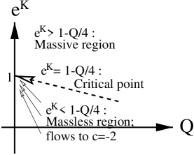
Figure 2: Phase diagram of the supersphere sigma model from the $Q$ state Potts model on the square lattice.

While the situation is not so familiar in two dimensions where most effort has been devoted to models based on unitary compact groups where the Mermin-Wagner-Coleman theorem prevents spontaneous symmetry breaking, it is well known in higher dimensions. There, one typically tackles exponents at the critical point in the $O(N)$ model with $(\vec{\Phi}^{2})^{2}$ coupling by studying the broken symmetry phase, i.e., the non-linear sigma model, in $d=2+\epsilon$, calculating the $\beta$ function in this phase, and identifying the critical point with the first zero of the $\beta$ function. The perturbative series thus obtained are only sensitive to the local structure of the group manifold, while the restoration of symmetry involves global properties.

To discuss things further, we consider the geometrical interpretation of the full sigma model. It is slightly more convenient to start from the non-scaled fermions, and consider the equivalent of Eq. (6) with the constraint $b(\phi)>0$ removed. To each site $i$ we assign an Ising variable $\epsilon_{i}=\pm 1$ which distinguishes between the two solutions (i.e., $b(\phi)>0$ and $b(\phi)<0$). One finds easily

$$Z_{\rm sigma} \equiv \int\prod_{i}{\rm d}\phi(i){\rm d}\eta_{1}(i){\rm d}\eta_{2}(i)\,\delta[\phi^{2}(i)+2a\eta_{1}(i)\eta_{2}(i)-1]\,\exp\left[-\frac{1}{a}\sum_{\langle ij\rangle}\left(\vec{u}(i)\cdot\vec{u}(j)-1\right)\right]$$

$$= \int\prod_{i}{\rm d}\eta_{1}(i){\rm d}\eta_{2}(i)\,\sum_{\{\epsilon_{i}\}}\exp\left[-{1\over a}\sum_{<ij>}(\epsilon_{i}\epsilon_{j}-1)\right]$$

$$\times\exp\left[\sum_{i,j}\eta_{1}(i)m_{ij}\eta_{2}(j)+\sum_{i}[\eta_{1}(i)\eta_{2}(i)(a+\epsilon_{i}\tilde{\epsilon}_{i}-m_{ii})-a\sum_{\langle ij\rangle}\epsilon_{i}\epsilon_{j}\eta_{1}(i)\eta_{2}(i)\eta_{1}(j)\eta_{2}(j)\right]$$

where we have defined $\tilde{\epsilon}_{i}=-\sum_{j\neq i}m_{ij}\epsilon_{j}$. For the region of broken symmetry, $a$ is negative, and thus the existence of domain walls with $\epsilon_{i}\epsilon_{j}=-1$ extremely unfavorable for small $|a|$. If we think of the $\epsilon_{i}$’s as Ising variables (essentially the c-number parts of the field $\phi$), we have a ferromagnetic Ising model coupled to the arboreal gas. A full geometrical interpretation is easily obtained by going over the steps of [7]. The $\eta$ terms again give an arboreal gas, but now each tree gets a more complicated weight

$$a\rightarrow a+\sum_{i{\rm\ in\ tree}}(\epsilon_{i}\tilde{\epsilon}_{i}-m_{ii})-a\sum_{\langle ij\rangle{\rm\ in\ tree}}(\epsilon_{i}\epsilon_{j}-1)$$ (14)

so now trees getting near or across domain walls have their weight modified.

As the lattice coupling is modified, a first sight analysis would say that generically in such a model, one will observe two transitions: an Ising transition where only the dynamics of the $\epsilon_{i}$ variables becomes critical, and an arboreal gas transition, where only the dynamics of the trees becomes critical. These transitions will occur for different values of $a$. Hence the critical point of the arboreal gas, i.e., the hemi-sphere lattice sigma model, will coincide in general with the critical point of the coupled system [Ising model + arboreal gas], i.e., the full lattice sigma model. Only an extraordinary coincidence could make the Ising and arboreal transitions merge, resulting in a higher order phase transition, and a situation where the critical points of the hemi-sphere and full sigma model are different, the latter being of higher order, and less stable.

This whole analysis may have to be taken with a grain of salt however. In particular, the arboreal gas is a model whose weights are extremely non-local, and the modification brought by coupling to the Ising variables might have strange consequences. Also, it is after all not clear how much of the conventional wisdom derived from models with positive Boltzmann weights will extend to models such as ours, where the physics is determined by balance of positive and negative contributions in addition to the usual energy/entropy balance. At this stage, numerical study seems the best way to clarify the situation.

3 Bethe equations at the antiferromagnetic point

The special value $a=-4$ identified above corresponds more precisely to the end point $Q\rightarrow 0$ of the antiferromagnetic critical line, which was identified by Baxter [17] as

$$\left({\rm e}^{K_{1}}+1\right)\left({\rm e}^{K_{2}}+1\right)=4-Q$$ (15)

(here $K_{1},K_{2}$ are the usual horizontal and vertical couplings). While the Potts model on the square lattice is not solvable for arbitrary couplings, it does become solvable on the line (15). The Bethe ansatz equations were written in the original paper by Baxter, and read

$$\left({\sinh(\lambda-i\gamma)\over\sinh(\lambda+i\gamma)}\right)^{N}=\prod_{\lambda^{\prime}}{\sinh{1\over 2}(\lambda-\lambda^{\prime}-2i\gamma)\over\sinh{1\over 2}(\lambda-\lambda^{\prime}+2i\gamma)}$$ (16)

where $N$ is the width of the cylinder in the transfer matrix (measured in terms of the Potts spins), the $\lambda$ are the usual spectral parameters determining the Bethe wave function, and we have parameterized $\sqrt{Q}=2\cos\gamma$, $\gamma\in\left[0,{\pi\over 2}\right]$. As discussed in details in [9] for the case $Q$ generic, the physics of the isotropic model $K_{1}=K_{2}$ can be studied more conveniently by considering a strongly anisotropic limit and the associated quantum hamiltonian for a chain of $2N$ spins $1/2$. The energy (in the relativistic scale) is then given by

$$E={\pi-2\gamma\over\pi}\sum_{\lambda}{2\sin 2\gamma\over\cosh 2\lambda-\cos 2\gamma}$$ (17)

We expect that the ground state is obtained by filling up the lines Im $\lambda={\pi\over 2}$ and Im $\lambda=-{\pi\over 2}$. If we restrict to solutions of the type $\lambda\equiv{i\pi\over 2}+\alpha$ and $\lambda\equiv-{i\pi\over 2}+\beta$, a system of two equations for the real parts $\alpha$ and $\beta$ can then we written. It can also be extended to string configurations centered on either line.

We now focus on the limit $\gamma\rightarrow{\pi\over 2}$. We set $\gamma={\pi\over 2}+\epsilon$, and scale the spectral parameters with $\epsilon$. The resulting system of equations reads (we use the same notations for the rescaled spectral parameters)

$$\left({\alpha-i\over\alpha+i}\right)^{N}=\prod{\alpha-\beta-2i\over\alpha+\beta+2i}$$

$$\left({\beta-i\over\beta+i}\right)^{N}=\prod{\beta-\alpha-2i\over\beta-\alpha+2i}$$ (18)

and the energy

$$E=-{4\over\pi}\sum{1\over 1+\alpha^{2}}+{1\over 1+\beta^{2}}$$ (19)

4 Critical properties at the antiferromagnetic point

4.1 First aspects

We now observe that setting $\alpha=\beta$ gives Bethe equations similar to the antiferromagnetic XXX chain, while there is an additional factor of $2$ in the definition of the energy. The sector symmetric in $\alpha$ and $\beta$ roots will lead to twice the central charge and critical exponents of the XXX chain, which are the ones of a free boson with coupling constant $g=1$, or an $SU(2)$ WZW model at level one (a similar feature was encountered in [5]. This is more than a coincidence, as will be discussed below).

This is not to say that all the excitations are of this type. Doubling the spectrum of the XXZ chain of course creates many gaps in the conformal towers, which have to be filled with other types of excitations in our system. But at least, we can derive quickly some results from this subset of the spectrum, which is now under control.

For the electric part of the spectrum, we then get the following result

$$c=2\times\left(1-{6e^{2}\over g}\right)=2-12e^{2}$$ (20)

The charge $e$ can be interpreted as giving a special weight $w$ to non-contractible loops. Following the detailed mappings of the Potts model on contours and vertex models, one finds $w=2\cos\pi e$. Since non-contractible loops come in pairs, we have $e$ defined modulo an integer. The $Q\rightarrow 0$ state Potts model itself corresponds to $e=e_{0}={1\over 2}$, for which $c=-1$, while the effective central charge is $c_{\rm eff}=2$.

Magnetic gaps read similarly

$$\Delta=2\times{gm^{2}\over 4}={m^{2}\over 2}$$ (21)

Here $m$ is the spin of the equivalent XXX chain. Since one solution of the equivalent XXX system corresponds to a pair of solutions of our system, $m={N\over 2}-[\hbox{number of pairs of solutions}]$ and $m={S^{z}\over 2}$, where $S^{z}$ is the spin in our initial system. Therefore

$$\Delta={(S^{z})^{2}\over 8}$$ (22)

where $S^{z}$ is an integer since we have an even number of spins.

One can see here that parity effects will likely occur. If $N$ is even, since we must also have an even number of upturned spins to make up pairs of Bethe roots in the “folding” of the equations, the result strictly speaking will only apply to $S^{z}$ even, including the ground state. Numerical study shows that in fact it holds for $S^{z}$ odd as well. If $N$ is odd on the other hand, since we must also have an even number of upturned spins to make up pairs of Bethe roots in the “folding” of the equations, the result strictly speaking will only apply to $S^{z}$ odd. Numerically, we have observed indeed that for $S^{z}$ even, including the ground state $S^{z}=0$, results for $N$ odd obey a different pattern. This will be discussed later, and we restrict for now to $N$ even.

The electric charges in the $S^{z}=0$ sector of the equivalent XXX chain are, for the untwisted case, integer, and give rise to the following gaps $\Delta=2\times{e^{2}\over 4g}={e^{2}\over 2}$. Combining all the excitations, we thus get exponents from a single free boson at $g={1\over 2}$, viz., $\Delta_{em}={1\over 2}\left(e\pm{S^{z}\over 2}\right)^{2}$, where $e,S^{z}$ are integers. This is intuitively satisfactory, as one expects the “arrows degrees of freedom” in the model to be described by a free boson in general. This free boson of course contributes only $c=1$ to the total central charge, so to get $c=2$ we need to invoke the presence of another theory with $c=1$.

To proceed, we consider the dynamics of the hole excitations over the ground state where the two lines $\hbox{Im }\lambda=\pm{\pi\over 2}$ are filled. We introduce the functions (notations are the same as in [18])

$$e_{n}(\alpha)={\alpha+in/2\over\alpha-in/2};~{}~{}~{}a_{n}(\alpha)={i\over 2\pi}{{\rm d}\over{\rm d}\alpha}\ln\left[e_{n}(\alpha)\right]$$ (23)

and the Fourier transform

$$\hat{f}(x)=\int{\rm d}\alpha\,{\rm e}^{i\alpha x}f(\alpha)$$ (24)

such that $\hat{a}_{n}(x)={\rm e}^{-n|x|/2}$. We take the logarithm of the Bethe equations [Eq. (18)] and introduce densities of particles ($\rho$) and holes ($\rho^{h}$) per unit length. The result in Fourier transforms reads

$$\hat{\rho}_{1}+\hat{\rho}_{1}^{h}=a_{2}-a_{4}\star\rho_{2}$$

$$\hat{\rho}_{2}+\hat{\rho}_{2}^{h}=a_{2}-a_{4}\star\rho_{1}$$ (25)

and is of the form $\hat{\rho}+\hat{\rho}^{h}=\hat{p}+K\hat{\rho}$. Physical equations (that is, equations where the right hand side depends on density of excitations) meanwhile read

$$\hat{\rho}_{1}+\hat{\rho}_{1}^{h}={1\over 2\cosh x}+{1\over 1-{\rm e}^{4|x|}}\hat{\rho}_{1}^{h}+{1\over 2\sinh 2x}\hat{\rho}_{2}^{h}$$

$$\hat{\rho}_{2}+\hat{\rho}_{2}^{h}={1\over 2\cosh x}+{1\over 2\sinh 2x}\hat{\rho}_{1}^{h}+{1\over 1-{\rm e}^{4|x|}}\hat{\rho}_{2}^{h}$$ (26)

Introducing the matrix $Z=(1-K)^{-1}$ one finds

$$Z=\left(\begin{array}[]{cc}{1\over 1-{\rm e}^{-4|x|}}&{-1\over 2\sinh 2x}\\ {-1\over 2\sinh 2x}&{1\over 1-{\rm e}^{-4|x|}}\end{array}\right)_{x=0}$$ (27)

Now in ordinary models such as those with $sl(n)$ symmetry, it is well known how to obtain analytically the spectrum of exponents by careful analysis of finite size scaling effects. The exponents are expressed as quadratic forms based on the matrix $Z$ and its inverse [19, 20]. We shall assume a bit naively that the same essentially is true here as well. All the elements of $Z$ diverge in the limit $x=0$, but if we keep $x$ small, $Z$ reads

$$Z=\left(\begin{array}[]{cc}{1\over 2}+{1\over 4\epsilon}&{-1\over 4\epsilon}\\ {-1\over 4\epsilon}&{1\over 2}+{1\over 4\epsilon}\end{array}\right)$$ (28)

which allows us to calculate the inverse matrix as $\epsilon\rightarrow 0$

$$Z^{-1}=\left(\begin{array}[]{cc}1&1\\ 1&1\end{array}\right)$$ (29)

We can now let $\epsilon\rightarrow 0$ to express the finite size scaling corrections and thus the gaps for $N$ even as [20]

$$x={1\over 4}\delta n^{t}Z^{-1}\delta n+d^{t}Zd$$ (30)

where $\delta n$ is the two-column vector $\left(\begin{array}[]{c}\delta n_{1}\\ \delta n_{2}\end{array}\right)$, $\delta n_{i}$ the change of solutions of the $i^{th}$ type. Similarly, $d$ is the two-column vector $\left(\begin{array}[]{c}d_{1}\\ d_{2}\end{array}\right)$, $d$ the number of particles backscattered from the left to the right of the Fermi sea. Therefore we find

$$\Delta+\bar{\Delta}={1\over 4}(\delta n_{1}+\delta n_{2})^{2}+0\times(\delta n_{1}-\delta n_{2})^{2}+{1\over 4}(d_{1}+d_{2})^{2}+\infty\times(d_{1}-d_{2})^{2}$$ (31)

The symmetric part of the spectrum $\delta n_{1}=\delta n_{2}=\delta n$ and $d_{1}=d_{2}=d$ gives $h+\bar{h}=(\delta n)^{2}+d^{2}$. We have checked numerically that this formula extends to the case $\delta n$ half odd integer, so the total XXX part of the spectrum reads $h+\bar{h}=e^{2}+{m^{2}\over 4}$, $e,m$ integers, or $h={1\over 8}(m+2e)^{2}$ and $\bar{h}={1\over 8}(m-2e)^{2}$. This corresponds to a free boson at the coupling $g=1/2$, i.e., symplectic fermions. It is useful to introduce now the determinants of the Laplacian on a torus with different types of boundary conditions, $\hbox{Det }\Delta_{ab}$; the subindices denote the boundary conditions ($P=$ periodic, $A=$ antiperiodic, or $F=$ free), with $b$ referring to the space direction (of length $N$) and $a$ to the imaginary time direction (of length $M$, with modular parameter $q={\rm e}^{-2\pi M/N}$) [21]:

$$\hbox{Det }\Delta_{AP} = {1\over\eta\bar{\eta}}\sum_{n,m}q^{(2n+1)^{2}/8}\bar{q}^{(2m+1)^{2}/8}$$

$$\hbox{Det }\Delta_{AA} = {1\over\eta\bar{\eta}}\sum_{n,m}q^{(2n)^{2}/8}\bar{q}^{(2m)^{2}/8}$$

$$\hbox{Det }\Delta_{PA} = {1\over\eta\bar{\eta}}\sum_{n,m}(-1)^{n}q^{(2n)^{2}/8}(-1)^{m}\bar{q}^{(2m)^{2}/8}$$ (32)

where $\eta=q^{1/24}\prod_{1}^{\infty}(1-q^{n})$ is Dedekind’s eta function. The generating function of XXX levels in the case $N$ even thus reproduces $\hbox{Det }\Delta_{AP}+\hbox{Det }\Delta_{PA}+\hbox{Det }\Delta_{AA}$.

Combined with this symplectic fermion part, we have an infinite degeneracy associated with the modes $d_{1}=d_{2}$. Presumably, this leads to a continuous spectrum of exponents on top of the symplectic fermion ones. Since on the other hand we know that the theory has $c=-1$ ($c_{\rm eff}=2$) while the symplectic fermion part identified so far has $c=-2$ ($c_{\rm eff}=1$) , it is very tempting at this stage to propose that the missing part of the spectrum consists simply in a non-compact boson. We now give a more direct argument for this.

4.2 Lessons from free boundary conditions and modular transformations

The partition function of the $Q=0$ Potts model on an annulus with free boundary conditions can be obtained in two steps, both based on previous works. The first step consists is expressing it as an alternate sum over generating functions of levels for type II representations of $U_{t}sl(2)$ (where $\sqrt{Q}=t+t^{-1}$, and we use the notation $t$ for the quantum deformation parameter to avoid confusion with $q$) [22] in the associated six-vertex or XXZ model (not to be confused with the XXX model which appears through its Bethe equations earlier in this paper as a subsector of the Potts model. The latter has $t=1$ while the former has $t=i$). The second step consists in identifying the generating function $K_{j}$ of levels for the type II representations. This step is not rigorous, and based on our understanding of the model at special points $\gamma={\pi\over n}$, $n>2$, together with arguments of continuity in $\gamma$ [10]. To make a long story short, one ends up with the following results.

The expression of $K_{j}$ as $Q\rightarrow 0$ is

$$K_{j}={q^{j(j+1)/2+1/24}\over P^{2}(q)}\left[1+2\sum_{n=1}^{\infty}q^{2n^{2}+n(2j+1)}-2\sum_{n=0}^{\infty}q^{2(n+1/2)^{2}+(n+1/2)(2j+1)}\right]$$ (33)

where $P(q)=\prod_{1}^{\infty}(1-q^{n})$, and $j$ is an integer (spin) label, $j=0,1,2\ldots$. The astute reader might wonder why this expression does not satisfy for instance $K_{0}-K_{1}+K_{2}-K_{3}\ldots=0$ which would naively result from the quantum group symmetry that mixes all spin $0$ and spin $1$ representations [22]. The reason is that the eigenvalues of the transfer matrix all go to zero as $Q\rightarrow 0$, and this transfer matrix cannot be rescaled in such a way that its elements remain all finite as $Q\rightarrow 0$. Alternatively, in a hamiltonian formulation, the ground state energy of the relativistic hamiltonian goes to $-\infty$ in the limit $Q\rightarrow 0$. In that limit, the $K_{j}$’s are obtained after an additional renormalization, and do not have to satisfy the quantum group induced coincidences any longer.

A little algebra shows that the generating function of levels (partition function in the conformal language) of the XXZ or six-vertex model on the annulus is

$$Z_{PF}^{\rm vertex}=\sum_{j=0}^{\infty}(2j+1)K_{j}={q^{1/24}\over P^{2}(q)}\sum_{N=0}^{\infty}q^{N(N+1)/2}$$ (34)

In the usual case of the critical $Q=0$ state Potts model, the equivalent of $K_{j}$ would be

$$\tilde{K}_{j}={q^{j(j-1)/2+2/24}\over P(q)}\left(1-q^{1+2j}\right)$$ (35)

(in that case one checks that $\tilde{K}_{0}-\tilde{K}_{1}+\tilde{K}_{2}-\tilde{K}_{3}\ldots=0$ indeed). The partition function of the vertex model would then be in that case

$$\tilde{Z}^{\rm vertex}_{PF}=4{q^{2/24}\over P(q)}\sum_{N=0}^{\infty}q^{N(N+1)/2}$$ (36)

It corresponds to the partition function of symplectic fermions on an annulus with antiperiodic boundary conditions in the time direction, $\hbox{det}\left(-\Delta_{AF}\right)$, and is as well a character of the $c=-2$ rational logarithmic theory [23]. The object $Z^{\rm vertex}_{PF}$ written as $Z^{\rm vertex}_{PF}=\tilde{Z}^{\rm vertex}_{PF}\times{1\over\eta}=\hbox{det}\left(-\Delta_{AF}\right)\times{1\over\eta}$ can thus be interpreted as arising from a theory made of symplectic fermions and a non-compact boson, with partition function ${1\over\eta}$.

The presence of the non-compact boson can be ascertained through a modular transformation. Writing $\tilde{Z}^{\rm vertex}_{PF}=2{\theta_{2}(q)\over\eta(q)}$, we see that modular transformations in the usual $Q=0$ critical Potts model do close, since

$$\theta_{2}(-1/\tau) = \sqrt{-i\tau}\theta_{4}(-1/\tau)$$

$$\theta_{4}(-1/\tau) = \sqrt{-i\tau}\theta_{2}(-1/\tau)$$

$$\eta(-1/\tau) = \sqrt{-i\tau}\eta(\tau)$$ (37)

In the antiferromagnetic case meanwhile we now generate a continuous spectrum, according to

$${1\over\eta(-1/\tau)}\propto\int{\rm d}\alpha\,{{\rm e}^{2i\pi\tau\alpha^{2}}\over\eta(\tau)}$$ (38)

As for the arboreal gas or (the properly defined limit of) the Potts model itself, the partition function is

$$Z^{\rm arboreal}_{PF}=\sum_{0}^{\infty}(-1)^{j}K_{j}={q^{1/24}\over P^{2}}\sum_{N=0}^{\infty}(2N+1)(-1)^{N}q^{N(N+1)/2}$$ (39)

This can be written, using the Jacobi identity, as

$$Z^{\rm arboreal}_{PF}=q^{1/24}P(q)$$ (40)

The corresponding object in the usual critical Potts model ($\tilde{Z}_{PF}$) would vanish identically. As before, $Z^{\rm arboreal}_{PF}$ can be interpreted as the partition function of symplectic fermions (here, fermions periodic on the annulus, and the zero mode subtracted) times the contribution from a non-compact boson, ${1\over\eta}$.

We thus see that the study of the model with free boundary conditions greatly strengthens the claim that the continuum limit of the model is made up of a symplectic fermion theory and a non-compact boson. This of course agrees with $c=-1$, $c_{\rm eff}=2$. Let us discuss this identification further.

4.3 The continuum limit of the $Q=0$ antiferromagnetic critical Potts model

The action corresponding to this continuum limit reads (Boltzmann weight ${\rm e}^{-S}$)

$$S\propto\int{\rm d}^{2}x\,\left[\left(\partial_{\mu}\phi\right)^{2}+2\partial_{\mu}\eta_{1}\partial_{\mu}\eta_{2}\right]$$ (41)

with the boson $\phi$ being non-compact. Now recall that the scaling limit of the arboreal gas, or the $Q=0$ Potts model in the Berker-Kadanoff phase, was identified with the $OSP(1/2)$ supersphere sigma model, whose action reads exactly like Eq. (41) with the additional constraint that $\phi^{2}+2\eta_{1}\eta_{2}=1$. To all appearances therefore, the critical point of the arboreal gas simply corresponds to a free $OSP(1/2)$ field theory, where the constraint has been forgotten, and the symmetry is realized linearly. This interpretation requires some further discussion. The sigma model in the massless Berker-Kadanoff (spontaneously broken symmetry) phase has action

$$S={1\over g}\int{\rm d}^{2}x\,\left[\left(\partial_{\mu}\phi\right)^{2}+2\partial_{\mu}\eta_{1}\partial_{\mu}\eta_{2}\right]$$ (42)

with $g$ a negative quantity. It thus looks as if the natural action for the theory without constraint should be Eq. (41) with a negative sign. While this has no importance for the fermions (the sign for them can be switched by a trivial relabeling) it is not so at all for the boson. While the model $S=+\int(\partial\phi)^{2}$ is well defined, the model with $S=-\int(\partial\phi)^{2}$ is naively rather ill defined! It is possible to argue however, that since the theory is not compactified, this sign does not really matter.

Start with the ‘proper’ free uncompactified boson, with action (we put numerical constants explicitly now)

$$S={1\over 2}\int{\rm d}^{2}x\,\partial_{\mu}\phi\partial_{\mu}\phi$$ (43)

and thus propagator $\langle\phi(z,\bar{z})\phi(0)\rangle=-{1\over 4\pi}\ln|z|^{2}$. The fact that $\phi$ is not compactified allows all powers of $\phi$ as fields, and hence by summation, all complex exponentials. However, since only normalizable states appear in the partition function (see [24, 25] for further discussion on this point), only imaginary exponentials will show up there. This is compatible with the result of the functional integration

$$Z={1\over\sqrt{Im\tau}}{1\over\eta\bar{\eta}}={1\over\eta\bar{\eta}}\int_{-\infty}^{\infty}(q\bar{q})^{\alpha^{2}/4}\,{\rm d}\alpha$$ (44)

Hence in a transfer matrix study of such a model, we would see essentially a continuous spectrum above the central charge $c=1$. Note how the presence of operators with arbitrarily negative dimension does not make the theory unstable, nor does it affect the ground state in the transfer matrix calculations.

If we admit that the “full operator content” is built out of fields ${\rm e}^{(a+ib)\phi}$ and derivatives, then a change of variables $\phi\rightarrow i\theta$ should leave it invariant. This means that full operator content can be built as well out of ${\rm e}^{(a+ib)\theta}$ and derivatives, where now $\theta$ has a propagator with the wrong sign, $\langle\theta(z,\bar{z})\theta(0)\rangle=-{1\over 4\pi}\ln|z|^{2}$. Normalizable states now correspond to real exponentials, and their contribution to the partition function gives exactly the same result as Eq. (44), which can therefore be considered as the partition function for the theory with action

$$S=-{1\over 2}\int{\rm d}^{2}x\,\partial_{\mu}\theta\partial_{\mu}\theta$$ (45)

In other words, we define the functional integral in the case of Eq. (45) by analytic continuation, and since the set of allowed fields is invariant under this continuation, the partition function is the same in both cases.

The fact that the critical point of the supersphere sigma model appears to be the free theory is a bit surprising. One would have expected instead the $OSP(1/2)$ symmetry to be restored in a non-trivial way, and the model maybe to coincide with the critical $O(n=-1)$ model of Nienhuis [26], discussed more thoroughly as an $OSP(1/2)$ model in Ref. [3]. The latter model however has central charge $c=-{3\over 5}$, and definitely is very different from the one we obtain. This difference might be related to the difference between the hemi-supersphere and the full supersphere sigma model. It might also be that some of the simplifications in the definition of the solvable $O(n)$ critical model in [26] (such as the definition of the Boltzmann weight) affect the physics in an unexpected way when $n$ is negative, with, as a result, less universality than expected.

5 Relation with $OSP(2/2)$ theories

5.1 $osp(2/2)$ integrable spin chain.

We now notice that the Bethe equations bear a strange similarity with equations written for a chain with $sl(2/1)$ symmetry. In particular, if we took a chain with alternating $3,\bar{3}$ representations ($N$ of either type), the equations would read, in the appropriate grading [27, 5],

$$\left({\alpha-2i\over\alpha+2i}\right)^{N}=\prod{\alpha-\beta-2i\over\alpha+\beta+2i}$$

$$\left({\beta-2i\over\beta+2i}\right)^{N}=\prod{\beta-\alpha-2i\over\beta-\alpha+2i}$$ (46)

More generally, the Bethe equations for alternating representations build with $n$-supersymmetric tensors and the conjugate would look like Eq. (46), but with the factor $2$ replaced by $2n$ on the left-hand side (source terms). Our equations seem to correspond to taking “quarter spin” representations (in $sl(2)$ inspired conventions, where the fundamental has spin $1/2$). This in fact has a meaning, thanks to the work [28] where it was shown that the Bethe equations for a chain built with the four-dimensional typical representation (and $L$ sites) read

$$\left({\alpha-i(2b+1)\over\alpha+i(2b+1)}\right)^{L}=\prod{\alpha-\beta-2i\over\alpha+\beta+2i}$$

$$\left({\alpha+i(2b-1)\over\alpha-i(2b-1)}\right)^{L}=\prod{\beta-\alpha-2i\over\beta-\alpha+2i}$$ (47)

where $b$ is the fermionic Dynkin number (denoted by $b_{2}$ in [28]). The fundamental of $sl(2/1)$ corresponds to $b=-1$, a degenerate case. The case $b=0$ meanwhile corresponds to the fundamental representation of $osp(2/2)$. Energy terms in this case can also be read from [28] and exactly match the term in the $Q=0$ Potts model case (after a rescaling of the Bethe parameters in [28]). We thus conclude that the Bethe equations and energy for the $Q=0$ antiferromagnetic Potts spin chain are identical with those for the integrable spin chain with $osp(2/2)$ symmetry built on the four-dimensional fundamental representation $[b=0,j=1/2]$.

Note that the length of the $osp(2/2)$ system in these equations, denoted $L$ in the Bethe equations, coincides with $N$, where the number of spin $1/2$ representations in the spin chain is $2N$. Hence the size of the Hilbert spaces on which the two systems are acting are identical, and equal to $2^{2N}=4^{N}$. Since the Bethe equations also coincide, this is a very strong indication that the spectra of the two systems are identical, even though one has to be careful with such statements, as Bethe spectra are not always complete in the superalgebra case.

5.2 Continuum limit of the $osp(2/2)$ integrable spin chain.

Now, as argued in [31], the integrable model based on the four-dimensional fundamental representation of $osp(2/2)$ sits inside the Goldstone phase of this model, and goes to the supersphere sigma model $OSP(2/2)/OSP(1/2)$ in the scaling limit. The latter model can be described [30] by the following action. Parameterize the $S^{1,2}$ supersphere as

$$\phi_{1} = \cos\phi\left(1-\eta_{1}\eta_{2}\right)$$

$$\phi_{2} = \sin\phi\left(1-\eta_{1}\eta_{2}\right)$$ (48)

such that $\phi_{1}^{2}+\phi_{2}^{2}+2\eta_{1}\eta_{2}=1$. The action is then

$$S={1\over g}\int{\rm d}^{2}x\,\left[\left(\partial_{\mu}\phi\right)^{2}(1-2\eta_{1}\eta_{2})+2\partial_{\mu}\eta_{1}\partial_{\mu}\eta_{2}-4\eta_{1}\eta_{2}\partial_{\mu}\eta_{1}\partial_{\mu}\eta_{2}\right]$$ (49)

where $\phi$ is compactified, $\phi\equiv\phi+2\pi$. The integrable chain corresponds to spontaneously broken symmetry, with the theory being free in the UV and massless in the IR, corresponding to a negative coupling constant $g$. Critical properties are described by the $g\rightarrow 0$ limit of Eq. (49). A rescaling and relabeling brings Eq. (49) into the form

$$S=\int{\rm d}^{2}x\,\left[-\left(\partial_{\mu}\phi\right)^{2}(1+2|g|\eta_{1}\eta_{2})+2\partial_{\mu}\eta_{1}\partial_{\mu}\eta_{2}+4|g|\eta_{1}\eta_{2}\partial_{\mu}\eta_{1}\partial_{\mu}\eta_{2}\right]$$ (50)

with now $\phi\equiv\phi+{2\pi\over\sqrt{|g|}}$. As $g\rightarrow 0$, we thus obtain a symplectic fermion and a non-compact boson, with the wrong sign of the metric. This is exactly the low-energy theory we had identified earlier for the $Q=0$ antiferromagnetic Potts model, thus confirming our picture.

Note that the presence of a continuous spectrum in this $osp(2/2)$ version of the problem has a physical origin in the fact that the symmetry is spontaneously broken, and thus correlation functions of order parameters have no algebraic decay (though have logarithmic behaviour). This feature was verified numerically in [31] where it was found that the scaling dimensions of $p$ leg polymer operators extracted through transfer matrix calculations vanish inside the entire Goldstone phase indeed.

As a final note we remark that the Bethe equations for the $osp(2/2)$ chain have been most often [32, 33] written in a different grading from the one we used. It is also interesting to compare the analysis of the low energy physics from the more standard point of view.

The usual Bethe equations are written as

$$\left({\alpha-i\over\alpha+i}\right)^{L} = \prod{\alpha-\beta-2i\over\alpha-\beta+2i}$$

$$\prod{\beta-\alpha-2i\over\beta-\alpha+2i} = \prod{\beta-\beta^{\prime}-4i\over\beta-\beta^{\prime}+4i}$$ (51)

with the energy

$$E={4\over\pi}\sum{1\over 1+\alpha^{2}}$$ (52)

(note the change of sign compared to the other Bethe ansatz). The relevant solutions for the low energy physics are: $\alpha$ two-strings centered on real $\beta$’s (denoted then by $y$), and real $\alpha$’s (which are not in complexes, denoted then by $z$). The corresponding Bethe equations are

$$\left({y-3i\over y+3i}{y+i\over y-i}\right)^{L} = \prod_{y^{\prime}}{y-y^{\prime}-4i\over y-y^{\prime}+4i}\prod_{z}{y-z-2i\over y-z+2i}$$

$$\left({z-i\over z+i}\right)^{N} = \prod_{y}{z-y-2i\over z-y+2i}$$ (53)

The ground state is filled with the complexes. Going to the continuum limit and using Fourier transform gives the following physical equations, if we call $\rho$ the density of complexes, $\sigma$ the density of real particles

$$\hat{\rho}+\hat{\rho}^{h} = {1\over 2\cosh x}-{{\rm e}^{-|2x|}\over 2\sinh 2|x|}\hat{\rho}^{h}+{1\over 2\sinh 2|x|}\hat{\sigma}$$

$$\hat{\sigma}+\hat{\sigma}^{h} = {1\over 2\cosh x}-{{\rm e}^{-2|x|}\over 2\sinh 2|x|}\hat{\sigma}+{1\over 2\sinh 2|x|}\hat{\rho}^{h}$$ (54)

These equations show that the chain has a relativistic limit (a feature peculiar to the value $b=0$ of the fundamental representation [18]). Moreover, the density equations coincide with those for the $Q\rightarrow 0$ antiferromagnetic Potts model discussed above: even though we have started from two different gradings, we end up with identical physical equations, a very strong indication that our approach is consistent [34] (note in particular that the quantum numbers of the excitations, being expressed naturally in terms of complexes and real holes, have different expressions in terms of the bare quantum numbers) and the results correct.

To finish the analysis of the $osp(2/2)$ system, the most useful quantity one can consider is the ‘equivalent spin’ defined by forming the combination $m\equiv b-3S^{z}$. The four states of the fundamental representation $b=0,S^{z}=\pm 1/2;S^{z}=0,b=\pm 1/2$ correspond respectively to the values $m=3/2,1/2,-1/2,-3/2$. On the other hand, according to the detailed lattice model derivation of the Bethe ansatz equations [33, 32],

$$m=b-3S^{z}=\#\beta-\#\alpha-{L\over 2}$$

The spectrum is expressed in terms of sums and differences of $\delta n_{c}^{h}$ and $\delta n_{r}$, where the subscripts $c,r$ indicate complexes and real particles respectively. One has

$$\delta n_{c}^{h}-\delta n_{r} = \delta n_{\beta}-\delta n_{\alpha}$$

$$\delta n_{c}^{h}+\delta n_{r} = \delta n_{\beta}-3\delta n_{\alpha}$$ (55)

We thus see that it is possible to change the value of the pseudospin $m$ without changing $\delta n_{c}^{h}+\delta n_{r}$, i.e., by exciting only the flat part of the spectrum. In other words, in the geometrical interpretation, the gaps for $p$ leg operators are all expected to vanish. This result agrees with predictions based on the Goldstone analysis of the $OSP(2/2)$ loop model, as well as numerical calculations [31], and we take the consistency of the different approaches as a justification of our use of the dressed charge formalism in these problems.

5.3 Explicit mapping between the two models

Even though we have found that the Bethe equations for the two models are identical, we do not exactly know how to map them onto each other. Clearly, one must combine pairs of neighbouring spin $1/2$ representations of the vertex model to make up four-dimensional representations of the $osp(2/2)$ algebra, but we are not sure how to implement this. Part of the difficulty comes from the highly singular nature of the Potts transfer matrix as $Q\rightarrow 0$.

It is interesting to notice however that as $t\rightarrow i$, the tensor product of two fundamental representations of $U_{t}sl(2)$, which decomposes as the sum of a one and a three dimensional representations like for $t=1$ when $t$ is generic, becomes indecomposable, and has the structure shown in Fig. 3, where $|u_{1}\rangle={\rm e}^{i\pi/4}|+-\rangle+{\rm e}^{-i\pi/4}|-+\rangle$ and $|u_{2}\rangle={\rm e}^{-i\pi/4}|+-\rangle+{\rm e}^{i\pi/4}|-+\rangle$, and the arrows indicate the action of the $U_{t}sl(2)$ generators:

$$S^{-} = t^{\sigma^{z}}\otimes\sigma^{-}+\sigma^{-}\otimes t^{-\sigma^{z}}$$

$$S^{+} = t^{\sigma^{z}}\otimes\sigma^{+}+\sigma^{+}\otimes t^{-\sigma^{z}}$$ (56)

Figure 3: Indecomposable representation $1/2^{\otimes 2}$ for $t=i$.

It turns out that, if one introduces the other generators

$$\tilde{S}^{-} = t^{-\sigma^{z}}\otimes\sigma^{-}+\sigma^{-}\otimes t^{\sigma^{z}}$$

$$\tilde{S}^{+} = t^{-\sigma^{z}}\otimes\sigma^{+}+\sigma^{+}\otimes t^{\sigma^{z}}$$ (57)

at $t=i$, together with the limits $\lim_{t\rightarrow i}{(S^{\pm})^{2}\over t+t^{-1}}$, one obtains the four-dimensional representation of $osp(2/2)$. This suggests a mechanism by which the symmetry of the lattice model must be enhanced at the critical point. One can in fact show by brute force that by concatenating pairs of spins $1/2$ into four degrees of freedom and carefully taking the $Q\rightarrow 0$ limit of the Boltzmann weights of the heterogeneous 6-vertex model equivalent to the critical antiferromagnetic $Q$ state Potts model, the $R$ matrix of the $osp(2/2)$ integrable vertex model in the fundamental ($[b=0,j=1/2]$) representation is indeed obtained. This will be discussed elsewhere.

Note of course that the $osp(2/2)$ integrable model can be reformulated as a loop model. In fact the whole Goldstone phase has been argued to be realized physically by taking a model made of a single dense loop where crossings are allowed. This can be obtained (and studied numerically) for instance by taking the usual [35] covering of the surrounding lattice of the square lattice with a single self avoiding loop, and then allowing self-crossings.

Figure 4: Mapping between forests and self-intersecting loops. Thin solid (resp. dashed) lines represent the lattice ${\cal L}$ (resp. the dual lattice ${\cal L}^{D}$). All edges of ${\cal L}^{D}$ penetrating the boundary of ${\cal L}$ are understood to join at a unique dual site situated on the infinite, exterior face of ${\cal L}$. Thick solid lines depict the forest (here with four component trees); thick dashed lines depict the (unique) dual tree. The grey (red online) solid line is a self-intersecting loop on the surrounding lattice (see text). It bounces off occupied edges (thick linestyle) on ${\cal L}$ and on ${\cal L}^{D}$, and self-intersects whenever a pair of intersecting direct and dual edges are both non-occupied.

It is well known that in the case where self-crossings are not allowed, the loop the hull of a spanning tree, hence giving rise to the well-known close relationship between the critical theory of dense polymers and that of spanning trees, both being related to symplectic fermions [12, 13]. This relationship can to some extent be generalized to the arboreal gas and the loop with self-crossings (see Fig. 4). Indeed, draw on the lattice ${\cal L}$ a spanning forest. Draw on the dual lattice ${\cal L}^{D}$ (which in particular contains a single site outside ${\cal L}$) a spanning tree. The resulting contour on the surrounding lattice is a single loop with a number of self-intersections equal to the number of trees on ${\cal L}$ plus one! So we have a sort of correspondence between a self-crossing loop and an arboreal gas, i.e., between a system with $osp(2/2)$ symmetry and the $Q\rightarrow 0$ antiferromagnetic Potts model. However, this is not a very satisfactory correspondence. In particular, because the tree on the dual lattice plays a crucial role in determining the loop configuration, there is no one to one correspondence between loop and forest. Also, giving a negative fugacity to trees corresponds to a negative weight for self-crossings of the loop, while the existence of the Goldstone phase was argued in [31] for positive weights only.

6 Conclusion

The most interesting conclusion is probably the emergence of a non-compact boson in the continuum limit of the critical antiferromagnetic Potts model at $Q=0$. Although it is difficult to demonstrate the existence of such a non-compact object based on any single analysis, the convergence of Bethe ansatz calculations, numerical calculations, and symmetry considerations, leaves very little doubt that the conclusion is correct. This is, to our knowledge (together with our earlier work on Goldstone phases [31], which as we saw is intimately related), the first time that a non-compact object appears in the continuum limit of a lattice model with a finite number of degrees of freedom (but ‘unphysical’ Boltzmann weights). In a subsequent work, we will see that this feature extends to the antiferromagnetic Potts model away from $Q=0$ [9].

We have also seen how this non-compact boson is part of a free $OSP(1/2)$ theory, which appears here as a critical point of the super (hemi-)sphere sigma model. The main question that remains unanswered in this study of the physics of models with supergroup symmetry is what happens to the ‘other’ (Nienhuis) critical $O(n=-1)$ model [26], and how this is related with a possible difference between the critical points in the hemi and full supersphere sigma models. We hope to get back to these questions soon.

To finish, we can clarify several remaining points. The first is the issue of what happens when the size of the lattice system $N$ is odd. As will be discussed in details for the general antiferromagnetic Potts model in [9], the spectrum in that case does not show any signs of non-compactness because the bosonic field $\phi$ appears to be twisted (and thus its properties independent of any compactification radius). By $OSP(1/2)$ symmetry, the fermionic field is also twisted, so the effective central charge in this sector is

$$c_{\rm eff}=c-24h_{\rm tw}^{\phi}-24h_{\rm tw}^{\eta}=-1-\frac{3}{2}+3=\frac{1}{2}$$ (58)

in agreement with numerical calculations [8, 9].

The second point is that numerical [8] as well as analytical arguments [9] suggest that the critical point is, in the Potts model point of view, approached from the Berker-Kadanoff phase (the broken symmetry phase) with a singularity in the free energy of the form

$$f\propto(a^{*}-a)\ln(a^{*}-a)\quad\mbox{as \ }a\uparrow a^{*}.$$ (59)

(We recall that $a^{*}=-4$ for the square lattice.) Using hyperscaling, this corresponds to a perturbation of the critical point by a field of vanishing dimension. There are of course plenty of such fields in the non-compact boson theory. We speculate that the scaling limit near and below $a^{*}$ could be described by the simple Landau-Ginzburg theory

$$S=\int d^{2}x\left[(\partial_{\mu}\phi)^{2}+2\partial_{\mu}\eta_{1}\partial_{\mu}\eta_{2}\right]+(a^{*}-a)\left(\phi^{2}+2\eta_{1}\eta_{2}-1\right)$$ (60)

for which the logarithm in $f$ [see Eq. (59)] follows as well.

	$a$	$L=6$	$L=8$	$L=10$	$L=12$	$L=14$
$x_{1}$:	0	0.0000	0.0000	0.0000	0.0000	0.0000
	-1	-0.0859	-0.0792	-0.0747	-0.0714
	-2	-0.1092	-0.0992	-0.0925	-0.0877
	-3	-0.1168	-0.1079	-0.1003	-0.0947
	-4	0.0000	0.0000	0.0000	0.0000	0.0000
$x_{2}$:	0	0.7492	0.7498	0.7499	0.7500
	-1	0.5823	0.5975	0.6075	0.6146
	-2	0.5216	0.5492	0.5663	0.5781
	-3	0.4936	0.5253	0.5464	0.5609
	-4	0.5466	0.5691	0.5830	0.5927
$x_{3}$:	0	1.9671	1.9894	1.9958	1.9980	1.9989
	-1		1.6959	1.7213	1.7384
	-2	1.4930	1.5727	1.6201	1.6514
	-3	1.4050	1.5062	1.5667	1.6065
	-4	1.5268	1.6157	1.6621	1.6907	1.7105

Table 1: Scaling exponents $x_{k}=2h_{k}$ describing the probability $P(r)\sim r^{-2x_{k}}$ that $k$ distinct trees come close in points $0$ and $r$. The data is obtained by fitting transfer matrix results in the random-cluster picture, on periodic square-lattice cylinders of widths $L$ and $L-2$. Note the strong finite-size dependence for tree fugacity $a\neq 0$. For $a=0$ the exact result is $x_{k}=(k^{2}-1)/4$ [12].

The last point concerns the physical interpretation of our results. This of course has to be taken with a bit of care, as our model involves negative Boltzmann weights. But the image we have is that in the region $a^{*}<a\leq 0$, the partition function is dominated by configurations where a single infinite tree covers a finite fraction of the lattice—this fraction is unity as $a\rightarrow 0$, and remains finite in the whole phase $a^{*}<a<0$, the rest of the lattice being covered by trees of finite size. Tree exponents are the same as in the limit $a\rightarrow 0$, as can be checked numerically in Table 1. In particular, the fact that the one-tree exponent remains equal to zero guarantees that there is an infinite tree, and that its fractal dimension is equal to two. At $a=a^{*}$, we have coexistence of two phases, one with an infinite tree of finite density, the other with only finite trees. As $a=a^{*}$ is crossed, the derivative of the free energy with respect to $a$ is discontinuous [8], implying that the average number of trees per lattice site, and thus the average size of finite trees, experiences a discontinuity. In the phase $a<a^{*}$ (like in the phase $a>0$), there are only finite trees, of typical linear size given by the finite correlation length. The point $a=a^{*}$ is actually a first-order critical point, that is a point where a first and second order phase transition coincide [8]. At such a point, some correlations still decay algebraically, while some of the thermodynamic properties have discontinuities. The latter translate into operators of vanishing dimensions, for which we expect an infinite multiplicity. The simplest formalism to encompass this multiplicity is a non-compact boson, in agreement with what was found previously.

We conclude with a side remark. The fermionic representation of the arboreal gas model, instead of being used to argue for the presence of an $OSP(1/2)$ symmetry, can be used to get yet another representation, this time in terms of a loop model. For this, go back to the initial path integral (3) written in terms of fermions $\eta_{1},\eta_{2}$ only

$$\exp\left[(4+t)\sum_{i}\eta_{1}(i)\eta_{2}(i)-\sum_{\langle ij\rangle}(\eta_{1}(i)\eta_{2}(j)+\eta_{1}(j)\eta_{2}(i))-t\sum_{\langle ij\rangle}\eta_{1}(i)\eta_{2}(i)\eta_{1}(j)\eta_{2}(j)\right]$$ (61)

Simply expand the exponent, and contract the fermions. This is like the standard high temperature expansion for the Nienhuis $O(n)$ model . It gives rise to a sum over non-intersecting loops, with weight $-2$ per loop (like in the $O(n=-2)$ model), plus non-overlapping monomers with weight $4+a$, and dimers (which can be considered as degenerate length-two loops) with weight $-a$. The critical point $a=-4$ means monomers disappear, dimers have weight $4$. We are not sure why this model should be critical—note the dimers seem to encourage swelling of the loops, instead of self attraction as one would expect to get to a tricritical point—and this direction certainly deserves further study. Note that a critical point with $c=-1$ has been identified in a modified version of the $O(n=-2)$ model in Ref. [36].

Acknowledgments: This work was supported by the Department of Energy (HS). We thank F. David and A. Sokal for discussions.

Appendix A Bethe equations

The standard integrable model based on the $sl(2/1)=osp(2/2)$ superalgebra is the Perk Schultz model. It uses the fundamental representation of dimension 3, and leads to the Bethe ansatz equations (for a review see [37])

$$\left({\alpha-2i\over\alpha+2i}\right)^{N}=\prod{\alpha-\beta-2i\over\alpha-\beta+2i}$$

$$\prod{\beta-\alpha-2i\over\beta-\alpha+2i}=\prod{\beta-\beta^{\prime}-4i\over\beta-\beta^{\prime}+4i}$$ (62)

Algebraically, these equations correspond to treating the fundamental representation of $sl(2/1)$ as a non-typical fermionic representation with parameters $[b,j]=[-1/2,1/2]$, of dimension 3 instead of 4. One could as well consider a model based on higher spin representations $[b,j]=[-j,j]$ obtained by taking the fully supersymmetric component in the product of $n=2j$ fundamental representations. The equations would read as Eq. (62) but on the left-hand side the factor $2$ would be replaced by $2n$.

More generally, for the four-dimensional typical representations $[b,j=1/2]$, the Bethe equations generalizing Eq. (62) read [38, 39, 40]

$$\left({\alpha+i(2b-1)\over\alpha-i(2b-1)}\right)^{N}=\prod{\alpha-\beta-2i\over\alpha-\beta+2i}$$

$$\prod{\beta-\alpha-2i\over\beta-\alpha+2i}=\prod{\beta-\beta^{\prime}-4i\over\beta-\beta^{\prime}+4i}$$ (63)

In particular, the case $b=0$ is similar to Eq. (62) but on the left-hand side the factor $2$ is replaced by $1$ corresponding roughly to taking a ‘quarter spin’.

The second type of Bethe ansatz for the Perk Schultz model is obtained when associating the fundamental representation to the bosonic root of the distinguished Dynkin diagram instead. One obtains then the so called Sutherland’s equations

$$1=\prod{\alpha-\beta-2i\over\alpha-\beta+2i}$$

$$\left({\beta-2i\over\beta+2i}\right)^{N}\prod{\beta-\alpha-2i\over\beta-\alpha+2i}=\prod{\beta-\beta^{\prime}-4i\over\beta-\beta^{\prime}+4i}$$ (64)

Finally, it is also possible to write a Bethe ansatz based on the alternative Dynkin diagram, where both roots are fermionic

$$1=\prod{\alpha-\beta-2i\over\alpha-\beta+2i}$$

$$\left({\beta-2i\over\beta+2i}\right)^{N}=\prod{\beta-\alpha-2i\over\beta-\alpha+2i}$$ (65)

In this ansatz, equations for a mix of the fundamental and its conjugate are particularly elegant [27]:

$$\left({\alpha-2i\over\alpha+2i}\right)^{N}=\prod{\alpha-\beta-2i\over\alpha-\beta+2i}$$

$$\left({\beta-2i\over\beta+2i}\right)^{N}=\prod{\beta-\alpha-2i\over\beta-\alpha+2i}$$ (66)

As for the model based on the four-dimensional representation, its equations are given in the text as Eq. (47) and correspond once again to taking a ‘quarter spin’.

References

- [1] M. Zirnbauer, Conformal field theory of the integer quantum Hall plateau transition, hep-th/9905054.
- [2] I. A. Gruzberg, A. W. W. Ludwig and N. Read, Phys. Rev. Lett. 82, 4524 (1999).
- [3] N. Read and H. Saleur, Nucl. Phys. B 613, 409 (2001).
- [4] V. Gurarie and A. W. W. Ludwig, Conformal field theory at central charge and two-dimensional critical systems with quenched disorder, hep-th/0409105.
- [5] F. Essler, H. Frahm and H. Saleur, The continuum limit of the integrable spin chain with alternating representations, cond-mat/0501197.
- [6] R. M. Gade, J. Phys. A 32, 7071 (1999).
- [7] S. Caracciolo, J. L. Jacobsen, H. Saleur, A. D. Sokal and A. Sportiello, Phys. Rev. Lett. 93, 080601 (2004).
- [8] J. L. Jacobsen, J. Salas and A. D. Sokal, Spanning forests and the -state Potts model in the limit , cond-mat/0401026.
- [9] J. L. Jacobsen and H. Saleur, in preparation.
- [10] H. Saleur, Nucl. Phys. B 360, 219 (1991).
- [11] R. J. Baxter, J. Phys. C 6, L445 (1973).
- [12] B. Duplantier and H. Saleur, Nucl. Phys. B 290, 291 (1987).
- [13] B. Duplantier and F. David, J. Stat. Phys. 51, 327 (1988).
- [14] H. Saleur, Nucl. Phys. B 382, 486 (1992).
- [15] R. J. Baxter, H. N. V. Temperley and S. E. Ashley, Proc. Roy. Soc. London A 358, 535 (1978).
- [16] D. Mouhanna, Autour des systèmes classiques magnétiques frustrés, thèse d’habilitation, Université Pierre et Marie Curie, Paris VI.
- [17] R. J. Baxter, Proc. Roy. Soc. London A 383, 43 (1982).
- [18] H. Saleur, Nucl. Phys. B 578, 552 (2000).
- [19] J. Suzuki, J. Phys. A 21, L1175 (1988).
- [20] H. de Vega and E. Lopes, Nucl. Phys. B 362, 261 (1991).
- [21] P. Di Francesco, P. Mathieu and D. Sénéchal, “Conformal field theory” (Springer Verlag, New York, 1997).
- [22] V. Pasquier and H. Saleur, Nucl. Phys. B 330, 523 (1990).
- [23] A. Bredthauer and M. Flohr, Nucl. Phys. B 639, 450 (2002).
- [24] K. Gawedzki, Non-compact WZW conformal field theories, hep-th/911076.
- [25] H. Saleur, in preparation.
- [26] B. Nienhuis, J. Stat. Phys. 34, 731 (1984).
- [27] J. Links and A. Foerster, J. Phys. A 32, 147 (1999).
- [28] M. Pfannmüller and H. Frahm, J. Phys. A 30, L543 (1997).
- [29] L. Mezincescu, R. Nepomechie, P. K. Townsend and A. Tsvelik, Nucl. Phys. B 406, 681 (1993).
- [30] B. Wehefritz-Kaufmann and H. Saleur, Nucl. Phys. B 628, 407 (2002).
- [31] J. L. Jacobsen, N. Read and H. Saleur, Phys. Rev. Lett. 90, 090601 (2003).
- [32] M. J. Martins and P. B. Ramos, J. Phys. A 28, L525 (1995).
- [33] P. B. Ramos and M. J. Martins, Nucl. Phys. B 500, 579 (1997).
- [34] F. H. L. Essler, V. E. Korepin and K. Schoutens, Int. J. Mod. Phys. B 8, 3205 (1994).
- [35] R. J. Baxter, Exactly solved models in statistical mechanics (Academic Press, London, 1982).
- [36] H. W. Blöte and B. Nienhuis, J. Phys. A 22, 1415 (1989).
- [37] F. Essler and V. Korepin, Phys. Rev. B 46, 9147 (1992).
- [38] Z. Maassarani, J. Phys. A 28, 1305 (1995).
- [39] M. P. Pfannmüller and H. Frahm, Nucl. Phys. B 479, 575 (1996).
- [40] A. J. Bracken, M. D. Gould, J. R. Links and Y. Z. Zhang, Phys. Rev. Lett. 74, 2768 (1995).