Statistical Mechanical Development of a Sparse Bayesian Classifier

Abstract

The demand for extracting rules from high dimensional real world data is increasing in various fields. However, the possible redundancy of such data sometimes makes it difficult to obtain a good generalization ability for novel samples. To resolve this problem, we provide a scheme that reduces the effective dimensions of data by pruning redundant components for bicategorical classification based on the Bayesian framework. First, the potential of the proposed method is confirmed in ideal situations using the replica method. Unfortunately, performing the scheme exactly is computationally difficult. So, we next develop a tractable approximation algorithm, which turns out to offer nearly optimal performance in ideal cases when the system size is large. Finally, the efficacy of the developed classifier is experimentally examined for a real world problem of colon cancer classification, which shows that the developed method can be practically useful.

1 Introduction

In recent years, the demand for methods to extract rules from high dimensional data is increasing in the research fields of machine learning and artificial intelligence, in particular, those concerning bioinformatics. One of the most elemental and important problems of rule extraction is bicategorical classification based on a given data set [1]. In a general scenario, the purpose of this task is to extract a certain relation between the input $\bm{x}\in\mathcal{R}^{N}$, which is a high dimensional vector, and the binary output $y\in\{+1,-1\}$, which represents a categorical label, from a training data set $D^{M}=\{(\bm{x}^{1},y^{1}),\dots,(\bm{x}^{\mu},y^{\mu}),\dots(\bm{x}^{M},y^{M})\}$ of $M(=1,2,\dots)$ examples.

The Bayesian framework offers a useful guideline for this task. Let us assume that the relation can be represented by a probabilistic model defined by a conditional probability $P(y|\bm{x},\bm{w})$, where $\bm{w}$ stands for a set of adjustable parameters of the model. Under this assumption, it can be shown that for an input $\bm{x}_{M+1}$, the Bayesian classification

$$\hat{y}^{M+1}=\mathop{\rm argmax}_{y^{M+1}}P(y^{M+1}|\bm{x}^{M+1},D^{M})$$ (1)

minimizes the probability of misclassification after the training set $D^{M}$ is observed [2]. Here $P(y^{M+1}|\bm{x}^{M+1},D^{M})=\int d\bm{w}P(y^{M+1}|\bm{x}^{M+1},\bm{w})P(\bm{w}|D^{M})$ is termed the predictive probability, and the posterior distribution $P(\bm{w}|D^{M})$ is represented by the Bayes formula

$$P(\bm{w}|D^{M})=\dfrac{P(\bm{w})P(D^{M}|\bm{w})}{\int d\bm{w}P(\bm{w})P(D^{M}|\bm{w})}=\dfrac{P(\bm{w})\prod_{\mu=1}^{M}P(y^{\mu}|\bm{x}^{\mu},\bm{w})}{\int d\bm{w}P(\bm{w})\prod_{\mu=1}^{M}P(y^{\mu}|\bm{x}^{\mu},\bm{w})},$$ (2)

using the traning data $D^{M}$ and a certain prior distribution $P(\bm{w})$.

However, even this approach sometimes does not provide a satisfactory result for real world problems. A major cause of difficulty is the redundancy that exists in real world data. For example, let us consider a classification problem of DNA microarray data, which is a standard problem of bioinformatics. In such problems, while the size of available data sets is less than one hundred, each piece of data is typically composed of several thousand components, the causality or relation amongst which is not known in advance  [3]. Simple methods that handle all the components usually overfit the training data, which results in quite a low classification performance for novel samples even when the Bayesian scheme of eq. (1) is performed. Therefore, when dealing with real world data, not only is the classification scheme itself very important but it is also important to reduce the effective dimensions, assessing the relevance of each component.

The purpose of this paper is to develop a scheme to improve the performance of the Bayesian classifier, introducing a mechanism for eliminating irrelevant components. The idea of the method is simple: in order to assess the relevance of each component of data, we introduce a discrete pruning parameter $c_{l}\in\{0,1\}$ for each component $x_{l}$, and classify $(c_{l}x_{l})$ instead of $\bm{x}=(x_{l})$ itself. Components for which $c_{l}=0$ are assigned are ignored in the classification. Assuming an appropriate prior for $\bm{c}=(c_{l})$ that controls the number of ignored components, we can introduce a mechanism to reduce the effective dimensions in the Bayesian classification (eq. (1)), which is expected to lead to an improvement of the classification performance.

In the literature, such pruning parameters have already been proposed in the research of perceptron learning [4] and linear regression problems [5]. However, as far as the authors know, the potential of this method has not been fully examined, nor have practically tractable algorithms been proposed for evaluating the Bayesian classification of eq. (1), which is computationally difficult in general. We will show that our scheme offers optimal performance in ideal situations and we provide a tractable algorithm that achieves a nearly optimal performance in such cases. For simplicity, we will here focus on a classifier of linear separation type, however, the developed method can be extended to non-linear classifiers, such as those based on the kernel method [6].

This paper is organized as follows. In the next section, section 2, we present details of the classifier we are focusing on. In section 3, the performance of the classifier is evaluated by the replica method to clarify the potential of the proposed strategy. We show that the scheme minimizes the probability of misclassification for novel data when the data includes redundant components in a certain manner. However, performing the scheme exactly is computationally difficult. In order to resolve this difficulty, we develop a tractable algorithm in section 4. We show analytically that a nearly optimal performance, predicted by replica analysis, is obtained by the algorithm in ideal cases. In section 5, the efficacy for a real world problem of colon cancer classification is examined, demonstrating that the developed scheme is competitive practically. The final section, section 6, is devoted to a summary.

2 Sparse Bayesian Classifier

The classifier that we will focus on is provided by a conditional probability of perceptron type  [7]

$$P(y|\bm{x},\bm{w},\bm{c})=f\left(\frac{y}{\sqrt{N}}\sum_{l=1}^{N}c_{l}w_{l}x_{l}\right),$$ (3)

where $c_{l}\in\{0,1\}$ is the pruning parameter and the activation function $f(u)$ satisfies $f(u)\geq 0$ and $f(u)+f(-u)=1$ for $\forall{u}\in\mathcal{R}$. To introduce the pruning effect, we also use

$$P(\bm{w},\bm{c})={\cal V}^{-1}{e^{-\sum_{l=1}^{N}(1-c_{l})\frac{w_{l}^{2}}{2}}\delta\left(\sum_{l=1}^{N}c_{l}-NC\right)\delta\left(\sum_{l=1}^{N}c_{l}w_{l}^{2}-NC\right)},$$ (4)

as the prior probability of the parameters $\bm{w}$ and $\bm{c}$, where $0\leq C\leq 1$ is a hyper parameter that controls the ratio of the effective dimensions. The factor $e^{-\sum_{l=1}^{N}(1-c_{l})\frac{w_{l}^{2}}{2}}$ is included to make the normalization constant ${\cal V}=\int d\bm{w}\sum_{\bm{c}}e^{-\sum_{l=1}^{N}(1-c_{l})\frac{w_{l}^{2}}{2}}\delta\left(\sum_{l=1}^{N}c_{l}-NC\right)\delta\left(\sum_{l=1}^{N}c_{l}w_{l}^{2}-NC\right)$ finite. As this microcanonical prior enforces the probability to vanish unless the pruning parameters $c_{i}\in\{0,1\}$ satisfy the constraint $\sum_{l=1}^{N}c_{l}=NC$, each specific parameter choice ignores certain $N(1-C)$ components of $\bm{x}$ for classification. These yield the posterior distribution $P(\bm{w},\bm{c}|D^{M})$ via the Bayes formula

$$P(\bm{w},\bm{c}|D^{M})=\dfrac{P(\bm{w},\bm{c})\prod_{\mu=1}^{M}P(y^{\mu}|\bm{x}^{\mu},\bm{w},\bm{c})}{\int d\bm{w}\sum_{\bm{c}}P(\bm{w},\bm{c})\prod_{\mu=1}^{M}P(y^{\mu}|\bm{x}^{\mu},\bm{w},\bm{c})},$$ (5)

which defines the Bayesian classifier as

$$\hat{y}^{M+1}=\mathop{\rm argmax}_{y^{M+1}}\int d\bm{w}\sum_{\bm{c}}f\left(\dfrac{y^{M+1}}{\sqrt{N}}\sum_{l=1}^{N}c_{l}w_{l}x^{M+1}_{l}\right)P(\bm{w},\bm{c}|D^{M}).$$ (6)

The pruning vector $\bm{c}$ eliminates irrelevant dimensions of data, which makes $\bm{x}$ sparse. Therefore, we term the classification scheme represented in eq. (6) the sparse Bayesian classifier (SBC).

3 Replica analysis

To evaluate the ability of the SBC, let us assume the following teacher-student scenario [7]. In this scenario, a “teacher” classifier is selected from a certain distribution $P_{\rm t}(\bm{w}_{o})$. For each of $M$ inputs $\bm{x}^{1},\bm{x}^{2},\ldots,\bm{x}^{M}$ which are independently generated from an identical distribution $P_{\rm in}(\bm{x})$, the teacher provides a classification label $y=\pm 1$ following the conditional probability $P(y|\bm{x},\bm{w}_{o})=f\left(\frac{y}{\sqrt{N}}\sum_{l=1}^{N}w_{ol}x_{l}\right)$, which constitutes the training data set $D^{M}$. Then, the performance of the SBC, which plays the role of “student” in this scenario, can be measured by the generalization error, which is defined as the probability of misclassification for a test input generated from $P_{\rm in}(\bm{x})$.

To represent a situation where certain dimensions are not relevant for the classification label, let us assume that the teacher distribution is provided as

$$P_{\rm t}(\bm{w}_{o})=\prod_{l=1}^{N}\left[(1-C_{\rm t})\delta(w_{ol})+C_{\rm t}\frac{e^{-\frac{w_{ol}^{2}}{2}}}{\sqrt{2\pi}}\right],$$ (7)

where $C_{\rm t}$ is the ratio of the relevant dimensions that the student does not know. For simplicity, we further assume that the inputs are generated from a spherical distribution $P_{\rm in}(\bm{x})=P_{\rm sph}(\bm{x})\propto\delta\left(|\bm{x}|^{2}-N\right)$, which guarantees that the correlation of $c_{l}w_{l}$ between different components is sufficiently weak when the parameters $\bm{w}$ and $\bm{c}$ are generated from the posterior $P(\bm{w},\bm{c}|D^{M})$. As a hard constraint, $\sum_{l=1}^{N}c_{l}w_{l}^{2}=\sum_{l=1}^{N}(c_{l}w_{l})^{2}=NC$ is introduced by the microcanonical prior of eq. (4). This implies that one can approximate the stability $\Delta=\frac{y}{\sqrt{N}}\sum_{l=1}^{N}c_{l}w_{l}x_{l}$ as

$$\Delta\simeq\sqrt{C-Q}u+\left\langle\Delta\right\rangle,$$ (8)

using a Gaussian random variable $u\sim{\cal N}(0,1)$, where $\left\langle\cdots\right\rangle=\int d\bm{w}\sum_{\bm{c}}P(\bm{w},\bm{c}|D^{M})(\cdots)$ and $Q=\frac{1}{N}\sum_{l=1}^{N}\left\langle c_{l}w_{l}\right\rangle^{2}$. This makes it possible to evaluate eq. (6) as

$$\hat{y}^{M+1} ={\rm sign}\left(\int Duf\left(\sqrt{C-Q}u+\left\langle\Delta\right\rangle\right)-\frac{1}{2}\right),$$ (9)

where ${\rm sign}(x)=\frac{x}{|x|}$ for $x\neq 0$, and $Du=\frac{du}{\sqrt{2\pi}}e^{-\frac{u^{2}}{2}}$. Further, one can also deal with the average stability $\left\langle\Delta\right\rangle$ and the teacher’s stability $\Delta^{o}=\frac{y}{\sqrt{N}}\sum_{l=1}^{N}w_{ol}x_{l}$ as Gaussian random variables, the variances and covariance of which are given as

$$\overline{(\Delta^{o})^{2}}=\frac{\bm{w}_{o}\cdot\bm{w}_{o}}{N}\simeq C_{\rm t},\quad\overline{\Delta^{o}\left\langle\Delta\right\rangle}=R,\quad\overline{\left\langle\Delta\right\rangle^{2}}=Q,$$ (10)

using $\overline{x_{i}x_{j}}=\delta_{ij}$ where $\overline{\cdots}=\int d\bm{x}P_{\rm sph}(\bm{x})(\cdots)$ and $R=\frac{1}{N}\sum_{l=1}^{N}w_{ol}\left\langle c_{l}w_{l}\right\rangle$. This, in conjunction with the symmetry of $y=\pm 1$ in the current system, indicates that the generalization error of the SBC can be evaluated as

$$\epsilon^{\rm SBC}_{g}=2\int Dz\left(1-\int Dvf\left(\sqrt{C_{\rm t}-\frac{R^{2}}{Q}}v+\frac{R}{\sqrt{Q}}z\right)\right)\Theta\left(\int Duf\left(\sqrt{C-Q}u+\sqrt{Q}z\right)-\frac{1}{2}\right),$$ (11)

where $\Theta(x)=1$ for $x>0$ and $0$ otherwise, using the macroscopic variables $R$ and $Q$, which can be assessed by the replica method [8, 9].

To assess $R$ and $Q$, we evaluate the average of the $n(=1,2,\ldots)$-th power of the partition function

$$Z(D^{M}) =\int d\bm{w}\sum_{\bm{c}}P(\bm{w},\bm{c})\prod_{\mu=1}^{M}P(y^{\mu}|\bm{w},\bm{c},\bm{x}^{\mu})$$

$$=\int d\bm{w}\sum_{\bm{c}}\prod_{\mu=1}^{M}f\left(\frac{y^{\mu}}{\sqrt{N}}\sum_{l}c_{l}w_{l}x^{\mu}_{l}\right){\cal V}^{-1}e^{-\sum_{l=1}^{N}\frac{1}{2}(1-c_{l})w_{l}^{2}}\delta\left(\sum_{l=1}^{N}c_{l}w_{l}^{2}-CN\right)\delta\left(\sum_{l=1}^{N}c_{l}-CN\right)$$ (12)

with respect to the training data set $D^{M}$. The analytical continuation from $n=1,2,\ldots$ to $n\in\mathcal{R}$ under the replica symmetric (RS) ansatz provides the expression for the RS free energy:

$$\frac{1}{N}{\left[\ln Z(D^{M})\right]_{D^{M},\bm{w}_{o}}}=\frac{1}{N}\lim_{n\to 0}\frac{\partial\ln\left[Z^{n}(D^{M})\right]_{D^{M},\bm{w}_{o}}}{\partial n}$$ (13)

$$=\mathop{\rm Ext}_{R,Q,\hat{R},\hat{Q},F,\lambda}\left[2\alpha\int Dz\int Dvf\left(\sqrt{C_{\rm t}-\frac{R^{2}}{Q}}v+\frac{R}{\sqrt{Q}}z\right)\ln\left(\int Duf\left(\sqrt{C-Q}u+\sqrt{Q}z\right)\right)\right.$$ (14)

$$-\hat{R}R+\frac{1}{2}{\hat{Q}Q}+\frac{1}{2}FC-\lambda C$$ (15)

$$+\left.\left\langle\int Dz\ln\left[1+\frac{1}{\sqrt{F+\hat{Q}}}\exp\left[\lambda+\frac{\left(\sqrt{\hat{Q}}z+\hat{R}w_{o}\right)^{2}}{2(F+\hat{Q})}\right]\right]\right\rangle_{w_{o}}\right]-\frac{1}{N}\ln{\cal V},$$ (16)

where $\left[\cdots\right]_{D^{M},\bm{w}_{o}}$ denotes the average over the training set $D^{M}$ and the teacher distribution of eq. (7), $\mathop{\rm Ext}_{x}(\cdots)$ denotes extremization of $\cdots$ with respect to $x$, which determines $R$ and $Q$, and $\alpha=M/N$ and $\left\langle\cdots\right\rangle_{w_{o}}=\int dw_{o}\left((1-C_{\rm t})\delta(w_{o})+C_{\rm t}\frac{e^{-\frac{w_{o}^{2}}{2}}}{\sqrt{2\pi}}\right)(\cdots)$.

Figure 1: Generalization error versus $C$ for (a) the SBC and (b) Gibbs learning ($\alpha=1,\kappa=0.05$).

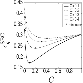
The generalization error $\epsilon^{\rm SBC}_{g}$ can be evaluated from eq. (11) using $R$ and $Q$ obtained via the extremization problem of eq. (16), which is plotted in fig. 1 (a) as a function of the hyper parameter $C$ in the case of

$$f(u)=f(u;\kappa)=\kappa+(1-2\kappa)\Theta(u),$$ (17)

where $\kappa(<1/2)$ is a non-negative constant. This figure shows that the developed scheme improves the classification ability for the assumed teacher model of eq. (7) when the hyper parameter $C$ is appropriately adjusted. Actually, $\epsilon_{g}^{\rm SBC}$ is minimized when the hyper parameter is set to the teacher’s value, $C=C_{\rm t}$, independent of the specific choice of the activation function $f(u)$. This is because the microcanonical prior of eq. (4) practically coincides with the teacher model of eq. (7) when $C=C_{\rm t}$ and, therefore, the predictive probability $P(y^{M+1}|\bm{x}^{M+1},D^{M})$ can be correctly evaluated in such cases. That the classification based on the correct predictive probability provides the best performance among all the possible strategies [2], implies that the proposed scheme is optimal for the assumed teacher model if the hyper parameter is correctly tuned.

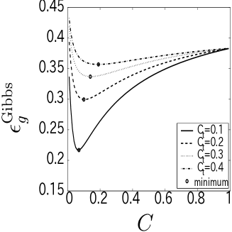
Two things are worth discussing further. Firstly, the simplest replica symmetry was assumed in the above analysis, the validity of which should be examined. In fact, the RS ansatz can be broken for sufficiently small $C$, for which certain replica symmetry breaking (RSB) analysis [9] is required. However, at the optimal choice of hyper parameter $C=C_{\rm t}$, the analysis can be considered to be correct because this choice of prior corresponds to the Nishimori condition known in spin-glass research at which no RSB is expected to occur [10]. Therefore, we do not perform RSB analysis in this paper. Secondly, the above analysis implies that minimization of the generalization error can be used to estimate hyper parameters for the SBC, which will be employed for a real world problem in a later section. However, this is not necessarily the case for other learning strategies. For example, Gibbs learning, which was extensively examined in the last few decades [7, 11] may be used for the classification. In this, the classification label for novel data is $\hat{y}^{\rm Gibbs}=\mathop{\rm argmax}_{y=\pm 1}\left\{f\left(\frac{y}{\sqrt{N}}\sum_{l=1}^{N}c_{l}w_{l}x_{l}\right)\right\}$, using a pair of parameters $\bm{w}$ and $\bm{c}$ that are randomly selected from the posterior distribution of eq. (5). The generalization error of this approach can be assessed as

$$\epsilon_{g}^{\rm Gibbs}=2\int Dz\left(1-\int Dvf\left(\sqrt{C_{\rm t}-\frac{R^{2}}{Q}}v+\frac{R}{\sqrt{Q}}z\right)\right)\int Du\Theta\left(f\left(\sqrt{C-Q}u+\sqrt{Q}z\right)-\frac{1}{2}\right),$$ (18)

using $R$ and $Q$. Although such a strategy may seem somewhat similar to using the SBC, the generalization error of this is not minimized at $C=C_{\rm t}$, as shown in fig. 1 (b), which indicates that minimizing $\epsilon_{g}^{\rm Gibbs}$ is not useful for identifying $C$. This may be a reason why the determination of hyper parameters was not discussed in preceding work of ref. [4], in which only variants of Gibbs learning were examined.

4 Development of a BP-Based Tractable Algorithm

The analysis in the preceding section indicates that the SBC of eq. (6) can provide optimal performance for a relation that is typically generated from eq. (7). Unfortunately, exact performance of the SBC is computationally difficult because a high-dimensional integration or summation with respect to $\bm{w}$ and $\bm{c}$ is required. Regarding this difficulty, recent studies [12, 13, 14] have shown that an algorithm termed belief propagation (BP), which was developed in the information sciences [15, 16], can serve as an excellent approximation algorithm. Therefore, let us try to construct a practically tractable algorithm for the SBC based on BP.

4.1 Belief Propagation

For this, we first pictorially represent the posterior distribution of eq. (5) by a complete bipartite graph, shown in fig. 2. In this figure, two types of nodes stand for the pairs of parameters $(w_{l},c_{l})$ (circle) and labels $y^{\mu}$ (square), while the edges connecting these nodes denote the components of the data $x_{l}^{\mu}$. We approximate the microcanonical prior of eq. (4) by a factorizable canonical prior as

$$P(\bm{w},\bm{c})\propto\prod_{l=1}^{N}\exp\left(-\frac{1}{2}(1-c_{l}+Gc_{l})w_{l}^{2}+\lambda c_{l}\right),$$ (19)

where $G>0$ and $\lambda$ are adjustable hyper parameters. Then, BP is defined as an algorithm that updates the two types of function of $(w_{l},c_{l})$, which are termed messages, as

$$\hat{{\mathcal{M}}}_{\mu\to l}^{t+1}(w_{l},c_{l}) =\frac{\int\prod_{j\neq l}dw_{j}\sum_{\bm{c}\backslash c_{l}}f\left(\Delta_{\mu}\right)\prod_{j\neq l}{\mathcal{M}}_{j\to\mu}^{t}(w_{j},c_{j})}{\int d\bm{w}\sum_{\bm{c}}f\left(\Delta_{\mu}\right)\prod_{j\neq l}{\mathcal{M}}_{j\to\mu}^{t}(w_{j},c_{j})},$$ (20)

$${\mathcal{M}}_{l\to\mu}^{t}(w_{l},c_{l}) =\frac{e^{-\frac{1}{2}(1-c_{l}+Gc_{l})w_{l}^{2}+\lambda c_{l}}\prod_{\nu\neq\mu}\hat{{\mathcal{M}}}_{\nu\to l}^{t}(w_{l},c_{l})}{\int dw_{l}\sum_{c_{l}}e^{-\frac{1}{2}(1-c_{l}+Gc_{l})w_{l}^{2}+\lambda c_{l}}\prod_{\nu\neq\mu}\hat{{\mathcal{M}}}_{\nu\to l}^{t}(w_{l},c_{l})},$$ (21)

between the two types of nodes, where $\Delta_{\mu}=\frac{y^{\mu}}{\sqrt{N}}\sum_{l=1}^{N}c_{l}w_{l}x_{l}^{\mu}$ and $t$ denotes the number of updates. ${\mathcal{M}}^{t}_{l\to\mu}(w_{l},c_{l})$ and $\hat{{\mathcal{M}}}_{\mu\to l}^{t}(w_{l},c_{l})$ are approximations at the $t$-th update of the marginal probability of a cavity system in which a single element of data $(\bm{x}^{\mu},y^{\mu})$ is left out from $D^{M}$ and the effective influence on $(w_{l},c_{l})$ when $\bm{x}^{\mu}$ is newly introduced to the cavity system, respectively. These provide an approximation of the posterior marginal at each update, which is termed the belief, given by

$$P(w_{l},c_{l}|D^{M})=\int\prod_{j\neq l}dw_{j}\sum_{\bm{c}\backslash c_{l}}P(\bm{w},\bm{c}|D^{M})\simeq\frac{e^{-\frac{1}{2}(1-c_{l}+G^{t}c_{l})w_{l}^{2}+\lambda^{t}c_{l}}\prod_{\mu=1}^{M}\hat{{\mathcal{M}}}_{\mu\to l}^{t}(w_{l},c_{l})}{\int dw_{l}\sum_{c_{l}}e^{-\frac{1}{2}(1-c_{l}+G^{t}c_{l})w_{l}^{2}+\lambda^{t}c_{l}}\prod_{\mu=1}^{M}\hat{{\mathcal{M}}}_{\mu\to l}^{t}(w_{l},c_{l})}.$$ (22)

At each update, the hyper parameters $G^{t}$ and $\lambda^{t}$ are determined so that the pruning constraints $\sum_{l=1}^{N}c_{l}=NC$ and $\sum_{l=1}^{N}c_{l}w_{l}^{2}=NC$ are satisfied on average with respect to eq. (22), which is valid for large $N$ due to the law of large numbers.

Figure 2: Complete bipartite graph representing the posterior distribution of eq. (5).

4.2 Gaussian Approximation and Self-Averaging Properties

Exactly evaluating eq. (20) is, unfortunately, still difficult. In order to resolve this difficulty, we introduce the Gaussian approximation:

$$\Delta_{\mu}\simeq\frac{y^{\mu}x_{l}^{\mu}}{\sqrt{N}}c_{l}w_{l}+\frac{1}{\sqrt{N}}\sum_{j\neq l}{y^{\mu}x_{j}^{\mu}}m_{j\to\mu}^{t}+\sqrt{V_{\mu\backslash l}^{t}}u,$$ (23)

where $u\sim{\cal N}(0,1)$, $m_{j\to\mu}^{t}=\int dw_{j}\sum_{c_{j}}(c_{j}w_{j}){\mathcal{M}}^{t}_{j\to\mu}(w_{j},c_{j})$ and $V_{\mu\backslash l}^{t}$ represents the variance of $\Delta_{\mu\backslash l}=\frac{1}{\sqrt{N}}\sum_{j\neq l}y^{\mu}x_{j}^{\mu}c_{l}w_{l}$. This approximation is likely to typically hold for large $N$ due to the central limit theorem when the parameters $(w_{j\neq l},c_{j\neq l})$ are generated from the cavity distribution $\prod_{j\neq l}{\mathcal{M}}_{j\to\mu}^{t}(w_{j},c_{j})$ in the case when the training data $\bm{x}^{\mu}$ are independently generated from $P_{\rm sph}(\bm{x})$. Further, we assume that the self-averaging property holds for $V_{\mu\backslash l}^{t}$, which implies that $V_{\mu\backslash l}^{t}$ typically converges to its sample average independently of $\bm{x}^{\mu}$ and can be evaluated using the $t$-th belief of eq. (22) as

$$V_{\mu\backslash l}^{t} =\left\langle\left(\Delta_{\mu\backslash l}-\left\langle\Delta_{\mu\backslash l}\right\rangle_{\mu}^{t}\right)^{2}\right\rangle_{\mu}^{t}=\frac{1}{N}\sum_{j,k\neq l}x_{j}^{\mu}x_{k}^{\mu}\left\langle(c_{j}w_{j}-m_{j\to\mu}^{t})(c_{k}w_{k}-m_{k\to\mu}^{t})\right\rangle_{\mu}^{t}$$ (24)

$$\to\frac{1}{N}\sum_{j,k\neq l}\overline{x_{j}^{\mu}x_{k}^{\mu}}\left\langle(c_{j}w_{j}-m_{j\to\mu}^{t})(c_{k}w_{k}-m_{k\to\mu}^{t})\right\rangle_{\mu}^{t}=\frac{1}{N}\sum_{j,k\neq l}\delta_{jk}\left\langle(c_{j}w_{j}-m_{j\to\mu}^{t})(c_{k}w_{k}-m_{k\to\mu}^{t})\right\rangle_{\mu}^{t}$$ (25)

$$=\frac{1}{N}\sum_{j\neq l}\left(\left\langle(c_{j}w_{j})^{2}\right\rangle_{\mu}^{t}-(m_{j\to\mu}^{t})^{2}\right)\simeq\frac{1}{N}\sum_{l=1}^{N}\left(\left\langle(c_{l}w_{l})^{2}\right\rangle^{t}-(m_{l}^{t})^{2}\right)=C-Q^{t},$$ (26)

where $\left\langle\cdots\right\rangle_{\mu}^{t}$ and $\left\langle\cdots\right\rangle^{t}$ denote averages over the cavity distribution $\prod_{j\neq l}{\mathcal{M}}_{j\to\mu}^{t}(w_{j},c_{j})$ and the belief of eq. (22), respectively, $m_{l}^{t}=\left\langle c_{l}w_{l}\right\rangle^{t}$ and $Q^{t}=\frac{1}{N}\sum_{l=1}^{N}(m_{l}^{t})^{2}$. We note that this property was once assumed to hold in equilibrium for similar systems [17, 18]. We here further assume that this can be extended even to the transient stage in BP dynamics [13, 14]. This provides an expression of eq. (20):

$$\hat{{\mathcal{M}}}_{\mu\to l}^{t+1}(w_{l},c_{l})\propto\exp\left[\frac{y^{\mu}x_{l}^{\mu}}{\sqrt{N}}a_{\mu\to l}^{t+1}(c_{l}w_{l})+\frac{(y^{\mu}x_{l}^{\mu})^{2}}{2N}b_{\mu\to l}^{t+1}(c_{l}w_{l})^{2}+O(N^{-3/2})\right],$$ (27)

where

$$a_{\mu\to l}^{t+1}=\frac{\partial\ln\left[\int Duf\left(\sqrt{C-Q^{t}}u+\left\langle\Delta_{\mu\backslash l}\right\rangle_{\mu}^{t}\right)\right]}{\partial\left\langle\Delta_{\mu\backslash l}\right\rangle_{\mu}^{t}}=\frac{\int Duf^{\prime}\left(\sqrt{C-Q^{t}}u+\left\langle\Delta_{\mu\backslash l}\right\rangle_{\mu}^{t}\right)}{\int Duf\left(\sqrt{C-Q^{t}}u+\left\langle\Delta_{\mu\backslash l}\right\rangle_{\mu}^{t}\right)},$$ (28)

$$b_{\mu\to l}^{t+1} =\left(\frac{\partial}{\partial\left\langle\Delta_{\mu\backslash l}\right\rangle_{\mu}^{t}}\right)^{2}\ln\left[\int Duf\left(\sqrt{C-Q^{t}}u+\left\langle\Delta_{\mu\backslash l}\right\rangle_{\mu}^{t}\right)\right]$$

$$=\frac{\int Duf^{\prime\prime}\left(\sqrt{C-Q^{t}}u+\left\langle\Delta_{\mu\backslash l}\right\rangle_{\mu}^{t}\right)}{\int Duf\left(\sqrt{C-Q^{t}}u+\left\langle\Delta_{\mu\backslash l}\right\rangle_{\mu}^{t}\right)}-(a_{\mu\to l}^{t+1})^{2},$$ (29)

Inserting these into eq. (21) offers the cavity average $m_{l\to\mu}^{t}$ as

$$m_{l\to\mu}^{t}=\frac{\frac{1}{\sqrt{F^{t}+\hat{Q}^{t}}}\exp\left[\lambda^{t}+\frac{(h_{l\backslash\mu}^{t})^{2}}{2(F^{t}+\hat{Q}^{t})}\right]}{1+\frac{1}{\sqrt{F^{t}+\hat{Q}^{t}}}\exp\left[\lambda^{t}+\frac{(h_{l\backslash\mu}^{t})^{2}}{2(F^{t}+\hat{Q}^{t})}\right]}\frac{h_{l\backslash\mu}^{t}}{F^{t}+\hat{Q}^{t}},$$ (30)

where $h_{l\backslash\mu}^{t}=\frac{1}{\sqrt{N}}\sum_{\nu\neq\mu}y^{\nu}x_{l}^{\nu}a_{\nu\to l}^{t}$ and we have introduced the novel macroscopic parameters

$$F^{t} =G^{t}-\frac{1}{N}\sum_{\nu\neq\mu}^{N}\frac{\int Duf^{\prime\prime}\left(\sqrt{C-Q^{t-1}}u+\left\langle\Delta_{\nu\backslash l}\right\rangle_{\nu}^{t-1}\right)}{\int Duf\left(\sqrt{C-Q^{t-1}}u+\left\langle\Delta_{\nu\backslash l}\right\rangle_{\nu}^{t-1}\right)}$$

$$\simeq G^{t}-\frac{1}{N}\sum_{\mu=1}^{N}\frac{\int Duf^{\prime\prime}\left(\sqrt{C-Q^{t-1}}u+\left\langle\Delta_{\mu}\right\rangle_{\mu}^{t-1}\right)}{\int Duf\left(\sqrt{C-Q^{t-1}}u+\left\langle\Delta_{\mu}\right\rangle_{\mu}^{t-1}\right)},$$ (31)

$$\hat{Q}^{t} =\frac{1}{N}\sum_{\nu\neq\mu}(a_{\nu\to l}^{t})^{2}\simeq\frac{1}{N}\sum_{\mu=1}^{M}\left(\frac{\int Duf^{\prime}\left(\sqrt{C-Q^{t-1}}u+\left\langle\Delta_{\mu}\right\rangle_{\mu}^{t-1}\right)}{\int Duf\left(\sqrt{C-Q^{t-1}}u+\left\langle\Delta_{\mu}\right\rangle_{\mu}^{t-1}\right)}\right)^{2},$$ (32)

assuming the further self-averaging property

$$\sum_{\nu\neq\mu}\frac{(y^{\nu}x_{l}^{\nu})^{2}}{N}b_{\nu\to l}^{t}\to\sum_{\mu=1}^{M}\frac{\overline{(y^{\mu}x_{l}^{\mu})^{2}}}{N}b_{\mu\to l}^{t}\simeq\frac{1}{N}\sum_{\mu=1}^{M}b_{\mu\to l}^{t}$$

$$\simeq\frac{1}{N}\sum_{\mu=1}^{M}\left(\frac{\partial}{\partial\left\langle\Delta_{\mu}\right\rangle_{\mu}^{t-1}}\right)^{2}\ln\left[\int Duf\left(\sqrt{C-Q^{t-1}}u+\left\langle\Delta_{\mu}\right\rangle_{\mu}^{t-1}\right)\right]\equiv\Gamma^{t}.$$ (33)

In eq. (30), the adjustable hyper parameters $F^{t}$ and $\lambda^{t}$ are determined so that the average pruning conditions

$$\frac{1}{N}\sum_{l=1}^{N}\langle c_{l}w_{l}^{2}\rangle^{t}=\frac{1}{N}\sum_{l=1}^{N}\dfrac{\frac{1}{\sqrt{F^{t}+\hat{Q}^{t}}}\exp\left[\lambda^{t}+\frac{(h_{l}^{t})^{2}}{2(F^{t}+\hat{Q}^{t})}\right]}{1+\frac{1}{\sqrt{F^{t}+\hat{Q}^{t}}}\exp\left[\lambda^{t}+\frac{(h_{l}^{t})^{2}}{2(F^{t}+\hat{Q}^{t})}\right]}\left(\frac{1}{F^{t}+\hat{Q}^{t}}+\frac{(h_{l}^{t})^{2}}{(F^{t}+\hat{Q}^{t})^{2}}\right)=C,$$ (34)

$$\frac{1}{N}\sum_{l=1}^{N}\langle c_{l}\rangle^{t}=\frac{1}{N}\sum_{l=1}^{N}\dfrac{\frac{1}{\sqrt{F^{t}+\hat{Q}^{t}}}\exp\left[\lambda^{t}+\frac{(h_{l}^{t})^{2}}{2(F^{t}+\hat{Q}^{t})}\right]}{1+\frac{1}{\sqrt{F^{t}+\hat{Q}^{t}}}\exp\left[\lambda^{t}+\frac{(h_{l}^{t})^{2}}{2(F^{t}+\hat{Q}^{t})}\right]}=C,$$ (35)

hold for eq. (22) at each update, where $h_{l}^{t}=\frac{1}{\sqrt{N}}\sum_{\mu=1}^{M}y^{\mu}x_{l}^{\mu}a_{\mu\to l}^{t}$.

Notice that eqs. (28)-(35) can be used as a computationally tractable algorithm for assessing the SBC. For this, we evaluate the posterior average $m_{l}=\left\langle c_{l}w_{l}\right\rangle$, plugging eq. (27) into eq. (22) using eqs. (28) and (29), which provides

$$m_{l}^{t}=\dfrac{\frac{1}{\sqrt{F^{t}+\hat{Q}^{t}}}\exp\left[\lambda^{t}+\frac{(h_{l}^{t})^{2}}{2(F^{t}+\hat{Q}^{t})}\right]}{1+\frac{1}{\sqrt{F^{t}+\hat{Q}^{t}}}\exp\left[\lambda^{t}+\frac{(h_{l}^{t})^{2}}{2(F^{t}+\hat{Q}^{t})}\right]}\frac{h_{l}^{t}}{F^{t}+\hat{Q}^{t}}.$$ (36)

This makes it possible to evaluate the SBC of eq. (6) using the Gaussian approximation as

$$\hat{y}={\rm sign}\left(Duf(\sqrt{C-Q^{t}}u+\left\langle\Delta\right\rangle^{t})-\frac{1}{2}\right),$$ (37)

for an element of data $\bm{x}$ that is newly generated from $P_{\rm sph}(\bm{x})$ at each update.

4.3 Further Reduction of Computational Cost

The necessary cost of performing the above procedure is $O(N^{2}M)$ per update, which can be further reduced. In order to save the computational cost, we represent $\left\langle\Delta_{\mu\backslash l}\right\rangle_{\mu}^{t}$ and $h_{l\backslash\mu}^{t}$ as

$$\left\langle\Delta_{\mu\backslash l}\right\rangle_{\mu}^{t} \simeq\left\langle\Delta_{\mu}\right\rangle^{t}-\frac{1}{\sqrt{N}}\sum_{l=1}^{N}y^{\mu}x_{l}^{\mu}\frac{\partial m_{l}^{t}}{\partial h_{l}^{t}}\left(\frac{y^{\mu}x_{l}^{\mu}}{\sqrt{N}}a_{\mu\to l}^{t}\right)-\frac{y^{\mu}x_{l}^{\mu}}{\sqrt{N}}m_{l\to\mu}^{t}\simeq\left\langle\Delta_{\mu}\right\rangle^{t}-\Xi^{t}a_{\mu}^{t}-\frac{y^{\mu}x_{l}^{\mu}}{\sqrt{N}}m_{l}^{t},$$ (38)

$$h_{l\backslash\mu}^{t} \simeq\theta_{l}^{t}-\frac{1}{\sqrt{N}}\sum_{\mu=1}^{M}y^{\mu}x_{l}^{\mu}\frac{\partial a_{\mu}^{t}}{\partial\left\langle\Delta_{\mu}\right\rangle_{\mu}^{t}}\left(\frac{y^{\mu}x_{l}^{\mu}}{\sqrt{N}}m_{l\to\mu}^{t-1}\right)-\frac{y^{\mu}x_{l}^{\mu}}{\sqrt{N}}a_{\mu\to l}^{t}\simeq\theta_{l}^{t}-\Gamma^{t}m_{l}^{t-1}-\frac{y^{\mu}x_{l}^{\mu}}{\sqrt{N}}a_{\mu}^{t},$$ (39)

using the singly-indexed variables $m_{l}^{t}$, $a_{\mu}^{t}=\frac{\partial\ln\left[\int Duf(\sqrt{C-Q^{t-1}}+\left\langle\Delta_{\mu}\right\rangle^{t-1}_{\mu})\right]}{\partial\left\langle\Delta_{\mu}\right\rangle^{t-1}_{\mu}}$, and $\left\langle\Delta_{\mu}\right\rangle^{t}=\frac{1}{\sqrt{N}}\sum_{l=1}^{N}y^{\mu}x_{l}^{\mu}m_{l}^{t}$, where $\theta_{l}^{t}=\frac{1}{\sqrt{N}}\sum_{\mu=1}^{M}y^{\mu}x_{l}^{\mu}a_{\mu}^{t}$ and $\Xi^{t}\equiv C-Q^{t}$. Using these, the algorithm developed above can be summarized as

$$a_{\mu}^{t+1} =\frac{\partial\ln\left[\int Duf\left(\sqrt{C-Q^{t}}u+\left\langle\Delta_{\mu}\right\rangle^{t}-\Xi^{t}a_{\mu}^{t}\right)\right]}{\partial\left\langle\Delta_{\mu}\right\rangle^{t}},$$ (40)

$$m_{l}^{t} =\frac{\partial\ln\left[1+\frac{1}{\sqrt{F^{t}+\hat{Q}^{t}}}\exp\left[\lambda^{t}+\frac{\left(\theta_{l}^{t}-\Gamma^{t}m_{l}^{t-1}\right)^{2}}{2(F^{t}+\hat{Q}^{t})}\right]\right]}{\partial\theta_{l}^{t}}.$$ (41)

This version may be useful in analyzing relatively higher dimensional data, as the computational cost per update is reduced from $O(N^{2}M)$ to $O(NM)$.

4.4 Performance Analysis and Link to the RS Solution

To investigate the performance of the BP-based algorithm, let us describe its behavior using macroscopic variables, such as $Q^{t}=\frac{1}{N}\sum_{l=1}^{N}(m_{l}^{t})^{2}$ and $R^{t}=\frac{1}{N}\sum_{l=1}^{N}w_{ol}m_{l}^{t}$, in the thermodynamic limit $N,M\to\infty$, keeping $\alpha\sim O(1)$. We will perform the analysis based on the naive expression of the algorithm in eqs. (28)-(35), since eqs. (40) and (41) are just a cost-saving version of this naive algorithm and, therefore, their behavior is identical.

For this purpose, we first assume that the self-averaging properties

$$\frac{1}{N}\bm{m}_{\mu}^{t}\cdot\bm{m}_{\mu}^{t} \simeq\frac{1}{N}\bm{m}^{t}\cdot\bm{m}^{t}=Q^{t},$$ (42)

$$\frac{1}{N}\bm{w}_{o}\cdot\bm{m}_{\mu}^{t} \simeq\frac{1}{N}\bm{w}_{o}\cdot\bm{m}^{t}=R^{t},$$ (43)

hold for the macroscopic variables. That the training data $\bm{x}^{\mu}$ are independently drawn from $P_{\rm sph}(\bm{x})$, in conjunction with the central limit theorem, implies that the pair of $\left\langle\Delta_{\mu}\right\rangle_{\mu}^{t}$ and the teacher’s stability $\Delta_{\mu}^{o}=\frac{y^{\mu}}{\sqrt{N}}\sum_{l=1}^{N}x_{l}^{\mu}w_{ol}$ can be treated as zero-mean Gaussian random variables, the variances and covariance of which are

$$\left[(\Delta^{o}_{\mu})^{2}\right]_{D^{M}}=\frac{\bm{w}_{o}\cdot\bm{w}_{o}}{N}\simeq C_{\rm t},\quad\left[\Delta^{o}_{\mu}\left\langle\Delta_{\mu}\right\rangle_{\mu}^{t}\right]_{D^{M}}\simeq R^{t},\quad\left[\left(\left\langle\Delta_{\mu}\right\rangle_{\mu}^{t}\right)^{2}\right]_{D^{M}}\simeq Q^{t}.$$ (44)

This makes it possible to represent these variables as

$$\Delta^{o}_{\mu}\simeq\sqrt{C_{\rm t}-\frac{(R^{t})^{2}}{Q^{t}}}v+\frac{R^{t}}{\sqrt{Q^{t}}}z,$$ (45)

$$\left\langle\Delta_{\mu}\right\rangle_{\mu}^{t}\simeq\sqrt{C-Q^{t}}u+\sqrt{Q^{t}}z,$$ (46)

using three independent Gaussian random variables $u,v,z\sim{\cal N}(0,1)$, which, in conjunction with the self-averaging property, indicates that the macroscopic properties of the cavity field $h_{l\backslash\mu}^{t+1}=\frac{1}{\sqrt{N}}\sum_{\nu\neq\mu}{y^{\nu}}x_{l}^{\nu}a_{\nu\to l}^{t+1}$ can be characterized independently of $l$ and $\mu$ as

$$\frac{1}{N}\sum_{l=1}^{N}(h_{l\backslash\mu}^{t+1})^{2}=\frac{1}{N^{2}}\sum_{l=1}^{N}\sum_{\mu,\nu}\left[y^{\mu}y^{\nu}x_{l}^{\mu}x_{l}^{\nu}a_{\mu\to l}^{t+1}a_{\nu\to l}^{t+1}\right]_{D^{M}}$$

$$\simeq\frac{1}{N^{2}}\sum_{l=1}^{N}\sum_{\mu=1}^{M}\left[(a^{t+1}_{\mu\to l})^{2}\right]_{D^{M}}\simeq\frac{1}{N^{2}}\sum_{l=1}^{N}\sum_{\mu=1}^{M}\left[(a^{t+1}_{\mu})^{2}\right]_{D^{M}}$$

$$\simeq 2\alpha\int DzDvf\left(\sqrt{C_{\rm t}-\frac{(R^{t})^{2}}{Q^{t}}}v+\frac{R^{t}}{\sqrt{Q^{t}}}z\right)\left(\frac{\int Duf^{\prime}\left(\sqrt{C-Q^{t}}u+\sqrt{Q^{t}}z\right)}{\int Duf\left(\sqrt{C-Q^{t}}u+\sqrt{Q^{t}}z\right)}\right)^{2}\simeq\hat{Q}^{t+1},$$ (47)

$$\frac{1}{N}\sum_{l=1}^{N}w_{ol}h_{l\backslash\mu}^{t+1}=\frac{1}{N}\sum_{l=1}^{N}\sum_{\nu\neq\mu}^{M}\left[\frac{y^{\nu}}{\sqrt{N}}x_{l}^{\nu}w_{ol}a_{\nu\to l}^{t+1}\right]_{D^{M}}$$

$$\simeq\frac{1}{N}\sum_{\mu=1}^{M}\left[\Delta_{\mu}^{o}a_{\mu}^{t+1}\right]_{D^{M}}-\frac{1}{N}\sum_{\mu=1}^{M}\sum_{l=1}^{N}w_{ol}m_{l\to\mu}^{t}\left[(y^{\mu}x_{l}^{\mu})^{2}\frac{\partial a_{\mu}^{t+1}}{\partial\left\langle\Delta_{\mu}\right\rangle_{\mu}^{t}}\right]_{D^{M}}$$

$$\simeq 2\alpha\int DzDv\left(\sqrt{C_{\rm t}-\frac{(R^{t})^{2}}{Q^{t}}}v+\frac{R^{t}}{\sqrt{Q^{t}}}z\right)f\left(\sqrt{C_{\rm t}-\frac{(R^{t})^{2}}{Q^{t}}}v+\frac{R^{t}}{\sqrt{Q^{t}}}z\right)\frac{\int Duf^{\prime}\left(\sqrt{C-Q^{t}}u+\sqrt{Q^{t}}z\right)}{\int Duf\left(\sqrt{C-Q^{t}}u+\sqrt{Q^{t}}z\right)}$$

$$-2\alpha R^{t}\int DzDvf\left(\sqrt{C_{\rm t}-\frac{(R^{t})^{2}}{Q^{t}}}v+\frac{R^{t}}{\sqrt{Q^{t}}}z\right)\frac{\partial}{\partial(\sqrt{Q^{t}}z)}\left(\frac{\int Duf^{\prime}\left(\sqrt{C-Q^{t}}u+\sqrt{Q^{t}}z\right)}{\int Duf\left(\sqrt{C-Q^{t}}u+\sqrt{Q^{t}}z\right)}\right)$$

$$=2\alpha C_{\rm t}\int DzDvf^{\prime}\left(\sqrt{C_{\rm t}-\frac{(R^{t})^{2}}{Q^{t}}}v+\frac{R^{t}}{\sqrt{Q^{t}}}z\right)\frac{\int Duf^{\prime}\left(\sqrt{C-Q^{t}}u+\sqrt{Q^{t}}z\right)}{\int Duf\left(\sqrt{C-Q^{t}}u+\sqrt{Q^{t}}z\right)}=C_{\rm t}\hat{R}^{t+1},$$ (48)

where the prefactor $2$ in eqs. (47) and (48) has its root in the two possibilities of the label $y=\pm 1$. On the other hand, these equations mean that the cavity fields, which can also be treated as Gaussian random variables since $x_{l}^{\mu}$ are zero-mean and almost uncorrelated random variables, can be represented as

$$h_{l\backslash\mu}^{t}=\sqrt{\hat{Q}^{t}}z+\hat{R}^{t}w_{ol},$$ (49)

where $z\sim{\cal N}(0,1)$, which yields

$$Q^{t} \simeq\frac{1}{N}\sum_{l=1}^{N}(m_{l\to\mu}^{t})^{2}=\frac{1}{N}\sum_{l=1}^{N}\left(\frac{\frac{1}{\sqrt{F^{t}+\hat{Q}^{t}}}\exp\left[\lambda^{t}+\frac{(h_{l\backslash\mu}^{t})^{2}}{2(F^{t}+\hat{Q}^{t})}\right]}{1+\frac{1}{\sqrt{F^{t}+\hat{Q}^{t}}}\exp\left[\lambda^{t}+\frac{(h_{l\backslash\mu}^{t})^{2}}{2(F+\hat{Q}^{t})}\right]}\frac{h_{l\backslash\mu}^{t}}{F+\hat{Q}^{t}}\right)^{2}$$ (50)

$$=\int Dz\left\langle\left(\frac{\frac{1}{\sqrt{F^{t}+\hat{Q}^{t}}}\exp\left[\lambda^{t}+\frac{(\sqrt{\hat{Q}^{t}}z+\hat{R}^{t}w_{o})^{2}}{2(F^{t}+\hat{Q}^{t})}\right]}{1+\frac{1}{\sqrt{F^{t}+\hat{Q}^{t}}}\exp\left[\lambda^{t}+\frac{(\sqrt{\hat{Q}^{t}}z+\hat{R}^{t}w_{o})^{2}}{2(F^{t}+\hat{Q}^{t})}\right]}\frac{\sqrt{\hat{Q}^{t}}z+\hat{R}^{t}w_{o}}{F^{t}+\hat{Q}^{t}}\right)^{2}\right\rangle_{w_{o}},$$ (51)

$$R^{t} \simeq\frac{1}{N}\sum_{l=1}^{N}w_{ol}m_{l\to\mu}^{t}\simeq\frac{1}{N}\sum_{l=1}^{N}\frac{\frac{1}{\sqrt{F^{t}+\hat{Q}^{t}}}\exp\left[\lambda^{t}+\frac{(h_{l\backslash\mu}^{t})^{2}}{2(F^{t}+\hat{Q}^{t})}\right]}{1+\frac{1}{\sqrt{F^{t}+\hat{Q}^{t}}}\exp\left[\lambda^{t}+\frac{(h_{l\backslash\mu}^{t})^{2}}{2(F^{t}+\hat{Q}^{t})}\right]}\frac{w_{ol}h_{l\backslash\mu}^{t}}{F^{t}+\hat{Q}^{t}}$$ (52)

$$=\frac{\hat{R}^{t}}{F^{t}+\hat{Q}^{t}}\int Dz\left\langle\frac{\frac{1}{\sqrt{F^{t}+\hat{Q}^{t}}}\exp\left[\lambda^{t}+\frac{(\sqrt{\hat{Q}^{t}}z+\hat{R}^{t}w_{o})^{2}}{2(F^{t}+\hat{Q}^{t})}\right]}{1+\frac{1}{\sqrt{F^{t}+\hat{Q}^{t}}}\exp\left[\lambda^{t}+\frac{(\sqrt{\hat{Q}^{t}}z+\hat{R}^{t}w_{o})^{2}}{2(F^{t}+\hat{Q}^{t})}\right]}w_{o}^{2}\right\rangle_{w_{o}},$$ (53)

where $F^{t}$ and $\lambda^{t}$ are determined so that the pruning conditions

$$\int Dz\left\langle\frac{\frac{1}{\sqrt{F^{t}+\hat{Q}^{t}}}\exp\left[\lambda^{t}+\frac{(\sqrt{\hat{Q}^{t}}z+\hat{R}^{t}w_{o})^{2}}{2(F^{t}+\hat{Q}^{t})}\right]}{1+\frac{1}{\sqrt{F^{t}+\hat{Q}^{t}}}\exp\left[\lambda^{t}+\frac{(\sqrt{\hat{Q}^{t}}z+\hat{R}^{t}w_{o})^{2}}{2(F^{t}+\hat{Q}^{t})}\right]}\left(\frac{1}{F^{t}+\hat{Q}^{t}}+\left(\frac{\sqrt{\hat{Q}^{t}}z+\hat{R}^{t}w_{o}}{F^{t}+\hat{Q}^{t}}\right)^{2}\right)\right\rangle_{w_{o}}=C,$$ (54)

$$\int Dz\left\langle\frac{\frac{1}{\sqrt{F^{t}+\hat{Q}^{t}}}\exp\left[\lambda^{t}+\frac{(\sqrt{\hat{Q}^{t}}z+\hat{R}^{t}w_{o})^{2}}{2(F^{t}+\hat{Q}^{t})}\right]}{1+\frac{1}{\sqrt{F^{t}+\hat{Q}^{t}}}\exp\left[\lambda^{t}+\frac{(\sqrt{\hat{Q}^{t}}z+\hat{R}^{t}w_{o})^{2}}{2(F^{t}+\hat{Q}^{t})}\right]}\right\rangle_{w_{o}}=C,$$ (55)

hold for the $t$-th update.

Figure 3: Generalization error of SBC provided by the BP-based algorithm (40) and (41) after $t$th update. Markers were obtained from $100$ experiments for a transfer function $f(u;\kappa=0.05)=0.05+0.9\Theta(u)$ in the case of $C_{\rm t}=0.2$ varying $C=0.1,0.2$ and $0.3$. Error bars indicate 95% confidence intervals. Lines represent the theoretical prediction assessed by eqs. (47)-(55), which exhibits excellent consistency with the experimental results.

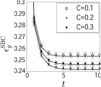
In fig. 3, experimentally obtained time evolution of the BP-based algorithm (40) and (41) is compared with its theoretical prediction assessed by eqs. (47)-(55), which exhibits excellent consistency. This validates the macroscopic analysis provided above. It is worth noting that the stationary conditions of eqs. (47)-(55) are identical to those of the saddle point of the RS free energy of eq. (16). This implies that the BP-based algorithm provides a nearly optimal solution in a practical time scale in assumed ideal situations of large system size if the hyper parameter $C_{\rm t}$ is correctly estimated.

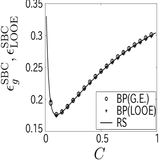
The replica analysis in the previous section indicates that $C_{\rm t}$ can be estimated by minimizing the generalization error $\epsilon_{g}^{\rm SBC}$. The leave-one-out error (LOOE), which is represented as

$$\epsilon_{\rm LOOE}^{\rm SBC}=\frac{1}{M}\sum_{\mu=1}^{M}\Theta\left(\frac{1}{2}-\int Duf\left(\sqrt{C-Q}u+\left\langle\Delta_{\mu}\right\rangle_{\mu}\right)\right),$$ (56)

in the current case, is frequently used as an estimate of $\epsilon_{g}^{\rm SBC}$ for practical applications, since it can be evaluated from only the training set $D^{M}$. The algorithm is also useful for assessing the LOOE of eq. (56), since this computes all the cavity stabilities $\left\langle\Delta_{\mu}\right\rangle_{\mu}$ at each update, which saves the cost of relearning in assessing the LOOE [18]. Fig. 4 shows a comparison between $\epsilon_{g}^{\rm SBC}$ and $\epsilon_{\rm LOOE}^{\rm SBC}$ for an activation function, as given in eq. (17), in the case of $N,M=2000$. It shows that the LOOE (56) can be used in practical applications for determining the necessary hyper parameters using only given data.

The BP-based algorithm of eqs. (40) and (41) is developed and analyzed under the self-averaging assumption, which is valid when each data $\bm{x}^{\mu}$ is independently sampled from the spherical distribution $P_{\textrm{sph}}(\bm{x})$. Unfortunately, raw real world data do not necessarily obey such distributions, which may deteriorate the approximation accuracy of the developed algorithm. A simple approach to handle this problem is to make statistical properties of the data set get closer to those of samples from $P_{\textrm{sph}}(\bm{x})$ by linearly transforming $\bm{x}^{\mu}$ so that $\frac{1}{M}\sum_{\mu=1}^{M}\mbox{\boldmath{$x$}}^{\mu}=0$ and $\frac{1}{M}\sum_{\mu=1}^{M}x_{i}^{\mu}x_{j}^{\mu}\simeq\delta_{ij}$ hold with keeping $|\bm{x}^{\mu}|$ fixed to the square root of the dimensionality. Such an approach is often termed whitening, the efficacy of which will be experimentally examined in the next section.

Figure 4: Comparison between $\epsilon_{g}^{\rm SBC}$ ($\circ$) and $\epsilon_{\rm LOOE}^{\rm SBC}$ ($+$) for $C_{\rm t}=0.1$,$\kappa=0.05$ and $\alpha=1$. $\epsilon_{g}^{\rm SBC}$ is evaluated by replica analysis under the replica symmetric ansatz (Line), while $\epsilon_{\rm LOOE}^{\rm SBC}$ is experimentally obtained using eqs. (40) and (41) for $N,M=2000$.

5 Application to a Real World Problem

To examine the practical significance of the SBC, we applied it to a real world problem. We considered the task of distinguishing cancer from normal tissue using microarray data of $N=2000$ dimensions [3]. The data was sampled from $M=62$ tissues, 20 and 42 tissues of which were classified as normal and cancerous, respectively.

We employed eq. (17) as the activation function. The data set $D^{M}=\{(\bm{x}^{\mu},y^{\mu})\}$ [19] was pre-processed so that $\frac{1}{M}\sum_{\mu=1}^{M}\bm{x}^{\mu}=0$ and $|\bm{x}^{\mu}|=\sqrt{N}$ held. The data set was randomly divided into training and test sets, which were composed of 42 and 20 tissues, respectively. For a given training set, the hyper parameters $C$ and $\kappa$ were determined from the possibilities of $C=\{2.5\times 10^{-3},5.0\times 10^{-3},1.0\times 10^{-2},5.0\times 10^{-2},0.1,0.2,0.4,0.6,0.8\}$ and $\kappa=\{0.1,0.2,0.3,0.4\}$, so as to minimize eq. (56) for the training set. After determining $C$ and $\kappa$, the generalization error was measured for the test set. We repeated this experiment 200 times, redividing the data set.

The results are shown in table 1. The conventional Fisher discriminant analysis (FDA) [20] and Sparse Bayesian learning (SBL) [21], which selects a sparse model using a certain prior, termed the automatic relevance determination (ARD) prior [22, 23], are presented for comparison. It is apparent that the FDA, which does not have a mechanism to reduce effective dimensions, exhibits a significantly lower generalization ability than the other two schemes. This is also supported by Welch’s test, which is a standard method to examine statistical significance of difference of averages between two groups, although the standard deviation of FDA is smaller than those of the others. On the other hand, although the average generalization error of the SBC is smaller than that of SBL, the standard deviations are large, which prevents us from clearly judging the superiority of the SBC.

In order to resolve this difficulty, we examined how many times the SBC provided a smaller generalization error than SBL in the 200 experiments. The number of times that the SBC offered smaller, equal and larger errors than SBL were 99, 36 and 65, respectively. A one-sided binomial test was applied to this result under the null hypothesis that there is no difference of the generalization ability between SBC and SBL ignoring the tie data, which yields $\frac{|99-(200-36)\times\frac{1}{2}|}{\sqrt{(200-36)\times\frac{1}{2}\times\frac{1}{2}}}=2.65\cdots>u(0.05)=1.64\cdots$ under the normal approximation. This implies that the difference between SBC and SBL is statistically significant with a confidence level of $95$% and, therefore, the SBC has a higher generalization ability.

Table 1: Classification result

	generalization error (%)	standard deviation
SBC	23.5	10.2
SBL	24.3	10.7
FDA	39.6	8.39

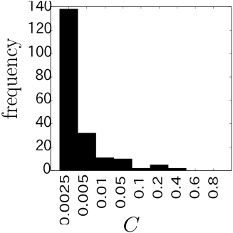
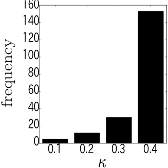
Histograms of selected values of $C$ and $\kappa$ are shown in figs. 5 and 6, respectively. They indicate that $\kappa$ has a statistically greater fluctuation. For reference, we performed experiments fixing $\kappa$ to the most frequent value, $\kappa=0.4$, which reduced the average and standard deviation of the generalization error of SBC to 21.0(%) and 9.72, respectively. This determination by the resampling technique is an alternative scheme for estimating hyper parameters. Although performing it naively requires a greater computational cost than minimizing the LOOE, a recently proposed analytical approximation method [24] may be promising for reducing computational cost, and will be the subject of future work.

In the algorithm we have developed, we assumed a self-averaging property. This assumption may give a good match with whitened data, i.e., data for which the dimensionality is reduced from $N=2000$ to $M=62$ by a linear transformation so that $\frac{1}{M}\sum_{\mu=1}^{M}\bm{x}^{\mu}=0$ and $\frac{1}{M}\sum_{\mu=1}^{M}x_{i}^{\mu}x_{j}^{\mu}=\delta_{ij}$ hold in the reduced space. We also carried out the above experiments for the whitened data fixing $\kappa$ to $0.4$, finding that the average and standard deviation of the generalization error of the SBC were reduced to 16.3(%) and 6.20, respectively. However, such an approach may not be preferred because it becomes difficult to interpret the implications of the result as the original meaning of variables is lost by the linear transformation.

Figure 5: Histogram of selected $C$

Figure 6: Histogram of selected $\kappa$

6 Summary

In summary, we have developed a classifier termed the sparse Bayesian classifier (SBC) that eliminates irrelevant components in high-dimensional data $\bm{x}\in\mathcal{R}^{N}$ by multiplying discrete variables $c_{l}\in\{0,1\},1\leq l\leq N$ for each dimension $l$ following the Bayesian framework. The efficacy of the SBC was confirmed by the replica method for the target rules of a certain type. Unfortunately, exactly evaluating the SBC is computationally difficult. In order to resolve this difficulty, we have also developed a computationally tractable approximation algorithm for the SBC based on belief propagation (BP). It turns out that the developed BP-based algorithm provides a result consistent with that of replica analysis for ideal situations, which implies that a nearly optimal performance can be obtained in a practical time scale in such ideal cases. Finally, the significance of the SBC to real world applications was experimentally validated for a problem of colon cancer classification.

In this paper, the classifier was developed for minimizing the generalization error. Identifying relevant components from a given data set may be another purpose of the classification analysis. Designing a classifier for this purpose is currently under way.

References

- [1] V. N. Vapnik, Statistical learning theory (John Wiley & Sons,New York, 1998).
- [2] Y. Iba, J. Phys. A 32, 3875 (1999).
- [3] Y. Li, C. Campbell, and M. Tipping, Bioinformatics 18, 1332 (2002).
- [4] P. Kuhlmann and K.-R. Müller, J. Phys. A 27, 3759 (1994).
- [5] Y. Iba, in Proceedings of ICONIP’98, edited by S. Usui and T. Omori (Ohmsha,Tokyo and IOS Press, Burke VA, 1998), vol. 1, pp. 530–533.
- [6] B. Scholkopf and S. J. Smola, Learning with kernels (The MIT Press, 2001).
- [7] T. H. Watkin, A. Rau, and M. Biehl, Rev. Mod. Phys. 65, 499 (1993).
- [8] H. Nishimori, Statistical Physics of Spin Glasses and Information Processing (Oxford University Press, 2001).
- [9] M. Mezard, G. Parisi, and M. A. Virasoro, Spin Glass Theory and Beyond (World Scientific(Singapore), 1987).
- [10] H. Nishimori, Prog. Theor. Phys. 66, 1169 (1981).
- [11] M. Opper, D. Haussler, Phys.Rev.Lett. 66, 2677 (1991).
- [12] D. J. C. MacKay, IEEE Trans. on Inf. Theor. 45, 399 (1999).
- [13] Y. Kabashima, J. Phys. Soc. Jpn 72, 1645 (2003a).
- [14] Y. Kabashima, J. Phys. A 36, 11111 (2003b).
- [15] R. G. Gallager, Low Density Parity Check Codes (The MIT Press, 1963).
- [16] J. Pearl, Probabilistic Reasoning in Intelligent Systems: Network of Plausible Inference (Morgan Kaufmann San Francisco, 1988).
- [17] M. Mezard, J. Phys. A 22, 2181 (1989).
- [18] M. Opper and O. Winther, in Advances in Neural Information Processing Systems, edited by M. C. Mozer, M. I. Jordan, and T. Petche (MIT press(Cambridge,MA), 1997), vol. 9, pp. 225–231.
- [19] U. Alon, N. Barkai, D. Notterman, K. Gish, S. Ybarra, D. Mack, and A. Levine, Cell Biol. 96, 6745 (1999).
- [20] R. A. Fisher, Annals of Eugenics 7, 179 (1936).
- [21] M. E. Tipping, Journal of Machine Learning Resarch 1, 211 (2001).
- [22] D. J. C. MacKay, in Models of Neural Networks III, edited by E. Domany, J. L. van Hemmen, and K. Schulten (Springer, 1994), chap. 6, pp. 211–254.
- [23] R. M. Neal, Baysian Learning for Neural Networks (Springer, New York, 1996).
- [24] D. Malzahn and M. Opper, Journal of Machine Learning Research 4, 1151 (2004).