We explore the role that random arbitrage opportunities play in hedging financial derivatives. We extend the asymptotic pricing theory presented by Fedotov and Panayides [Stochastic arbitrage return and its implication for option pricing, Physica A 345 (2005), 207-217] for the case of hedging a derivative when arbitrage opportunities are present in the market. We restrict ourselves to finding hedging confidence intervals that can be adapted to the amount of arbitrage risk an investor will permit to be exposed to. The resulting hedging bands are independent of the detailed statistical characteristics of the arbitrage opportunities.

PACS number: 02.50.Ey; 89.65.Gh

Keywords:

Derivative hedging, random arbitrage, hedging ratio.

1 Introduction

In the classical Black-Scholes methodology a perfect hedge is achieved by holding an amount $\frac{\partial V}{\partial S}$ of the underlying asset $S$ in order to eliminate the risk from the changes in the stock price [1]. When one of the Black-Scholes ideal assumptions is relaxed the procedure is less clear and alternative methods have to be proposed (see for example [2, 3, 4]). In this paper we relax the no-arbitrage assumption and study the hedging problem for the case arbitrage opportunities are stochastic.

Empirical studies have shown existence of short lived arbitrage opportunities [5, 6]. Thus, accepting that arbitrage opportunities do exist, one is forced to consider them when pricing and hedging a derivative. The first attempt to take into account arbitrage opportunities for pricing a derivative is given in [7, 8] where the constant interest rate $r_{0}$ is substituted by the stochastic process $r_{0}+x(t)$. The random arbitrage $x(t)$ is assumed to follow an Ornstein-Uhlenbeck process. In [9, 10] the same idea is reformulated in terms of option pricing with stochastic interest rate. For a more recent literature on arbitrage we refer the reader to [11, 12] and references therein.

In [13] Fedotov and Panayides present an asymptotic pricing theory, based on the central limit theorem [14], for pricing an option contract. The methodology focuses on deriving pricing bands for the option rather than finding an exact equation for the price. The nice feature of the method is that the pricing bands are independent of the detailed statistical characteristics of the random arbitrage. In this paper we apply the same methodology as for the pricing case and try to find hedging confidence intervals that can be adapted to the amount of arbitrage risk an investor will permit to be exposed to.

In section 2 we briefly review the methodology used in [13]. In section 3 we use the same technique to find hedging bands around the usual Black-Scholes hedging ratio that account for the arbitrage opportunities. Numerical calculations are presented in section 4. Concluding remarks are given in section 5.

2 Methodology

Following [13], consider a market that consists of a stock $S$, a bond $B$, and a European option on the stock $V$. The market is assumed to be affected by two sources of uncertainty, the random fluctuations of the return from the stock, and a random arbitrage return from the bond described respectively by the conventional stochastic differential equations

$$\frac{dS}{S}=\mu dt+\sigma dW,$$ (1)

and

$$\frac{dB}{B}=rdt+\xi(t)dt,$$ (2)

where $r$ is the risk-free interest rate, and $W$ the standard Wiener process. The random process $\xi(t)$ describes the fluctuations of the arbitrage return around $rdt$.

The random variations of arbitrage return $\xi(t)$ are assumed to be on the scale of hours. Denote this characteristic time by $\tau_{arb}$ and regard it as an intermediate one between the time scale of random stock return (infinitely fast Brownian motion fluctuations), and the lifetime of the derivative $T$ (several months): $0<<$ $\tau_{arb}<<T$. This difference in time allows the development of an asymptotic pricing theory involving the central limit theorem for random processes.

The next step is the derivation of the PDE satisfying the option price $V$. Consider the investor establishing a zero initial investment position by creating a portfolio $\Pi$ consisting of one bond $B,$ $-\frac{\partial V}{\partial S}$ shares of the stock $S$ and one European option $V$ with an exercise price $K$ and a maturity $T.$ The value of this portfolio is given by

$$\Pi=B-\frac{\partial V}{\partial S}S+V.$$ (3)

The Black-Scholes dynamic of this portfolio is given by the two equations $\partial\Pi/\partial t=0$ and $\ \Pi=0$ . The application of Itô’s formula to (3), together with (1) and (2) with $\xi(t)=0,$ leads to the classical Black-Scholes equation:

$$\frac{\partial V}{\partial t}+\frac{\sigma^{2}S^{2}}{2}\frac{\partial^{2}V}{\partial S^{2}}+rS\frac{\partial V}{\partial S}-rV=0.$$ (4)

A generalization of $\partial\Pi/\partial t=0$ is the simple non-equilibrium equation

$$\frac{\partial\Pi}{\partial t}=-\frac{\Pi}{\tau_{arb}},$$ (5)

where $\tau_{arb}$ is the characteristic time during which the arbitrage opportunity ceases to exist (see [15]). Using the self-financing condition $d\Pi=dB-\frac{\partial V}{\partial S}dS+dV$, Ito’s lemma, and equations (1) and (2), the equation for the option value $V(S,t)$ is easily shown to satisfy the PDE

$$\frac{\partial V}{\partial t}+\frac{\sigma^{2}S^{2}}{2}\frac{\partial^{2}V}{\partial S^{2}}+rS\frac{\partial V}{\partial S}-rV+r\Pi+\xi(t)\Pi+\xi(t)\left(S\frac{\partial V}{\partial S}-V\right)+\frac{\Pi}{\tau_{arb}}=0.$$ (6)

This equation reduces to the classical Black-Scholes PDE (4) when $\Pi=0$ and $\xi(t)=0.$

To deal with the forward problem lets introduce the non-dimensional time

$$\tau=\frac{T-t}{T},\;\;\;0\leq\tau\leq 1,$$ (7)

and a small parameter

$$\varepsilon=\frac{\tau_{arb}}{T}<<1.$$ (8)

In the limit $\varepsilon\rightarrow 0,$ the stochastic arbitrage return $\xi$ becomes a function that is rapidly varying in time, say $\xi\left(\frac{\tau}{\varepsilon}\right)$ (see [16]). The random arbitrage $\xi(\tau)$ is assumed to be an ergodic random process with  $<$ $\xi(\tau)$ $>=0,$ such that

$$D=\int_{0}^{\infty}<\xi(\tau+s)\xi(\tau)>ds$$ (9)

is finite. From (5) the value of the portfolio $\Pi$ decreases to zero exponentially. Thus, it is assumed that $\Pi$ $=0$ in the limit $\varepsilon\rightarrow 0$. From (6) the associated option price $V^{\varepsilon}=V^{\varepsilon}\left(\tau,S\right)$ obeys the stochastic PDE

$$\frac{\partial V^{\varepsilon}}{\partial\tau}=\frac{\sigma^{2}S^{2}}{2}\frac{\partial^{2}V^{\varepsilon}}{\partial S^{2}}+rS\frac{\partial V^{\varepsilon}}{\partial S}-rV^{\varepsilon}+\xi(\frac{\tau}{\varepsilon})\left(S\frac{\partial V^{\varepsilon}}{\partial S}-V^{\varepsilon}\right),$$ (10)

with the initial condition

$$V^{\varepsilon}(S,0)=\max(S-K,0)$$ (11)

for a call option with strike price $K$. Using the law of large numbers and the central limit theorem for stochastic processes (see [14]), Fedotov and Panayides analyze the stochastic PDE (10) and give pricing bands for the option. More details are given in [13].

3 Hedging Ratio

In this section we address the problem of hedging the risk from writing an option on an asset, for the case stochastic arbitrage opportunities are present in the market. Here, we apply the same methodology as for the pricing case used in [13], and try to find hedging confidence intervals that can be adapted to the amount of arbitrage risk an investor will permit to be exposed to. The method can be used to save on the cost of hedging in a random arbitrage environment.

In the usual Black-Scholes case a perfect hedge is achieved by holding an amount $\Delta_{BS}=\frac{\partial V}{\partial S}$ of the underlying asset in order to eliminate the risk from the changes in the stock price. Differentiating (4) with respect to $S$, and introducing the non-dimensional time $\tau$ as before, gives

$$\frac{\partial\Delta_{BS}}{\partial\tau}=S(\sigma^{2}+r)\frac{\partial\Delta_{BS}}{\partial S}+\frac{\sigma^{2}S^{2}}{2}\frac{\partial^{2}\Delta_{BS}}{\partial S^{2}},$$ (12)

with initial condition $\Delta_{BS}\left(S,0\right)=H(S-K)$ for a call option with strike price $K$ and $H$ the Heaviside function. Similarly, differentiating (10) with respect to $S$ the stochastic hedging ratio that accounts for the stochastic arbitrage returns, defined by $\Delta^{\varepsilon}=\frac{\partial V^{\varepsilon}}{\partial S}$ with $\varepsilon$ as before, satisfies the PDE

$$\frac{\partial\Delta^{\varepsilon}}{\partial\tau}=\sigma^{2}S\frac{\partial\Delta^{\varepsilon}}{\partial S}+\frac{\sigma^{2}S^{2}}{2}\frac{\partial^{2}\Delta^{\varepsilon}}{\partial S^{2}}+(r+\xi(\frac{\tau}{\varepsilon}))S\frac{\partial\Delta^{\varepsilon}}{\partial S}.$$ (13)

According to the law of large numbers, the stochastic hedging ratio $\Delta^{\varepsilon}=\Delta^{\varepsilon}\left(S,\tau\right)$ converges in probability to the Black-Scholes hedging ratio $\Delta_{BS}\left(S,\tau\right)$. Splitting $\Delta^{\varepsilon}=\frac{\partial V^{\varepsilon}}{\partial S},$ into the sum of the Black-Scholes hedging ratio $\Delta_{BS}\left(S,\tau\right),$ and the random field $Y^{\varepsilon}\left(S,\tau\right),$ with the scaling factor $\sqrt{\varepsilon}$, gives

$$\Delta^{\varepsilon}\left(S,\tau\right)=\Delta_{BS}\left(S,\tau\right)+\sqrt{\varepsilon}Y^{\varepsilon}\left(S,\tau\right).$$ (14)

Substituting (14) into (13), and using equation (12), we get the stochastic PDE for the random field $Y^{\varepsilon}\left(S,\tau\right)$, given by

$$\frac{\partial Y^{\varepsilon}}{\partial\tau}=\frac{1}{2}\sigma^{2}S^{2}\frac{\partial^{2}Y^{\varepsilon}}{\partial S^{2}}+(\sigma^{2}S+rS+\xi(\frac{\tau}{\varepsilon})S)\frac{\partial Y^{\varepsilon}}{\partial S}+\xi(\frac{\tau}{\varepsilon})\frac{S}{\sqrt{\varepsilon}}\frac{\partial\Delta_{BS}}{\partial S}.$$ (15)

In what follows, we try to find the asymptotic equation for $Y^{\varepsilon}\left(S,\tau\right)$ as $\varepsilon\rightarrow 0.$ Applying Ergodic theory, in the limit $\varepsilon\rightarrow 0,$ the random field $Y^{\varepsilon}\left(S,\tau\right)$ converges weakly to the field $Y\left(S,\tau\right)$ satisfying the linear stochastic PDE

$$\frac{\partial Y}{\partial\tau}=\frac{1}{2}\sigma^{2}S^{2}\frac{\partial^{2}Y}{\partial S^{2}}+S\left(\sigma^{2}+r\right)\frac{\partial Y}{\partial S}+S\frac{\partial\Delta_{BS}}{\partial S}\eta\left(\tau\right),$$ (16)

for $\eta\left(\tau\right)$ the white Gaussian noise satisfying

$$<\eta(\tau_{1})\eta(\tau_{2})>=2D\delta\left(\tau_{1}-\tau_{2}\right),$$ (17)

$D$ the diffusion constant given by (9), and with initial condition $Y\left(S,0\right)=0.$ The solution to equation (16) is given by

$$Y(\tau,S)=\int_{0}^{\tau}\int_{0}^{\infty}G(S,S_{1},\tau,\tau_{1})S_{1}\frac{\partial\Delta_{BS}}{\partial S_{1}}\eta\left(\tau_{1}\right)dS_{1}d\tau_{1},$$ (18)

where $G(S,S_{1},\tau,\tau_{1})$ is the Green’s function corresponding to (16) (see [17]). From the solution (18) it follows that  $Y(S,\tau)$ is a Gaussian field with zero mean and covariance $R(S,x,\tau)=<Y\left(S,\tau\right)Y(x,\tau)>$ satisfying the deterministic PDE

$$\frac{\partial R}{\partial\tau}=\frac{1}{2}\sigma^{2}S^{2}\frac{\partial^{2}R}{\partial S^{2}}+\frac{1}{2}\sigma^{2}x^{2}\frac{\partial^{2}R}{\partial x^{2}}+S\left(\sigma^{2}+r\right)\frac{\partial R}{\partial S}+x\left(\sigma^{2}+r\right)\frac{\partial R}{\partial x}+\\ 2D\left(S\frac{\partial\Delta_{BS}}{\partial S}\times x\frac{\partial\Delta_{BS}}{\partial x}\right),$$ (19)

with $R(S,x,0)\equiv 0$. The typical hedging bands for the case of arbitrage opportunities can be given by

$$\Delta_{BS}\left(S,\tau\right)\pm 2\sqrt{\varepsilon U\left(S,\tau\right)}.$$ (20)

Hedging within two standard deviations of the Black-Scholes hedging ratio provides a higher protection against arbitrage fluctuations. The variance $U\left(S,\tau\right)=R(S,S,\tau)$ quantifies the fluctuations around the Black-Scholes hedging ratio and is given by

$$U\left(S,\tau\right)=2D\int_{0}^{\tau}[\int_{0}^{\infty}G\left(S,S_{1},\tau,\tau_{1}\right)S_{1}\frac{\partial\Delta_{BS}}{\partial S_{1}}dS_{1}]^{2}d\tau_{1}.$$ (21)

One can conclude that the investor hedges the option using the hedging ratio

$$\Delta_{BS}\left(S,\tau\right)+2\sqrt{\varepsilon U\left(S,\tau\right)}.$$ (22)

4 Numerical Results

From equation (16) or (21) we can see that the large fluctuations of $Y(S,\tau)$ occur when the function $S\frac{\partial\Delta_{BS}}{\partial S}$ takes its maximum value. This is the case for near at-the money options. Thus, the risk error (bandwidth) in hedging an option is greater for these cases. Using equation (19) we get a plot of the covariance $U(S,\tau)$ with respect to asset price $S$ and time $\tau$ (Figure 1). From the graph we observe that the hedging error increase as we move near at-the-money. This result is consistent with the empirical results presented in [18, 19]. In Figure 2, we plot the effective hedging ratio given by equation (22), for $\varepsilon=0.1$, and compare it with the usual Black-Scholes hedging ratio. Note that the largest deviations from the usual Black-Scholes hedging ratio are near at-the money, while they decrease as we move in and out-of-the-money. In particular, the arbitrage corrections for near at-the-money account for approximately 3.5% change in the Black-Scholes hedging ratio.

5 Conclusions

Using an asymptotic pricing theory, first introduced by Fedotov and Panayides [13], we explored the role that random arbitrage opportunities play in hedging derivatives. In particular, we managed to give hedging bands around the usual Black-Scholes hedging ratio that account for the stochastic nature of arbitrage opportunities. Numerical results showed that the largest deviations from the usual Black-Scholes hedging ratio are near at-the money. Note that the work in this paper is purely theoretical. Despite this the results are consistent with empirical work in the literature. In future work we plan to address parametric and non-parametric statistical tests on a large sample of observations of trades to explain quantitatively any market deviations from the Black-Scholes price and hedge ratio for the case of arbitrage returns.

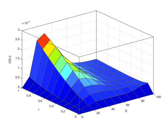
Figure 1: Variance $U(S,\tau)$, with respect to asset price $S$, and time $\tau$. The option strike price $K=20$, the volatility $\sigma=0.4$, the interest rate $r=0.1$, and the constant $D=0.1$.

Figure 2: Effective hedging ratio and Black-Scholes hedging ratio. Here $\varepsilon=0.1$, $T=1$ (years) and constants $K$, $\sigma$, $r$, and $D$ are taken as in Figure 1.

References

- [1] F. Black, M. Scholes, The pricing of options and corporate liabilities, J. Political Econ. 81 (1973) 637-659.
- [2] H. Follmer, D. Sondermann, Hedging of non-redundant contingent claims, In W. Hildenbrand and A. Mas-Colell (eds.), Contributions of Mathematical Economics (1986) 205-223.
- [3] M. Schweizer, Option hedging, Stoch. Process Appl. 37 (1991) 339-363.
- [4] E. Renault, N. Touzi, Option hedging and implied volatilities in a stochastic volatility model Mathematical Finance 6 (3) (1996) 279-302.
- [5] D. Galai, Tests of market efficiency and the Chicago board option exchange, J. Bus. 50 (1977) 167-197.
- [6] G. Sofianos, Index arbitrage profitability, NYSE working paper 90-04, J. Derivatives 1 (N1) (1993).
- [7] K. Ilinsky, How to account for the virtual arbitrage in the standard derivative pricing, preprint, cond-mat/9902047.
- [8] K. Ilinsky, A. Stepanenko, Derivative pricing with virtual arbitrage, preprint, cond-mat/9902046.
- [9] M. Otto, Stochastic relaxation dynamics applied to finance: towards non-equilibrium option pricing theory, Eur. Phys. J. B 14 (2000) 383-394.
- [10] M. Otto, Towards non-equilibrium option pricing theory, Int. J. Theor. Appl. Finance 3(3) (2000) 565.
- [11] M. Ammann, S. Herriger, Relative Implied-Volatility Arbitrage with Index Options Financial Analysts Journal 58(6) (2002).
- [12] K. Ilinski, Physics of Finance, Wiley & Sons, (2001).
- [13] S. Fedotov, S. Panayides, Stochastic arbitrage return and its implication for option pricing, Physica A 345 (2005) 207-217.
- [14] M. I. Freidlin, A. D. Wentzell, Random perturbations of dynamical systems, Springer, New York, 1984.
- [15] A. N. Adamchuk, S. E Esipov, Collectively fluctuating assets in the presence of arbitrage opportunities and option pricing, Phys. Usp. 40 (12) (1997) 1239-1248.
- [16] G. Papanicolaou, R. Sircar, Stochastic volatility, smiles and asymptotics, Appl. Math. Finance 6 (1999) 107-145.
- [17] R. Courant, D. Hilbert, Methods of Mathematical Physics, vol. II, Partial Differential Equations, Wiley, New York 1989.
- [18] G. Bakshi, C. Cao, Z. Chen, Empirical performance of alternative option pricing models, J. Finance (1997) 2003-2049.
- [19] G. Bakshi, C. Cao, Z. Chen, Pricing and Hedging Long-Term Options, J. Econometrics 94 217-318.